


NOMENCLATURE
- BSA
Burst Spectrum Analyzer
- CDF
Cumulative distribution function
- CFD
Computational fluid dynamics
- d max
Maximum measurement volume dimension
- d p
Seed particle diameter
- d x, d y, d z
Measurement volume characteristic diameters
- d w
Initial beam waist diameter
- f
Lens focal length
- f c
Cut-off frequency
- LDV
Laser Doppler velocimetry
- MV
Measurement volume
- N
Average particle concentration
- N f
Number of fringes in measurement volume
- OPR
Once-per-revolution
- s
Particle velocity slip
- SNR
Signal-to-noise ratio
- U i
A particular velocity sample
- V
Physical volume of the measurement region
- α, β
Parameters of the continuous Beta distribution
- δx i
Geometric uncertainty in direction i
- δθi
Angular uncertainty in axis i
- θ
Internal angle between a pair of beams
- λ
Wavelength
- μf
Dynamic viscosity of the flow medium
- ρ p
Seed particle density
- τ0
Characteristic timescale of seed particle
- φ
Angle between beam pair and signal receiver
1.0 INTRODUCTION
Growing concerns regarding environmental change and rising fuel costs have forced gasturbine engine manufacturers to place unprecedented value on reducing fuel burn. This drives engines toward higher overall pressure ratios to increase thermal efficiency and smaller core sizes to obtain greater bypass ratios for improved propulsive efficiency. Small core axial compressors suffer a loss in efficiency due to the increased prevalence of endwall flow effects in the narrow passage. In such a flow regime, a centrifugal compressor stage is a potential alternative due to its decreased sensitivity to geometric deviations and endwall effects(Reference Pampreen1). The disadvantage is that the centrifugal compressor is driven by the same shaft as the upstream axial compressor stages and must rotate at a slower-than-optimum speed in this axial-centrifugal architecture. Regardless of the chosen solution, the rear block of the high-pressure compressor will be forced outside of the historical design space as modern aeroengines trend toward smaller cores. Despite this, existing computational fluid dynamics (CFD) and empirical models are still relied upon in the design of novel compressor stages. To obtain maximum efficiency in these applications, current models must be extended and reconfigured to improve predictive capabilities. Furthermore, detailed experimental studies using modern, non-intrusive measurement techniques form a critical element of fulfilling these rising demands.
1.1 Need for non-intrusive studies
The rapid progress of gas-turbine engine technology over the past half-century has occurred due to the parallel and symbiotic work of computational modelling and experimental development. Historically, the majority of data regarding flow properties in the freestream have been obtained using conventional, intrusive techniques: Kiel rakes, hot-wires, and other physical probe-based methods. These probes induce large blockages and can produce large alterations in the flow being observed. These effects are more significant in the small passages characterising modern rear-block compressor stages. Specifically, in centrifugal compressor research, probe blockage can be on the same order as the flow passage area(Reference Lucia, Mengoni and Boncinelli2) and can drastically influence measured performance (e.g. inducing system instabilities)(Reference Ziegler, Gallus and Niehuis3). Consequently, non-intrusive techniques, such as laser Doppler velocimetry (LDV), must be leveraged to gain a deeper understanding of turbomachinery internal flow physics and inform more efficient overall designs.
1.2 Laser Doppler velocimetry
LDV was first developed by Yeh, Knable, and Cummins in 1964(Reference Cummins, Knable and Yeh4) and fundamentally relies upon the Doppler shift that occurs due to the relative motion between a signal source and observer(Reference Durst, Melling and Whitelaw5). A pair of coherent laser beams is crossed at a particular measurement location and the frequency content of light scattered by seed particles is observed to yield the local flow velocity. Multiple pairs of beams of different wavelengths can be used to obtain multiple components of the velocity vector field. When compared to Laser-2-Focus or other time-of-flight techniques, LDV allows higher data rates, simultaneous observation of multiple components, and better resolution in regions of strong turbulence(Reference Fagan and Fleeter6). When compared to particle image velocimetry, LDV allows simpler acquisition of the third velocity component and has less stringent optical access requirements.
1.3 Seeding for LDV
LDV is accomplished by sampling the velocity of seed particles within the flow. Assuming uniform and random particle distribution in the flow, particle arrivals in the measurement volume (MV) can be modelled as a Poisson process(Reference Erdmann and Gellert7). The probability that x particles are simultaneously in the MV is given by:
 \begin{equation}
P(x)=\frac{{\left(NV\right)}^n}{x{\rm !}}{\exp \left(-NV\right)\ }
\end{equation}
\begin{equation}
P(x)=\frac{{\left(NV\right)}^n}{x{\rm !}}{\exp \left(-NV\right)\ }
\end{equation}
where N is the average particle concentration and V is the physical volume of the ellipsoidal MV(Reference Albrecht, Borys, Damaschke and Tropea8). Ideally, a perfectly monodisperse aerosol would be used as the seed; however, this is not easily achieved at the seed generation rates required for full-scale testing. Practically, a narrow distribution of particle diameters is desired within a range of acceptable diameters based on experimental considerations. One common method of seed generation is the atomisation of a liquid aerosol using a pressurised air jet. Baffles or impactors are added to narrow the distribution of particles produced to acceptable ranges(Reference Durst, Melling and Whitelaw5,Reference Agarwal9) . The proportion of particles that are too large – which will not adequately track with the flow – and exceedingly small particles – which will only produce noise in the signal – must be minimised to obtain accurate results(Reference Meyers10,Reference Samimy and ABU-HIJLEH11) .
The scattering phenomenon that produces LDV signals is extremely complex and a full treatment is given in Ref. Reference De Hulst12. The relation between the scattering intensity and the particle size is described in three regions based on the diameter of the particle. For particle diameters smaller than the wavelength of the incident beam, λ, Rayleigh scattering theory predicts that the scattered intensity ratio is roughly proportional to the sixth power of particle diameter. For particle diameters on the same order as λ, Lorenz-Mie theory predicts an oscillation of scattered intensity with diameter. For larger particles, geometric optics predicts the scattered intensity is proportional to the square of the diameter(Reference Albrecht, Borys, Damaschke and Tropea8,Reference De Hulst12) . Most LDV applications use particles that are on the boundary of the Rayleigh and Lorenz-Mie regions, with diameters often between 0.2 λ and 1.7 λ. The dramatic decrease in the scattered light in the Rayleigh realm leads to a rapid degradation of the signal generated by small particles, and care should be taken to verify the overlap between the produced seed distribution and the detectable seed distribution(Reference Albrecht, Borys, Damaschke and Tropea8).
Larger particles are more easily detected than smaller particles. However, smaller particles, with less inertia, offer a higher fidelity sampling of the turbulent fluctuations of the flow. Additionally, the particle-based signal generation produces a volumetric (rather than time) average of the flow field, skewed towards higher velocities(Reference Johnson, Modarress and Owen13,Reference Edwards14) . One method to address this is the use of a ‘saturable’ or ‘dead-time’ detection. Essentially, only the first signal generated within a pre-set dead-time period is accepted. If the actual time between particle arrivals is significantly smaller than the prescribed dead time, the data sampling will be independent of the particle arrival rate, allowing an unbiased reproduction of the flow statistics(Reference Jensen and Edwards15). Another form of bias is angular bias (or fringe bias). This arises from particles passing through the MV at large angles or on the edge of the MV. These particles pass through fewer fringes and are, consequently, less likely to produce a valid Doppler signal. Frequency shifting helps address this issue; however, the flow angle range that is measureable must be considered relative to the flow angle range present in the flow field(Reference Edwards14). For each cause of potential bias, care must be taken in understanding the interaction between the seed particle size distribution and the LDV system to ensure accurate reproduction of flow statistics.
2.0 APPARATUS
This paper will detail the acquisition and processing steps surrounding a three-component LDV study in a modern aeroengine centrifugal compressor operating at engine-relative speeds. While this study was conducted on a centrifugal compressor, the steps and considerations are relevant to all high-speed turbomachinery applications. The study was conducted using a commercially available system produced by Dantec Dynamics on the Centrifugal Stage for Aerodynamics Research at Purdue University(Reference Methel, Gooding, Fabian, Key and Whitlock16). The LDV system consists of a 5.0-watt Argon-Ion laser, an optical transmitter, two probe heads, a three-axis traverse system, and a Burst Spectrum Analyzer (BSA). The optical transmitter contains internal pre-aligned beam splitters, reflectors, and a Bragg cell. Together, these optics select the three primary wavelengths emitted by the Argon laser (514.5, 488.0, and 476.5nm) and output three pairs of beams to the probe heads via optical fibres. One beam from each pair is frequency shifted by 40MHz using the Bragg cell to resolve the directional ambiguity of the Doppler shift. Each probe head passes either one or two pairs of beams through a focussing lens and is fixed to an adjustable mount which allows precise and rigid alignment of all six beams. Additionally, optical fibres pass the reflected signal to photodetectors mounted in the BSA.
The model F80 BSA operates at a sampling frequency of 180MHz with a bandwidth of 120MHz to allow the measurement of supersonic velocities (depending on the optical setup) with high turbulence intensities. The BSA performs a spectral analysis of the scattered Doppler signals using the full analogue signal as opposed to counter techniques, which only analyse the signal near zero-crossings. The BSA detects Doppler bursts using a pedestal and envelope criterion and then performs a discrete Fourier Transform on each burst. The number of samples in each burst is automatically selected, and bursts are validated based on the ratio of the two largest local maximums. More detailed information regarding the signal processing of the BSA can be found in Ref. 17.
Both probes are fixed to support rails mounted to the three-axis traverse. The traverse has a repeatability of ± 0.02mm and a step increment of 0.006mm to allow the precise positioning of the MV. The adjustable mounts of both probes are manipulated until all six beams pass through a pinhole of diameter 0.050mm to ensure that measurements are obtained from a single point in space. Once aligned, the mounts are fixed, and the probe support rails are moved as a unit to position the MV at the point of interest without compromising the alignment between the probes.
Optical access is obtained by manufacturing a second shroud and modifying the diffuser top plate to allow the installation of two fused silica windows that are 0.5cm thick. Together, these windows allow optical access to nearly 85% of the flow field. In this study, only the diffuser window is utilised, which allows access from the impeller trailing edge through approximately 80% of the diffuser passage. A photo and computer-aided design (CAD) rendering of this window is presented in Fig. 1(a) and Fig. 1(b), and a CAD rendering of the test stage is depicted in Fig. 1(c). The narrow passages and the geometric restrictions of the surrounding hardware make it difficult to pass the beams into all corners of the flow path. This difficulty would be exacerbated in turbomachinery applications with complex three-dimensional blade shapes. In this study, three optical arrangements were used. In the first, the beams were passed directly into the flow path with the one-component probe offset vertically and tilted to resolve the spanwise velocity. To obtain access to the hub-side corners of the flow field, the second and third configurations use mirrors to direct the beams into the diffuser from different orientations. The second configuration used a mirror on the output of the two-component probe – passing the beam into the diffuser as from the left of Fig. 1(a). The third configuration used a mirror on the output of both probes to pass the beams into the diffuser from the left (two component) and from the bottom (one component) of Fig. 1(a). This technique is relevant to all applications.
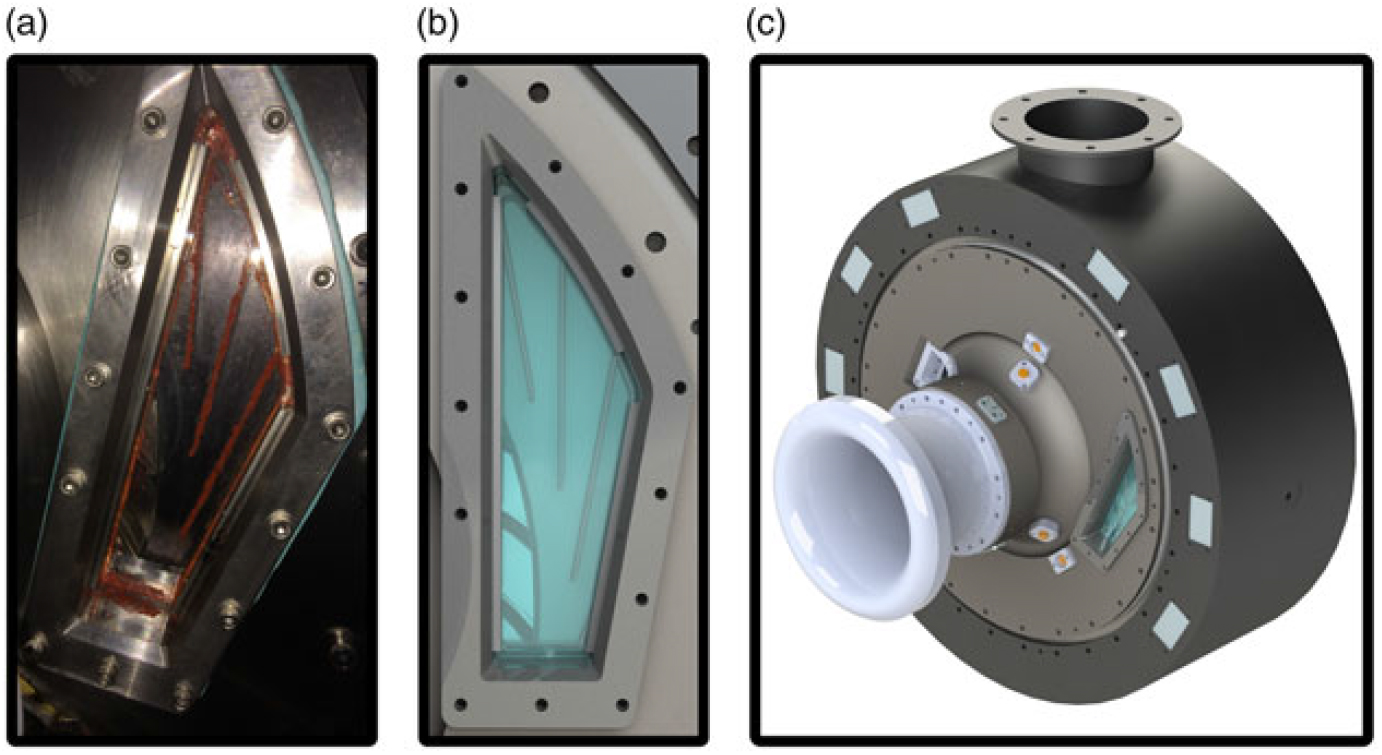
Figure 1. Photograph (a) and CAD rendering (b) of the diffuser access window and CAD rendering of the test stage (c).
A once-per-revolution (OPR) signal from the impeller is utilised to tag each velocity measurement with the instantaneous rotor angular position to allow ensemble averaging. This is critical for high-speed tests as the rotational frequency can be higher than the mean data rate of the LDV system, and ensemble averaging is necessary to resolve the blade-to-blade variations.
Careful design of the seeding apparatus and seed particles is critical to obtaining meaningful results. A TSI 9306 six-jet atomiser is used to generate an aerosol of Di-Ethyl-Hexyl-Sebacate. The seed is injected parallel to the flow upstream of the impeller inlet. An actuating mechanism is used to locally seed individual streamtubes. The injection point is adjusted until the data rate is maximised. This minimises the amount of overall seed to be injected – maximising test duration – while maintaining adequate seed levels in the MV.
The uncertainty analysis procedure given in Ref. Reference Orloff and Snyder18 applied to these data yields a typical uncertainty of less than ±1% in the streamwise and pitchwise velocities, ±2% in the spanwise velocity, and ±1° in flow angle. In regions of separated flow and adjacent to walls, where the signal-to-noise ratio (SNR) decreases, these values can nearly triple. The reduced resolution of the spanwise velocity occurs for two reasons; the requirement to measure this component at an angle of approximately 30° rather than directly and the lower output power of the 476.5nm band of an argon ion laser. The latter could be improved by a modification of the beam supply apparatus(Reference Boutier, Pagan and Soulevant19). The former is typically unavoidable in applications where optical access is difficult to obtain without significant and costly hardware modifications.
3.0 CONSIDERATIONS FOR TURBOMACHINERY
Multiple special considerations are required to yield meaningful results in the unique flow environment within turbomachinery. Sharp velocity gradients, high-frequency flow changes, large turbulence intensities, and small passages, among other aspects, impede the acquisition and quality of data.
3.1 Measurement volume size
Resolving the sharp velocity gradients within turbomachinery requires a small MV. The ellipsoidal MV is formed by the intersection of a pair of Gaussian beams at a point, as shown in Fig. 2. The three characteristic diameters of the MV, d x, d y, and d z, are expressed by:
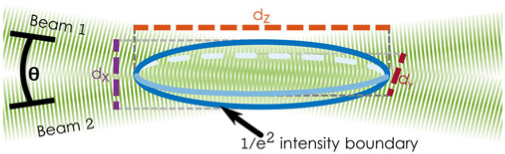
Figure 2. Measurement volume.
 $${d_x} = {{4\,\lambda \,f} \over {{\rm{\pi }}\,{d_w}\cos ({\rm{\theta }}/2)}}$$
 $${d_y} = {{4\,\lambda \,f} \over {{\rm{\pi }}\,{d_w}}}$$
 $${\rm{and}}\,{d_z} = {{4\,\lambda \,f} \over {{\rm{\pi }}\,{d_w}\sin ({\rm{\theta }}/2)}}$$
where λ is the wavelength of the beam, f is the focal length of the lens, d w is the initial diameter of the beam at the face of the focussing lens, and θ is the angle between the incident beams(Reference Albrecht, Borys, Damaschke and Tropea8). The number of interference fringes, N f , indicative of the quality of obtained Doppler signals, is expressed by:
 $${N_f} = {{8f} \over {{\rm{\pi }}\,{d_w}}}\tan \,({\rm{\theta }}/2)$$
To maintain the Doppler frequency within reasonable bandwidth limits, the angle θ is typically small(Reference Buchhave and Polyakov20). This results in the length of the MV in the beam direction being significantly longer than the other axes. This elongated axis often aligns with the spanwise direction in turbomachinery. For machines with small blade heights, the reduced spatial resolution poses an issue for experimentalists. Additionally, strong spanwise velocity gradients can create significant velocity gradients across the MV which impedes the resolution of turbulence quantities(Reference George and Lumley21).
These issues can be mitigated by operating in coincident mode or by utilising off-axis collection. Coincident mode, for multi-component systems, only accepts bursts which have produced a valid signal for each component being collected. This effectively reduces the MV to the overlap region of the ellipsoidal MV of each pair of beams. Off-axis collection reduces the MV to the overlap of the normal ellipsoidal MV with the receiver field of view(17). Assuming equal dimensions between the two overlapping regions and an angle between them of φ, an approximation of the new maximum dimension, d max, and the ratio to the original d z is expressed by:
 $${d_{\max }} = {{{d_x}} \over {\sin \,({\rm{\varphi }}/2)}}$$
 $${\rm{and}} = \left( {{{{d_{\max }}} \over {{d_z}}}} \right) = {{\tan \,({\rm{\theta }}/2)} \over {\sin \,({\rm{\varphi }}/2)}}$$
For a representative value of θ = 13.75°, this allows the maximum dimension of the MV to be reduced by half for an angular offset of φ = 28°. This significantly improves the spatial and turbulent-fluctuation resolution with only a small decrease in the data rate.
3.2 Reflection mitigation
Stray reflections from walls, windows, or other particles increase the noise floor of the photodetectors and impede data acquisition(Reference Albrecht, Borys, Damaschke and Tropea8). Passages for turbomachinery are typically narrow and composed of metallic walls and, consequently, are prone to significant reflections with the concomitant SNR reduction. In many cases, this prevents measurements close to walls as reflections from the primary beams saturate the MV.
The effect of reflections is reduced using special coatings or modifications to the flow passage boundaries. Anti-reflective coatings with high transmission rates in the range of wavelengths and incident angles utilised must be applied to both surfaces of windows used for optical access. This has the dual benefit of reducing stray reflections and increasing the laser power delivered to the MV. As an example, an uncoated fused silica window with a beam angle of 45° incidence can reflect approximately 10% of an incident beam at each interface. A specialised coating can reduce this to less than 0.5%(22). For solid boundaries, the incident light must often be absorbed (rather than transmitted) to reduce reflections. Stahlecker et al.(Reference Stahlecker, Casartelli and Gyarmathy23) replaced the hub surface with a specialised piece of absorption glass to absorb 87% of incident light, allowing measurements within 0.7mm of the endwall. Alternatively, absorbing black coatings may be applied to the metal surfaces. This approach requires fewer modifications to existing hardware; however, care must be taken to ensure that the absorbed energy can be dissipated by the coating without damage. A final consideration when choosing a coating material is its possible interaction with the seed particles. Certain coatings are oleophilic or hydrophilic and can increase the condensation rate of the seed, reducing testing time.
This reflection mitigation is critical in obtaining velocity data within the boundary layer or very close to solid surfaces where the stray reflections are strong and can easily oversaturate the signal. The other important considerations for obtaining useful data in the boundary layer are a small MV perpendicular to the solid surface being approached (for adequate spatial resolution within the boundary layer) and a precise knowledge of the MV location.
3.3 Seed particle size and injection
LDV systems for high-speed turbomachinery rely upon the accurate flow-following behaviour of seed particles artificially introduced into the stream. For a liquid or solid seed particle in a gaseous flow, the inertia of the particle acts as a low-pass filter in terms of responding to velocity fluctuations in the flow(Reference Albrecht, Borys, Damaschke and Tropea8). This cut-off frequency, f c, for a particle to follow the flow with an allowable slip (the relative difference between the particle and flow velocity), s, is given by:
 $${{\rm{f}}_c} = {1 \over {{{\rm{\tau }}_0}}}{1 \over {2{\rm{\pi }}}}\sqrt {{1 \over {{{(1 - s)}^2}}} - 1} $$
In Equation (8), τ0 is the characteristic timescale of the particle, defined as:
 $${{\rm{\tau }}_0} = \left( {{{{\rho _p}d_p^2} \over {18{{\rm{\mu }}_f}}}} \right)$$
where ρp, d p, and μf are the particle density, particle diameter, and dynamic viscosity of the fluid, respectively. This shows that the frequency response of seed particles is inversely proportional to the diameter squared. However, Rayleigh scattering theory shows that the amplitude of the scattered signal decreases with the sixth power of diameter for small particles. Particles, therefore, must be generated with a narrow size distribution that is small enough to follow the highest frequency fluctuations expected in the flow and no smaller to yield the highest possible signal quality.
The particle size distribution can be designed by choosing the seed generation method, the substance, the solution concentration, and the parameters of the seeding device. The distribution of seed particle diameters used in this study is shown in Fig. 3 along with the corresponding cut-off frequency for 1% and 5% slip. For this seed schema, 95% of the particles are expected to follow fluctuations of 25kHz at 1% slip or 57kHz with 5% slip. The blade-passing frequency is 11.25kHz, and these particles are expected to adequately follow the flow. This highlights the need for extremely small particles to resolve the high-frequency oscillations that characterise turbomachinery flows.

Figure 3. Particle size distribution.
The introduction of seed particles into the flow must also be considered. As mentioned previously, localised seeding offers a significant advantage over global seeding in terms of achievable test time. An actuated mechanism was used to introduce seed particles into a single 13mm diameter streamtube in the plenum, 200mm upstream of the inlet plane of the impeller. This injection point was shifted until the data rate was maximised and the optimum injection point remained relatively constant through the diffuser test campaign. Test times as long as three hours were achieved before condensation on the window interfered with data acquisition.
Seed must be introduced far enough upstream to allow the particles to accelerate to the local flow velocity. The relaxation time for particles much denser than the flow medium simply becomes the characteristic timescale of the particle, τ0. A particle injected at zero velocity will accelerate to within 1% of the flow velocity within a time of 6.9τ0 (Reference Albrecht, Borys, Damaschke and Tropea8). Streamlines in a steady CFD simulation were utilised to show a time of 37τ0 from injection to the forward-most measurement location, indicating sufficient particle adjustment.
Finally, the desired concentration of seed particles must be determined. The intuitive goal is maximum possible seed density to maximise the data acquisition rate. However, saturation of seed can interfere with data acquisition. Multiple particles being present in the MV violates the typical ‘single realisation’ assumption(Reference Albrecht, Borys, Damaschke and Tropea8). The Poisson probability distribution discussed in Section 1.3 can be used to show that the probability of this occurring for this study is only 0.1% (N ≈ 51 per mm3 and V ≈ 0.000897mm3). Particle coagulation must also be considered, especially for closed-loop test facilities where the long residence of particles allows significant coagulation at relatively low seed concentrations (see panel 10.18 in Ref. Reference Durst, Melling and Whitelaw5 and Chapter 13 in Ref. Reference Seinfeld and Pandis24). Similarly, high particle concentrations can violate the particle independence assumption underlying the determination of spectral response. On a general basis, an average particle separation of at least 1,000 diameters is considered sufficient(Reference Albrecht, Borys, Damaschke and Tropea8). This separation was approximately 1,300 diameters for this study. These analyses have been conducted using the seed concentration of the output of the seed generator. Some dilution will occur between the seeded streamtube and the surrounding flow; however, the worst case (in terms of a saturation of seed) corresponds to no dilution occurring. In the extreme, seed particles can act to damp turbulent fluctuations(Reference Hetsroni and Sokolov25) and violate the single phase flow assumption regarding the field being studied. However, the SNR, in most applications, will deteriorate prohibitively before these considerations become significant.
3.4 Traverse alignment and zeroing
Errors are introduced into the measurements if the traverse coordinate system is not precisely aligned with the axes of the test apparatus. Misalignment of the axes causes errors in applying the vector transformation from the LDV skew coordinate system to the laboratory Cartesian system. Additionally, measurements away from the origin will be geometrically shifted from their intended location proportionally to the degree of misalignment and the distance from the origin. The same issue arises for an improper zeroing of the traverse coordinate system to the true origin of the machine. In particular, a precise knowledge of the MV location relative to the lab reference frame is critical for boundary layer investigations. Even a small discrepancy in the interrogation location can cause serious errors in interpreting the boundary layer velocity profile and other quantities due to the sharp flow gradients present(Reference Boutier26).
A tool was designed to allow precise alignment of the traverse and the test apparatus quickly and easily, Fig. 4. This tool consists of a tight-tolerance machined surface to closely match the contour of the diffuser vane leading edge. Three 0.100mm diameter holes – labelled ‘Tool Zero Point’ and two forming the ‘Vertical Axis Reference’ in Fig. 4 – were micro-machined through the piece, and their orientation to each other and the location of the vane leading edge was inspected after machining.
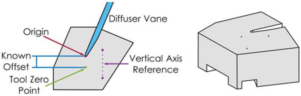
Figure 4. Traverse alignment tool.
After beam alignment, the MV was moved to the top of the vertical axis–reference pair of holes. The traverse system was translated vertically, and the alignment was adjusted until the two vertical axis–reference holes aligned with the vertical axis of the traverse. A similar process was used between the vertical axis–reference holes and the tool zero point to verify the horizontal axis alignment. The orthogonality of the traverse system itself was relied upon to verify the alignment of the third axis. The zero was established by passing the six crossed beams through the tool zero point and applying the measured offset between the tool zero point and the system origin placed at the diffuser vane leading edge. The estimated uncertainties, with contributions from the inspection, the positioning, and the traverse itself, are reported in Table 1. The propagation of alignment uncertainty into the velocity measurement uncertainty depends upon the angle between the LDV probes, the MV properties, the local velocity gradient, and the turbulence of the flow. Additional details can be found in Refs. 18, 20.
Table 1 Estimated uncertainties for system alignment

4.0 DATA PROCESSING
Turbomachinery applications require special consideration in the processing of LDV data. Many of these steps are familiar to other experimental methods such as hot-wire or unsteady pressure measurements. Some, however, are unique to LDV and other methods with relatively low SNR.
4.1 Ensemble and mean passage averaging
The first step is in computing the ensemble average and a mean passage representation. This assumes that subsequent revolutions of the impeller can be considered identical replications of each other, and, for the mean passage, that all individual passages are identical. First, during acquisition, the OPR signal is acquired to indicate the beginning of each impeller revolution. During processing, each validated Doppler burst is labelled with the instantaneous angular position of the impeller, as indicated in Fig. 5, step A. This information is used to compose an ensemble-averaged revolution where each revolution of acquired data is overlaid as shown in step B. At this point, the data should be examined to verify that the individual passages look similar to each other before proceeding. The ensemble-averaged revolution can then be subdivided into individual passages using the known geometric locations of the blades relative to the full impeller wheel, as shown in step C. Finally, each passage can then be overlaid, essentially a second ensemble average, to form a single mean passage data set, as shown in step D.
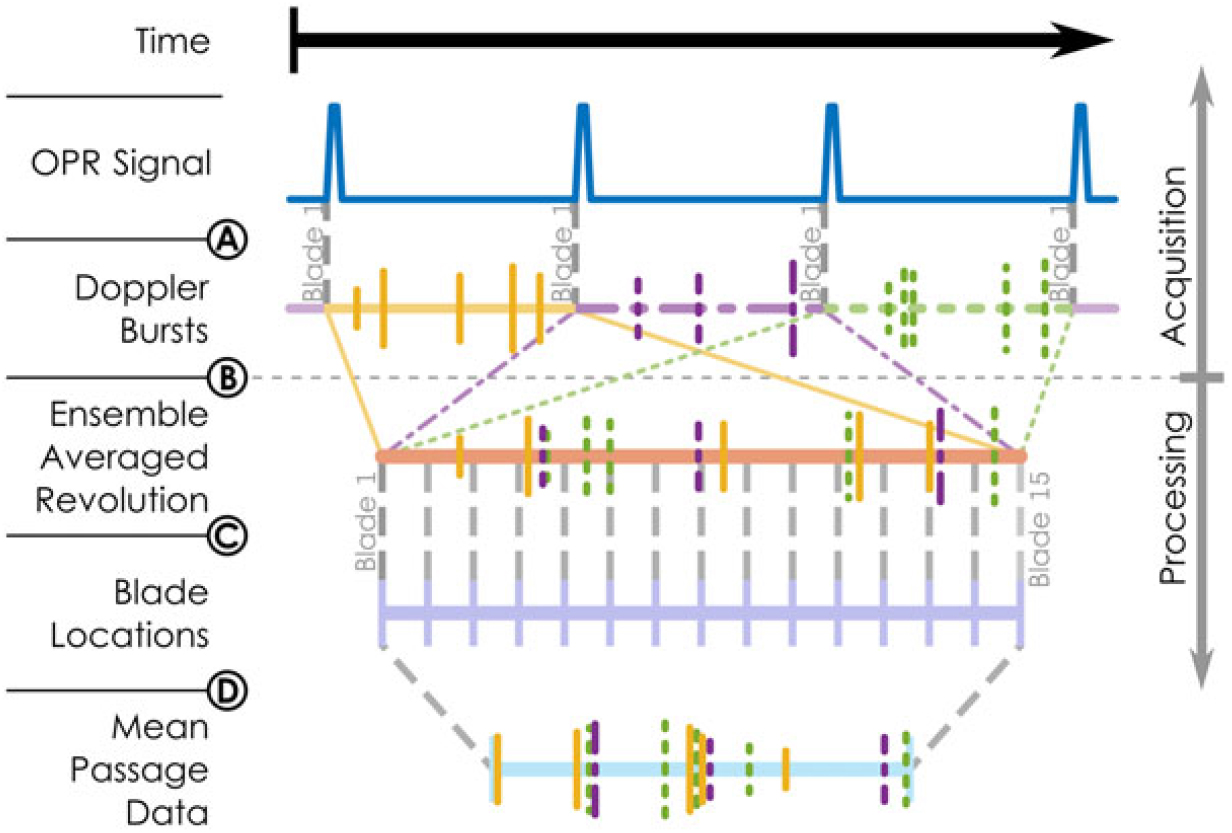
Figure 5. Averaging process.
4.2 Mixture-model-based noise isolation
Through the course of the experimental campaign, narrow bandwidth noise was observed in all three LDV channels. Two primary categories were observed. The first type was centred at zero velocity and occurred due to reflections through the MV. These reflections appear at a Doppler frequency equal to the Bragg cell shift frequency and result in a signal at zero velocity; an example is shown in Fig. 6(a). The second type was centred at a constant Doppler frequency of approximately 132MHz. The resulting velocity data were shifted between the three LDV channels due to the increase in fringe spacing with beam wavelength; examples are shown in Fig. 6(b) and (c). The source of this noise has not been isolated; however, the most likely sources are reflections from the rotating impeller or electromagnetic interference from another device. In many measurement locations, these noise sources could be removed using a band-pass filter during acquisition. However, since flow field velocities overlap with the spectral location of these two noise bands, a simple band-pass filter would remove true velocity measurements in some locations. For these cases, a post-processing method had to be developed to isolate and remove the erroneous measurements.

Figure 6. Examples of observed noise.
Manual identification and removal of the noise is a simple process. The noise bands were often dramatic, as evident in Fig. 6, and could easily be marked as invalid at the beginning of post-processing. However, the initial test campaign consisted of 794 individual measurement locations, each of which was subdivided into 24 time steps per blade passage and had three velocity channels. This resulted in 57,168 individual histograms requiring manual verification for the presence of noise. Since this is not a viable way to handle the large amount of data, an automated method is required.
The inspiration for this approach arose from a sabermetrics example using statistical mixture modelling to separate data drawn from two populations without knowing which sample belonged to which population(Reference Robinson27). This method uses an ‘expectation-maximisation’ iterative technique to separate each individual histogram of data into two groups. The continuous beta distribution was used since it is described by only two parameters yet still allows for skew which may be present in the data.
4.2.1 Expectation-maximisation algorithm
The first step in this approach is to initially divide the data into two groups. This is done in two ways. If a distinct mode is detected at one of the two expected noise centres, then the band of data surrounding that mode is placed in one group and the remaining data in the second. If this is not the case, then samples are assigned to a group randomly. A maximum-likelihood method is then used to fit a beta distribution to each of the two groups in the ‘maximisation’ step. When the initial groups are assigned randomly, these two distributions are nearly identical. However, there will always be a slight difference in the proportion of noisy data, if any, in each group. This means that noise-induced samples are marginally more likely to be in one of the groups rather than the other; the mixture modelling method exploits this slight difference to divide the data. In the case where noise is detected using a simple mode-based criterion, the two beta distributions will already be significantly different. Fig. 7 graphically depicts the entire mixture modelling procedure.
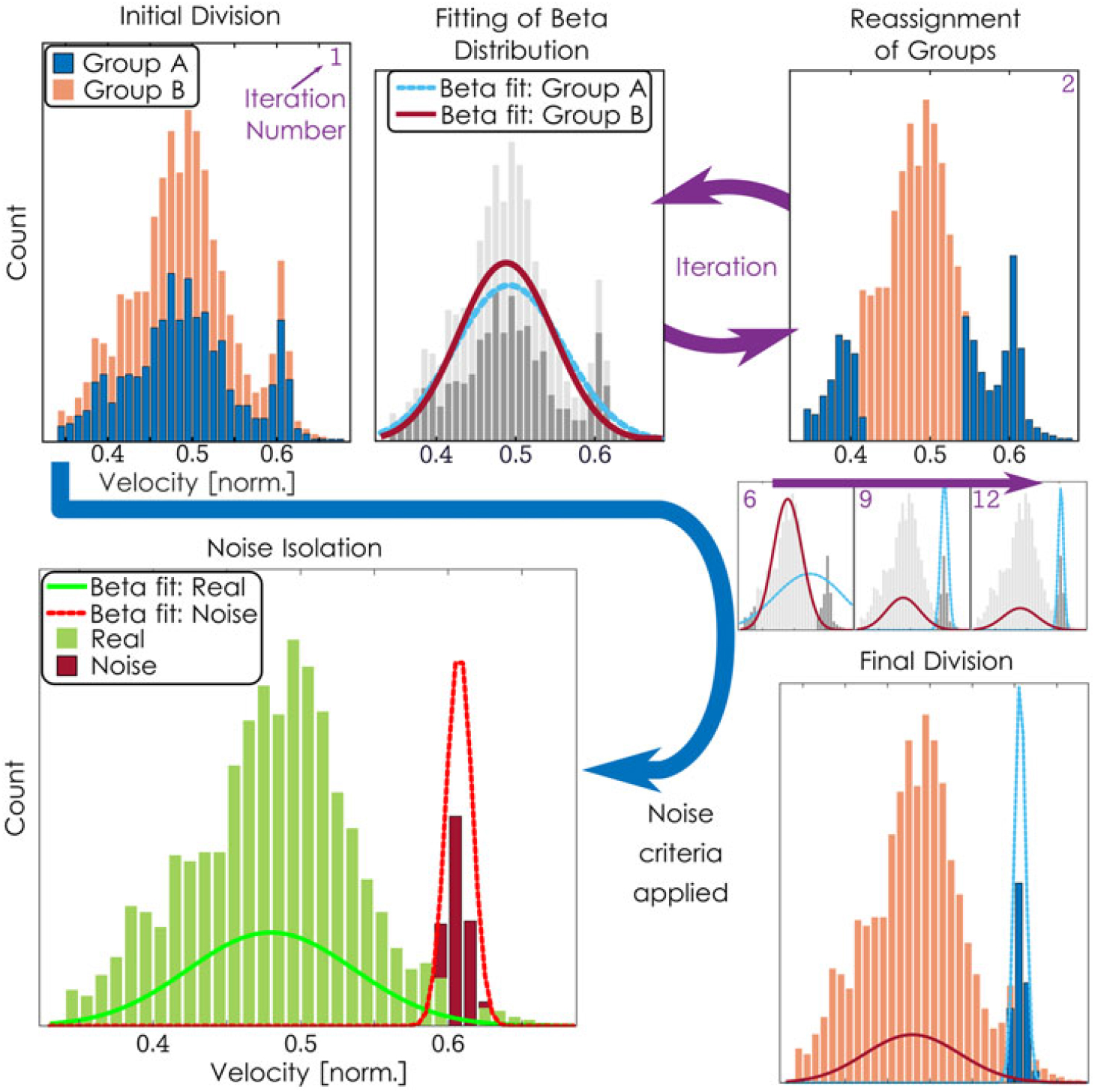
Figure 7. Mixture modelling process.
Using these distributions, two probabilities are computed for each of the original data points. The first probability is the value of the probability density function that was fit to group A multiplied by group A’s prior probability. The prior probability is a term from Bayesian statistics that, in this case, is simply the number of data points that were in group A on the previous iteration divided by the total number of data points. The second probability is the analogous value computed for group B. These two probabilities computed for each data point are then compared. If the probability corresponding to group A is greater, then the data point is placed into group A for the next iteration; otherwise, it is placed into group B. This forms the final portion of the ‘expectation’ step of the procedure, placing each data point into the more likely group.
This process – fitting beta distributions to each group and then reassigning groups based on those distributions – continues, iteratively, until the group assignments remain constant between iterations. In many cases, when no noise is present in the data, the result is that all data points are placed into a single group and the method accurately detects that no noise was present in the original data.
4.2.2 Noise determination
In cases where the converged solution contained two groups, the final step is to enact some criterion to determine which values can be discarded with high confidence. First, the group (either group A or group B) that contains the suspect data points must be determined. Comparing the mean of each group to the known noise centres and comparing the number of data points in each of the final groups allowed the group containing suspect data to be determined. Then, the probability that each data point belonged to the noise distribution was computed applying Bayes’ theorem:
 $$P({U_i} \in \,noise) = {{{\rm{Beta}}({U_i};{{\rm{\alpha }}_{{\rm{noise}}}},\,{{\rm{\beta }}_{{\rm{noise}}}})} \over {{\rm{Beta}}({U_i};\,{{\rm{\alpha }}_{{\rm{noise}}}}{\rm{,}}\,{{\rm{\beta }}_{{\rm{noise}}}}) + Beta\,({U_i};\,{{\rm{\alpha }}_{{\rm{real}}}}{\rm{,}}\,{{\rm{\beta }}_{{\rm{real}}}})}}$$
where U i represents an individual velocity sample and ‘Beta(U i; α, β)’ refers to the probability density function of the beta distribution evaluated at U i with the parameters α and β. These parameters are the values that were fit to each group of the converged iterative process. If this probability is greater than a cut-off value (0.95 in this study), then the data point was labelled ‘noise’.
4.2.3 Method validation checks
Any newly developed post-processing methodology must be validated to ensure it is functioning as expected. Several such checks were conducted and built into the post-processing Matlab code. Images of the final histograms showing the data labelled as ‘noise’ were selectively saved for visual inspection. Every case that met one (or more) of the following three criteria were written out: if more than 5% of the original data was labelled as noise, if the mean of the ‘noise’ differed from the anticipated noise centres, or if the noise removal shifted the data mean by more than 3 m/s. These ‘flagged’ outputs allowed the user to verify that any shifts caused by the algorithm were correct by visually verifying that the removed data were, in fact, noise. In the first implementation, a random 1% of the final histograms was also outputted to check the proper behaviour of the algorithm in cases where no significant data were filtered as noise. Fig. 8 shows several example outputs, and the overall validation results are summarised in Table 2.
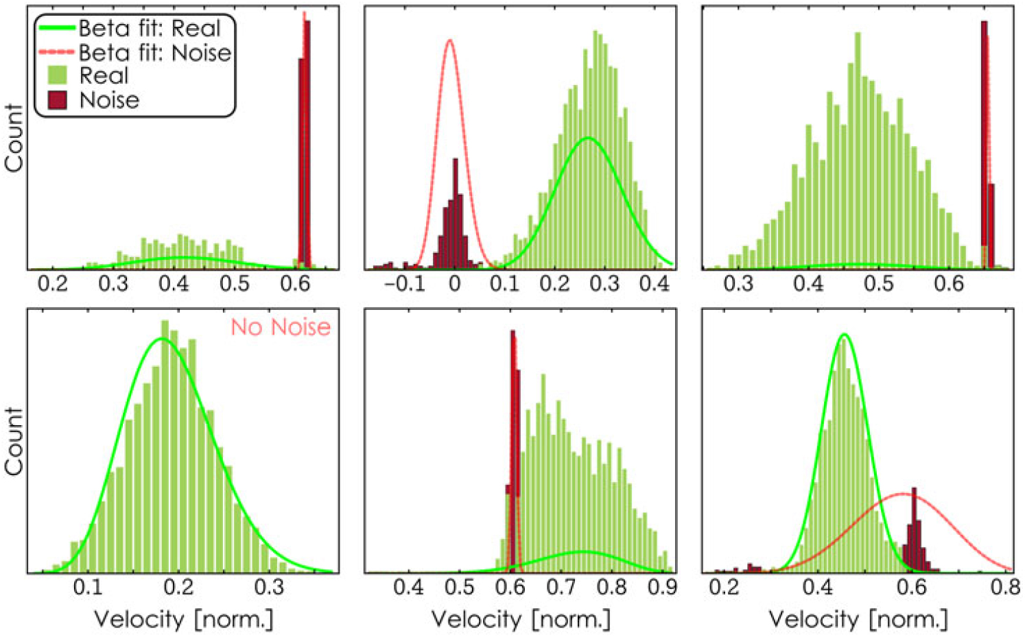
Figure 8. Noise removal example results.
Table 2 Process validation results

The percentage of ‘flagged’ results that were incorrect represents the proportion where noise was labelled incorrectly by the algorithm. The percentage of randomly outputted results that were incorrect represents the ‘false-negative’ (or type II error) rate where no noise was detected when noise was present. Even in this single false-negative case, the mean of the properly filtered result was shifted by less than 1.5%. Additionally, a 99% confidence interval on the true proportion of false negatives yields an upper bound of 1.3%. These results show that the method correctly identifies results that need further study. A similar confidence interval on the proportion that was incorrectly filtered yields an upper bound of 2.7% incorrect. This supports the high accuracy of the method.
The primary goals of the post-processing method have been achieved: it correctly removes data, it rarely misses noise that is present, and it greatly reduces the number of manual inspections required (from 57,168 to 2,394, a reduction of 95%).
5.0 EXAMPLE RESULTS
The detailed flow field resulting from this experimental study will be presented in a future paper; however, the following figures present a small sample of the obtained data. Fig. 9 depicts the axial (from shroud towards hub) velocity measured at 85% span through the vaneless space and diffuser inlet region at a single relative impeller-diffuser orientation. The raw, unfiltered results are on the left while the results after the mixture-model-based filtering algorithm is applied are on the right. The differences between the two datasets are most pronounced closest to the impeller tip as the noise source at 132MHz was more significant closer to the impeller. This supports the hypothesis that the noise arose from reflections off of the rotating impeller blades. As evident in the figure, the filtering process allowed the different axial velocities in the impeller jet and wake regions to be more coherent. The jet (closer to the pressure or leading side of the blade) has a band of strong shroud-to-hub secondary flow (yellow) while the wake has a band of strong hub-to-shroud secondary flow (blue).
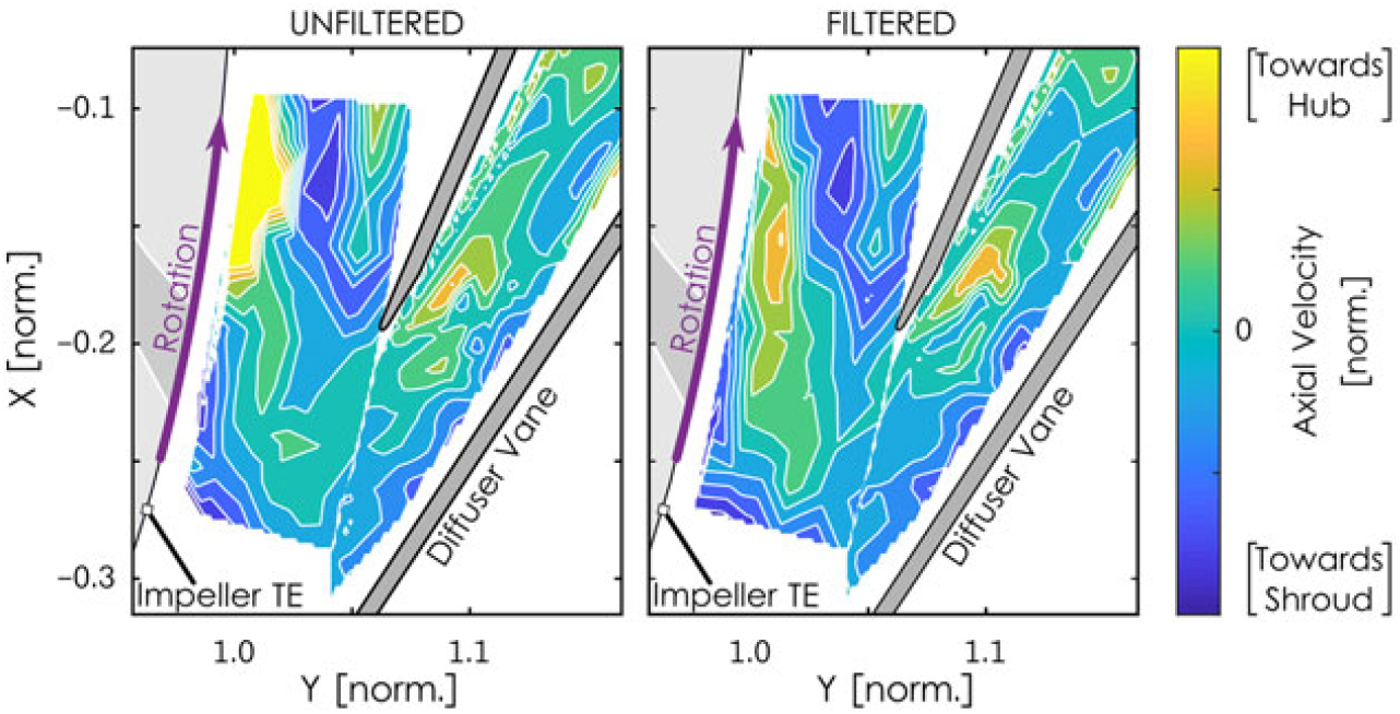
Figure 9. Instantaneous axial velocity contours at 85% span.
The noise was most prevalent within the third component of the LDV system (utilising the 476.5nm wavelength) which was used primarily to determine the spanwise (axial) velocity. Therefore, the filtering algorithm had the largest benefits in the resolution of the secondary flow characteristics in the spanwise velocity component. The unfiltered and filtered results in the other components showed fewer significant differences. An example of these results is given in Fig. 10 depicting the unsteady flow angle at a radius ratio of 1.025, relative to the impeller tip radius. The projected location of the downstream diffuser vane is illustrated as well as the instantaneous location of the full and splitter blades. On this stage, the splitter blades begin at 34% of the meridional impeller passage. Impeller rotation is from left to right in the figure. The flow angle is measured relative to a reference value – positive values indicate more tangential flow trajectory while negative values indicate more radial flow. Each row corresponds to a separate time step (TS) equally spaced through one full blade passing event, and the unfiltered and filtered data are in the left and right columns, respectively.
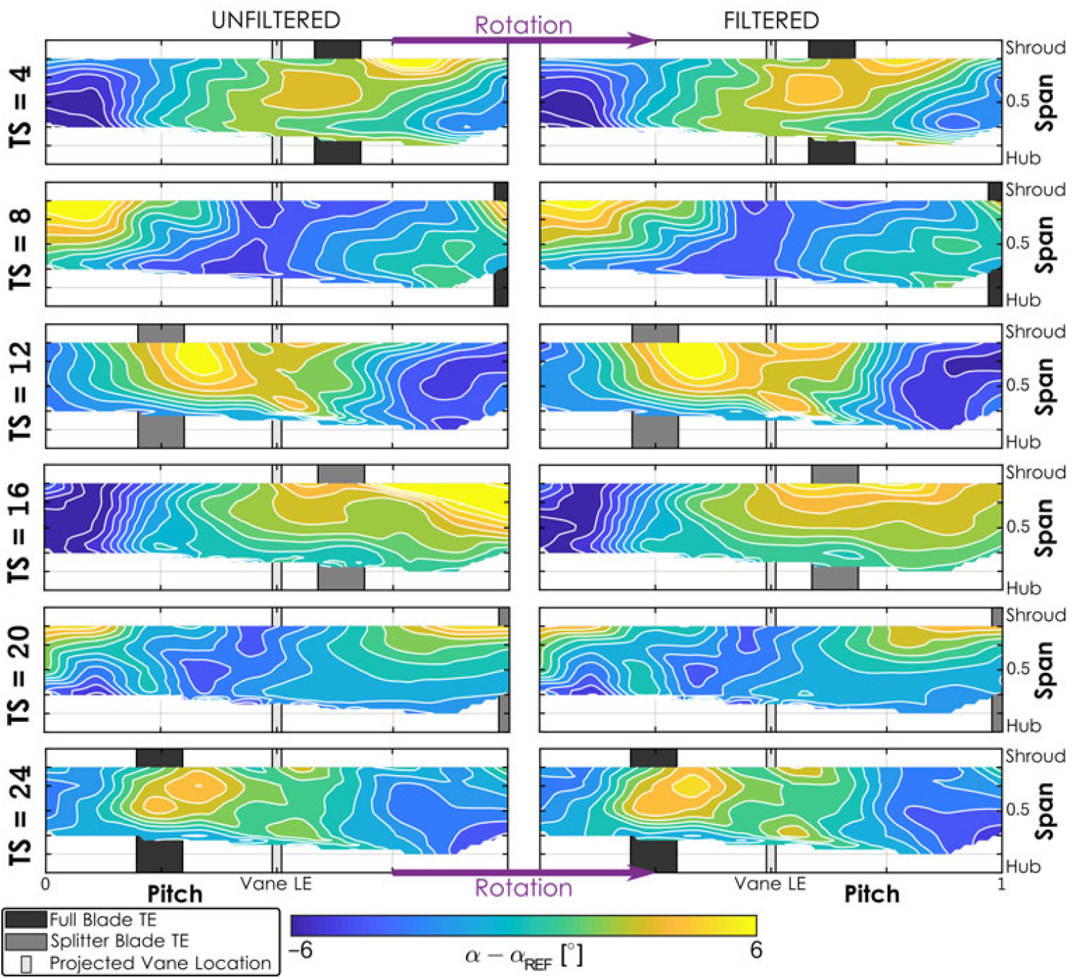
Figure 10. Unsteady flow angle contour at a radius ratio of 1.025.
Although the differences are less dramatic than in the axial velocity data (Fig. 9), the benefits of the filtering algorithm are still evident. For example, the severity of the tangential flow preceding the full blade at TS = 4 (first row) is reduced. Additionally, the contour of the flow angle preceding the splitter blade at TS = 16 (fourth row) is significantly clarified by the algorithm. These two example results are presented only to illustrate the benefits gained through the noise-filtering algorithm.
As with any new processing technique, caution and the careful judgement of the user must be utilised. Automated techniques can offer tremendous benefits; however, they can also have tremendous consequences if not applied carefully and with checks in place. This model, in particular, has the advantage of having no ‘tuning’ coefficients that need to be tailored to each new application. However, the user must carefully evaluate the effects the filtering process has had on the data and ensure that those effects, and any dependent observations or conclusions, are not artificially introduced by the method.
6.0 CONCLUSIONS
Steps required for proper acquisition and processing of laser Doppler velocimetry data for turbomachinery research applications were reviewed. Various common difficulties that arise in these applications were presented and potential solutions discussed. The specific challenges of turbomachinery applications – narrow internal passages, sharp velocity gradients, large turbulence intensities, and high-frequency fluctuations, among others – often result in low overall SNR and narrowband noise sources that cannot be removed by simple band-pass filters. Off-axis collection allows spatial resolution to be improved without sacrificing velocity measurement accuracy. The narrow passages of turbomachinery also require coatings be used to mitigate reflections in order to obtain adequate SNR. Aspects of properly engineered seed schema – both in terms of particle size and localised injection – were also presented along with a method for precise traverse system alignment. These techniques have been applied to successfully obtain three-component, unsteady velocity data from a high-speed centrifugal compressor for aeroengine application for the first time (to the authors’ knowledge). A newly developed mixture-model-based statistical method for narrowband noise isolation was described and validated. The method demonstrated successful rejection of noise with high accuracy, a low failure rate, and a significant reduction in manual inspection required. This newly developed method elucidated flow features that were not distinguishable prior to the noise removal. Further work on the applicability of this processing technique to other datasets is required.
ACKNOWLEDGEMENTS
The authors would like to thank Rolls-Royce Corporation for its funding and permission to publish this work. They would also like to acknowledge the team, Ruben Adkins-Rieck and Matt Meier; the Purdue Compressor Lab staff, John Fabian and Grant Malicoat; and the Zucrow staff, Rob McGuire and Toby Lamb, among others for their extensive support in myriad capacities throughout this project. Finally, the extensive technical advice and guidance of Cliff Weissman from Dantec Dynamics was crucial to the success of this study.


 Open access