


1. Introduction
In the study of boundary layer transition, an idealistic approach is to use an infinitely thin flat plate. This type of approach has been adopted in many former direct numerical simulation (DNS) and large eddy simulation studies, on free-stream turbulence (FST) induced boundary layer transition, by starting the simulation at some downstream distance from the origin of the boundary layer (Rai & Moin Reference Rai and Moin1993; Voke & Yang Reference Voke and Yang1995; Jacobs & Durbin Reference Jacobs and Durbin2001; Brandt, Schlatter & Henningson Reference Brandt, Schlatter and Henningson2004; Zaki & Durbin Reference Zaki and Durbin2006). The reason is partly attributed to the intricacy of treating complex geometries, such as a leading edge (LE), in many computational codes. Partly due to a dramatic increase in computational cost, and partly due to lack of knowledge regarding the significance of the LE in FST induced transition. In reality, there is always an inevitable LE with an associated local pressure gradient given by the profile shape and its stagnation line. The stagnation line is the extended stagnation point in the spanwise direction of the LE; see figure 1(a) for an illustration. The LE region, with its thin boundary layer, is believed to be a critical location for boundary layer receptivity in the transition process. Receptivity, as first coined by Morkovin (Reference Morkovin1969), is a stage in the transition process where external disturbances, such as acoustic, vorticity or FST disturbances, first enter the boundary layer and where rapid adjustments in the boundary layer flow take place. A receptivity coefficient links the disturbances penetrating the boundary layer to the response of the boundary layer. The inherent local pressure gradient imposed in this region of curvature and its effect on transition is not fully understood and is here given specific attention since this region provides the initial conditions for the successive boundary layer development (Reshotko Reference Reshotko1984).

Figure 1. (a) Sketch of a LE. The stagnation line is the extended stagnation point ( $x_{{s}}$) in the spanwise direction (i.e. $z$-direction) at the LE. (b) Schematic of the experimental set-up 1 (dimensions are in mm). The focused region in the circle highlights an electret condenser microphone embedded inside a cavity under a pinhole orifice.
Leading-edge pressure gradients and different types of LE geometries have been studied extensively in the past but mainly with focus on low background disturbance levels and are hence not reviewed, but referenced here for the interested reader; see e.g. Kendall (Reference Kendall1991), Klingmann et al. (Reference Klingmann, Boiko, Westin, Kozlov and Alfredsson1993), Saric, Wei & Rasmussen (Reference Saric, Wei and Rasmussen1995), Watmuff (Reference Watmuff1997), Wanderley & Corke (Reference Wanderley and Corke2001), Li & Gaster (Reference Li and Gaster2006). In general, there are two important considerations when selecting the LE for a fundamental study. (1) The curvature at the juncture between the LE and the extending flat plate should be continuous, i.e. zero, which can be ensured by using super-elliptic LEs. A discontinuous curvature provides a source of receptivity, which will influence the stability of the boundary layer. (2) A thicker LE will give rise to a stronger adverse LE pressure gradient (i.e. a larger suction peak) which in turn will affect the boundary layer stability due to a potential slightly inflectional velocity profile.
In the FST induced transition study by Nagarajan, Lele & Ferziger (Reference Nagarajan, Lele and Ferziger2006) using a mixed direct and large eddy simulation technique, a super-elliptic LE was used with two different aspect ratios ( $AR$) and different FST conditions. The LE pressure gradients show clear suction peaks but are modestly changed between $AR = 10$ and $AR = 6$. There are two direct LE comparisons with two different FST conditions. Both at relatively large turbulence intensities ( $Tu$) 3.5 % and 4.5 % with a 50 % larger integral lengths scale for the higher $Tu$ level. In both comparisons (their cases A with E and C with D) the onset of transition (minimum $C_f$ value) is changed by about 10 %, moving upstream with a blunter LE.
Ovchinnikov, Choudhari & Piomelli (Reference Ovchinnikov, Choudhari and Piomelli2008) carried out DNS with a super-elliptic LE geometry, with two computational configurations and boundary conditions, one simulating the half-plane with a symmetry condition upstream of the LE and the other simulating the full domain around the LE. Their observations suggest that the LE couples velocity fluctuations normal to the plate axis at the LE to initial levels of the streamwise Reynolds stress in the developing boundary layer. They conclude that the symmetry condition attenuates this mechanism leading to reduced streamwise velocity fluctuations in the downstream boundary layer. Furthermore, they report their expectation that the observed receptivity mechanism will be sensitive to the geometry of the LE, for example, through the effect of the LE curvature. However, their study did not include LE pressure gradient variations and, hence, the effect can not be assessed from their results. In a later DNS study by Zaki (Reference Zaki2013), the shear-sheltering phenomenon in transitional boundary layers was investigated simulating a complete elliptic LE in combination with a flat plate. They demonstrate that the type of secondary instability which leads to turbulent spots can be dependent on the pressure gradient history and LE geometry itself. However, the effect of the LE pressure gradient was not addressed per se. From these works it is, however, clear that to accurately capture the receptivity process a full LE simulation is required.
For an accurate prediction of the onset of boundary layer transition caused by FST, the initial FST condition prevailing at the LE, namely the integral length scale ( $\varLambda _x$), the turbulence intensity ( $Tu$) and the free-stream speed ( $U_\infty$) are of prime importance (Fransson & Shahinfar Reference Fransson and Shahinfar2020). It is an arduous task and computationally very expensive to perform a parameter variation study particularly changing both the initial FST condition and the LE pressure gradient, which are two essential factors that determine the location of transition onset. Heretofore, there are no quantitative studies reported either through numerical simulations or experiments on the influence of the leading-edge pressure gradient region in boundary layers subject to FST. The present experimental investigation is aimed at quantifying the influence of the LE pressure gradient for different FST conditions on the transition process. Special attention has been given to the adjustment of different conditions used in this study. Furthermore, in the study by Fransson & Shahinfar (Reference Fransson and Shahinfar2020) a scale-matching model was introduced to include the effect of $\varLambda _x$ in the prediction model but their hypothesis that, for each $Tu$, there exists an optimal $\varLambda _x /\delta _{{tr}}$ that promotes transition to a lowest possible $Re_{{tr}}$ could not explicitly be validated since the FST conditions were randomly generated. Here, $\delta _{{tr}}$ is the boundary layer scale at transition. The prediction model seemed to physically capture the influence of $\varLambda _x$ on $Re_{{tr}}$ correctly, which provided an indirect confirmation of the hypothesis. However, in the present investigation we are able to test the hypothesis directly by generating different FST conditions in a more sophisticated way, i.e. we make sure to keep $Tu$ constant as we vary $\varLambda _x$. In addition, in this analysis the variation of the LE pressure gradient is included which provides important results.
This paper begins with an overview of the experimental set-ups accompanied by measurement techniques and quantification of pressure distributions in § 2. In this section § 2.4 we give a brief description of the quantitative estimation of intermittency based on wall-pressure time signals using Hilbert transform and adaptive threshold algorithms. The measurement results from a set of careful, multi-faceted experiments conducted using hot-wire probes, electret microphones and a time-resolved pressure transducer are discussed in § 3. Here, we also show the test result of the scale-matching hypothesis by Fransson & Shahinfar (Reference Fransson and Shahinfar2020). Lastly, in § 4 our main conclusions are drawn and summarised.
2. Experimental set-ups
2.1. Wind tunnel facility
The experimental campaign was performed in the minimum turbulence level (MTL) wind tunnel at KTH Royal Institute of Technology in Stockholm. The MTL is a closed-loop tunnel with a 7 m long test section and a cross-sectional area of  $1.2 \times 0.8\ \mathrm {m}^2$. The DC axial fan (85 kW) can generate a maximum speed of 69 m s $^{-1}$ in an empty test section. The velocity fluctuation level in the streamwise direction ( $u_{{rms}}$) is less than 0.025 % of the free-stream velocity ( $U_\infty$) at the nominal speed of $U_\infty =25$ m s $^{-1}$. A constant temperature within $\pm 0.05\,^{\circ }$C inside the test section can be achieved by means of a heat exchanger networked with an inbuilt PID controller. The total pressure variation inside the test section is less than $\pm$0.06 % (cf. Lindgren & Johansson (Reference Lindgren and Johansson2002) for more details).
Two different experimental set-ups with different flat plates, including different LEs, were used in this investigation to ensure set-up independency and result repeatability. In the following these are referred to as set-up 1 and set-up 2. Set-up 1 consists of a 4500 mm long flat plate (as shown in figure 1b) with a 260 mm long asymmetric LE and a 1600 mm trailing edge flap. The design and validation of the LE are reported in Fransson (Reference Fransson2004) and has been used successfully in several past investigations (cf. e.g. Fransson & Alfredsson Reference Fransson and Alfredsson2003; Yoshioka, Fransson & Alfredsson Reference Yoshioka, Fransson and Alfredsson2004; Fransson Reference Fransson2010). Set-up 2 consists of a 4200 mm long flat plate with a 160 mm long asymmetric LE and a 450 mm long trailing edge flap. This LE was first reported in Klingmann et al. (Reference Klingmann, Boiko, Westin, Kozlov and Alfredsson1993) and has also been used in many successful investigations (cf. e.g. Matsubara & Alfredsson Reference Matsubara and Alfredsson2001; Fransson, Matsubara & Alfredsson Reference Fransson, Matsubara and Alfredsson2005; Fransson & Shahinfar Reference Fransson and Shahinfar2020). Cartesian coordinates are used with ( $x,y,z$) corresponding to the streamwise, wall-normal and spanwise directions, respectively. The base flow on the flat plate was adjusted to a close to a zero-pressure gradient condition by means of the compliant ceiling of the test section. The trailing edge flap is used to fine-tune and adjust the stagnation line (see figure 1a) at the LE and since the flap lengths differ in set-ups 1 and 2, the reported trailing edge flap angles ( $\phi$) are not comparable in set-ups 1 and 2, instead the full LE pressure distribution has to be compared between the set-ups.
The plate in set-up 1 is new and is equipped with a total of 56 static-pressure taps out of which 16 are located on the LE itself, which allow documentation of the streamwise pressure distribution. In addition, a total of 100 microphones are embedded inside this plate in the streamwise direction to facilitate transition location measurements. Set-up 2 on the other hand does not have the above features, i.e. to measure static or fluctuating pressures.
To generate different FST conditions, characterized by the turbulence intensity ( $Tu=u_{{rms}}/U_\infty$) and the integral length scale ( $\varLambda _{x}$) at the LE, similar grids and numbering to Fransson & Shahinfar (Reference Fransson and Shahinfar2020), were mounted upstream of the LE on a rail system to ease the change in relative distance between grid and LE ( $x_{{grid}}$). The grids are characterized by its bar diameter $d$ and mesh width $M$, giving its solidity ( $\sigma$) as $\sigma =(d/M)(2-d/M)$, which corresponds to the ratio between the blocked area of the grid and the total cross-sectional area.
2.2. Measurements and instrumentation
Numerous transition studies (e.g. Jonáš, Mazur & Uruba Reference Jonáš, Mazur and Uruba2000; Fransson et al. Reference Fransson, Matsubara and Alfredsson2005; Fransson & Shahinfar Reference Fransson and Shahinfar2020) employ hot-wire anemometry with signal analysis to compute the intermittency factor ( $\gamma$), which enables an accurate determination of the transition location. However, as an aid to speed up this type of examination, a new approach for transition detection based on electret microphones (3 mm in diameter) has been employed in set-up 1. The advantage with respect to hot wire is the absent traversing time. The microphones are mounted inside a cavity under a pinhole orifice (focused in figure 1b) of a diameter 0.4 mm, making the top surface hydrodynamically smooth. It is important to note that undesired attenuation of the turbulent flow patches can occur if the wavelengths of the fluctuations are in the order of and smaller than the pinhole diameter ( $d$). To prevent the attenuation of the high frequency fluctuations, the diameter $d$ is kept within $d\leq 0.4$ mm (Lueptow Reference Lueptow1995). In addition, the Helmholtz's resonance of the cavity in which the microphone is embedded should be avoided. To limit the redundancy of the resonance, the ratio of the length ( $l$) of the orifice to the diameter ( $d$) should be constrained to $l/d\geq 2$ (Shaw Reference Shaw1960; Tsuji et al. Reference Tsuji, Fransson, Alfredsson and Johansson2007). The microphone signals were individually amplified using pre-amplifier circuits prior to acquisition. Simultaneous sampling of the microphone signals using a 256-channel high-end data acquisition (DAQ) system, incorporating NI 9205 modules mounted in an NI cDAQ-9189 chassis, provided a full streamwise intermittency distribution within a sampling time of 60 s. In our measurements a sampling frequency of 5 kHz was used.
A 64-channel miniature pressure scanner, Scanivalve MPS4264 module, capable of simultaneous time-resolved pressure measurements was used to obtain the static-pressure distributions on the plate via the static-pressure taps.
Both for characterizing the FST and for boundary layer velocity measurements, in-house manufactured single-sensor hot-wire probes operating in constant temperature mode using a DANTEC dynamics anemometer system (Streamline 90N10 frame, with 90C10 modules) were utilized. The hot-wire data was collected using a 16-bit, NI PCI-6259 DAQ system at a sampling frequency of 10 kHz. The probes were calibrated in the free stream inside the tunnel against the dynamic pressure obtained from a Prandtl tube, through a differential manometer (Furness FCO560).
2.3. Pressure distribution quantification
The angle  $\phi$ of the trailing flap that is adjusted to impose different LE pressure distributions is a set-up dependent parameter, and, therefore, not suitable to use as a measure for the LE pressure gradient. Instead, a single value that directly quantifies the pressure distribution, throughout the LE region, is sought after. In an inviscid and incompressible flow, the pressure coefficient can be expressed as a function of the local free-stream speed as
 \begin{equation} C_p(x)=1- \left( \frac{U(x)}{U_\infty} \right)^2.\end{equation}
Now, by making the following ansatz of the external free-stream velocity variation,
 \begin{equation} U(x)=C_1 U_\infty(x-x_0)^m,\end{equation}
on (2.1) we obtain
 \begin{equation} C_p(x)=1-C(x-x_0)^{2m}.\end{equation}
Here,  $C_1$( $>0$) and $x_0$ in (2.2) correspond to a stretching parameter and a virtual origin, respectively. The term $C(>0)$ in (2.3) is a new constant and $m$ is the well established acceleration/deceleration parameter that appears in the Falkner–Skan equation, which is derived by applying the ansatz (2.2) on the two-dimensional boundary layer equations. One clear advantage with $m$ over other established non-dimensional pressure gradient parameters is that the former is a non-local parameter and, hence, can be used to describe the pressure distribution in the entire LE region. In addition, once $m$ is determined it can with ease be used to predict both the shape and the thickness of the boundary layer throughout this region since the solution to the Falkner–Skan equation is a similarity solution.
Expression (2.3) can be fitted to the measured  $C_p$ distributions around the LE by means of least squares to obtain the coefficients $C$,
$C$,  $x_0$ and $m$. Note that in reality, for a zero-pressure gradient flow, the LE pressure $C_p$ will go to zero at some prescribed downstream location (cf. (2.1)). However, (2.3) indicates that $C_p\to \pm ~\infty$ as $x\to ~\infty$, which means that the assumption of (2.2) is only meaningful in the LE region. Hence, the fitting is only performed until $x=200$ mm, from where the pressure gradient is close to zero.
Throughout this paper, only the curvature  $m$ will be considered as a representative of the $C_p$ distribution, the other two constants are merely to improve the fit. In all the cases without suction peak, the first point is disregarded in the fitting process and the monotonically decreasing distribution gives $m>0$ (figure 2a). For the cases with suction peak (only set-up 2), the fitting is started from the $C_p$ minimum, resulting in $m<0$ (figure 2c). It shows that the relation between $m$ and the flap angle $\phi$ is close to linear (figures 2b and 2d) for both cases with and without suction peak, supporting that this is an appropriate measure to represent the pressure distribution around the LE in a single parameter value.

Figure 2. A systematic curve-fitting approach utilized in this study to estimate the parameter  $m$ in both set-ups 1 (a,b) and 2 (c,d), respectively. The circular markers indicate the measurement data. The solid black lines in (a,c) indicate the individual fits used to estimate $m$, and in (b,d) illustrate that $m$ is directly proportional to $\phi$.
2.4. Intermittency factor
In transitional boundary layers the onset, development and end of transition can quantitatively be described by the intermittency factor ( $\gamma$). The intermittent nature of the transitional flow can be captured by surface pressure signals obtained from microphones and post-processed to accurately calculate the $\gamma$-value. In this study a pressure-based intermittency function is adapted, which is new in contrast to the conventional velocity-based intermittency functions.
A well-established practice for transition location determination is where  $\gamma$ reaches 0.5, which is midway through the transition zone with the $\gamma$-values of zero and unity corresponding to a fully laminar and fully turbulent flow, respectively. Decision making tools like the detector/criterion functions and the adaptive threshold en route the user to assess and outline the transition region (cf. figure 3). Frequently used detector functions formulated on first or second derivative of the time signal as well as frequently used threshold values based on dual-slope method (Kuan & Wang Reference Kuan and Wang1990), region of maximum curvature (Hedley & Keffer Reference Hedley and Keffer1974) or logarithmic fit of $\gamma$ (Fransson et al. Reference Fransson, Matsubara and Alfredsson2005; Fransson & Shahinfar Reference Fransson and Shahinfar2020) are mainly flow dependent. In order to enhance the sensitivity to turbulent signatures, the detector function $\mathcal {D}(t)$, here, is merely a high-pass filtered microphone signal $e(t)$ where the cutoff frequency $f_{{cut}}$ has an objective constraint based on the local viscous scale ( $\delta =\sqrt {x \nu /U_{\infty }}$ ), i.e. $f_{{cut}}=n \times (U_{\infty }/\delta$). If $n$ can be chosen as a constant, the method becomes user independent and, hence, relatively robust. Based on a visual inspection study of different signals for multiple grids and free-stream speeds, the factor $n$ could be locked to a constant value $n=0.07$ for the microphone signals.

Figure 3. Turbulent patch detection algorithm used in the signal conditioning process. (a) The microphone time signal e(t) is in volts. The detector function  $\mathcal {D}(t)$ and the criterion function $\mathcal {C}(t)$ are calculated using the Hilbert transform. The intermittent regions marked in red correspond to the indicator function $\mathcal {I}(t)$ determined with a cutoff value $\mathcal {C}^{th}$ (here $\gamma =0.37$). (b) Direct comparison of $\gamma$-distributions obtained from microphones and a traversed hot wire with grid G6. The effect of varying the speed $U_\infty$ is illustrated for $U_\infty =6,8$ and 10 m s $^{-1}$. Solid curves in black indicate a sigmoid fit to each individual $\gamma$-distribution. Big circular markers correspond to $\gamma =0.5$.
To opt for a criterion function  $\mathcal {C}(t)$ which relies on $\mathcal {D}(t)$ is the critical step in the conditioning process. Here, we adopt the Hilbert transform, which is used in numerous applications such as speech recognition in audio signals (Ortiz et al. Reference Ortiz, Villa, Salazar and Quintero2016), activity detection in muscle cells from an electromyogram (Cao, Tian & Wang Reference Cao, Tian and Wang2019) or an electrohysterograph (Borowska, Brzozowska & Oczeretko Reference Borowska, Brzozowska and Oczeretko2016) and in electrocardiogram signals (Jorge et al. Reference Jorge, García, Córdoba, Bila and Mizera-Pietraszko2017). With the Hilbert transform ( $\mathcal {H}$), it is possible to derive an analytical representation of a real-valued detector signal $\mathcal {D}(t)$. If $\mathcal {H}$ is a bounded linear operator given by the integral
 \begin{equation} \mathcal{H}(\mathcal{D}(t))=\frac{1}{{\rm \pi} }\int_{-\infty}^{+\infty} \frac{\mathcal{D}(\tau)}{t-\tau} \, {\rm d} \tau , \end{equation}
then, an analytic signal  $z(t)$ can be written as
 \begin{equation} z(t)=\mathcal{D}(t)+i\mathcal{H}(\mathcal{D}(t)). \end{equation}
The criterion function  $\mathcal {C}(t)$ was computed as the convolution of $\lvert z(t) \rvert$ over successive small ‘smoothing intervals’ based on the sampling frequency. A suitable choice of an adaptive threshold $\mathcal {C}^{th}$ based on the root-mean-square of $\mathcal {C}(t)$ enabled us to quantify the turbulent and laminar regions in terms of an indicator function $\mathcal {I}(t)$ according to
 \begin{equation} \mathcal{I}(t)=\begin{cases} 1 & \text{if } \mathcal{C}(t) \geq \mathcal{C}^{th}, \\ 0 & \text{if } \mathcal{C}(t) < \mathcal{C}^{th}. \end{cases} \end{equation}
From the indicator function  $\mathcal {I}(t)$, evaluated for a particular intermittent microphone signal, the intermittency $\gamma$ is calculated as the temporal mean of $\mathcal {I}(t)$ or as the integral of $\mathcal {I}(t)$ over time normalized with the total time $T$, as
 \begin{equation} \gamma=\frac{1}{N}\sum_{i} \mathcal{I}(t)\text{ or } \frac{1}{T}\int_{0}^{T}\mathcal{I}(t)\,\mathrm{d}t, \end{equation}
 respectively. An example of how the transition location  $x_{{tr}}$ is calculated from the intermittency distribution where $\gamma =0.5$ is demonstrated in figure 3(b). Here, a sigmoid function in the form of $\gamma (x)=1-\exp [-\mathcal {\alpha }(x-\mathcal {\beta })^{c}]$ is fitted to each individual intermittency distribution to obtain $x$-locations where $\gamma =0.5$ ( $\mathcal {\alpha },\mathcal {\beta },c$ are the curve-fitted coefficients). The chosen shape of the intermittency function is inspired by the early work by Narasimha (Reference Narasimha1957) and later by Johnson & Fashifar (Reference Johnson and Fashifar1994). A significant amount of experimentally determined intermittency distributions have shown that the shape of the intermittency distribution is close to universal; see e.g. Fransson et al. (Reference Fransson, Matsubara and Alfredsson2005), Fransson & Shahinfar (Reference Fransson and Shahinfar2020) where all together over 80 different FST cases are included (see figures 16 and 5 in the respective papers). Based on all this data we see that we obtain the best individual fit, and, hence, the most reliable prediction of $\gamma = \gamma (x)$ if we let $c$ be a parameter to be determined through the curve fit as adopted here. We simply note here that according to the theoretical work by Narasimha (Reference Narasimha1957) and Johnson & Fashifar (Reference Johnson and Fashifar1994) the value of $c$ is 2 and 3, respectively.
In figure 3(b) the microphone performance of obtaining a full intermittency distribution is validated against the more common procedure using a hot-wire probe around the wall-normal location of maximum  $u_{{rms}}$ inside the boundary layer. Since the turbulent spot sweeping the probe has a speed of about 80 % of $U_\infty$ at this wall-normal location independent of $x$, which is contrary to the wall-mounted microphone where the speed is zero, the $n$-factor in $f_{{cut}}$ turns out to be different for the hot-wire signal ( $n = 0.04$) but then gives similar $\gamma$-distributions with associated threshold values $\mathcal {C}^{th}$. For the hot-wire signals, a constant threshold value is used while, for the microphone signal, the threshold turns out to vary linearly with $U_\infty$. As shown in figure 3(b), the comparison is good between the two techniques.
3. Results
In the present experimental study we examine the influence of the LE pressure gradient on the laminar-turbulent transition in the otherwise zero-pressure gradient flow on the flat plate while keeping all other parameters constant. The pressure coefficient ( $C_p$) in set-up 1 and set-up 2 is calculated using the static pressure along with the plate and by traversing a hot-wire probe at the constant wall-normal location $y=50$ mm, respectively. Here $C_p$ is calculated using pressure or velocity as
 \begin{equation} C_p(x)= \frac{p(x)-p_{{\infty}}}{p_0-p_{{\infty}}}=1- \left( \frac{U(x)}{U_\infty} \right)^2 , \end{equation}
where  $p_0$ and $p_\infty$ (as well as $U_\infty$) are obtained from the reference Prandtl tube mounted in the free stream over the plate at $x = 570$ mm.
3.1. Base flow and initial FST conditions
In figure 4(a),  $C_p$ determined from both the static pressure and hot-wire velocity data are plotted for set-up 1. The corresponding $m$-values from the static pressure, hot-wire data are $1.81\times 10^{-2}$ and $1.43\times 10^{-2}$, respectively. Wall-normal mean velocity profiles, normalized using the displacement thickness ( $\delta _1$), are plotted for different $x$-locations and compared with the Blasius boundary layer solution (solid line) in figure 4(b).

Figure 4. Adjusted base flow on the flat plate at  $U_\infty =6$ m s $^{-1}$ for set-up 1. (a) The streamwise $C_p$ distribution on the flat plate obtained both from hot-wire data and static-pressure taps. (b) Scaled wall-normal profiles of mean velocity. Different markers indicate individual $x$-locations from $50$–
$50$– $3200$ mm and the solid line corresponds to the Blasius solution.
The FST conditions at the LE, i.e.  $\varLambda _{x}$ and $Tu$, are calculated from a velocity-time signal measured by a hot-wire probe in the free stream at the LE of the flat plate. The integral length scale is calculated by integrating the autocorrelation function ( $R_{uu}$) of the velocity signal using the first crossing of the abscissa as the truncated lag value ( $\tau ^{*}$) and converting it to a length scale using Taylor's hypothesis as
 \begin{equation} \varLambda_x=U_\infty\int_{0}^{\tau^*}R_{uu}(\tau)\,\mathrm{d}\tau. \end{equation}
All cases with different FST conditions at  $U_\infty =8$ m s $^{-1}$ are summarized in table 1. For all the measurements reported in this paper, the standard errors of the mean for $Tu$ and $\varLambda _{x}$ are 0.006 % and 0.065 mm, respectively.
Table 1. Turbulence generating grids and FST conditions at the LE. The grid numbers are the same as used in Fransson & Shahinfar (Reference Fransson and Shahinfar2020).

3.2. Transition measurements: set-up 1
Adjusting the pressure gradient over the plate is an iterative process between ceiling and trailing flap angle adjustments. To obtain a zero-pressure gradient boundary layer, one needs to compensate for the boundary layer growths on the plate, ceiling and side walls, which makes four boundary layers. This means that the cross-sectional area needs to grow with the same rate as four times the displacement thickness of these boundary layers. In the MTL wind tunnel this area increase is accomplished by adjusting the ceiling. The trailing edge flap angle is used to fine-tune the location of the stagnation line (cf. figure 1a) at the LE which primarily affects the LE pressure gradient region. In the present study our reference pressure gradient case corresponds to  $m=3.3\times 10^{-2}$ ( $\phi = 13.9^\circ$, which is the angle where the ceiling was adjusted). From this case, we then systematically change $\phi$ to vary the parameter $m$, without altering the pressure gradient downstream of 150 mm for the cases that were chosen to be included in the transition study. Leading edge pressure gradients corresponding to $m$-values in the range of $8.5\times 10^{-3}-9.5\times 10^{-2}$ are shown in figure 5(a). For increasing flap angle, the stagnation line will move downstream on the upper side of the LE, eventually causing the flow to separate which happens when the flow cannot move upstream from the stagnation line and around the LE to the lower side any longer. In order to ascertain the critical flap angle for which this separation occurs the microphone signals at the LE were carefully analysed. For the transition studies, we therefore only include data for $\phi < 16^\circ$ ( $m<7\times 10^{-2}$). For the data in figure 5(b), this means that the $m=9.5\times 10^{-2}$ case is omitted since the flow is affected by LE separation while the second largest flap angle is included.

Figure 5. (a) Mean  $C_p$ distributions obtained from surface pressure data on the LE for different $m$-values. The arrow indicates the direction of increasing $m$. (b) Transitional Reynolds number vs parameter $m$ at $Tu=2$ % for different $\varLambda _{x}= [7.1~({\mathrm {C}}1), 15.8~({\mathrm {C}}4),$ $21.3~({\mathrm {C}}5)]$ mm. The dashed line indicates the reference case $m=3.3\times 10^{-2}$ where the FST conditions are tuned. (c) Transitional Reynolds number vs $m$ at different $\varLambda _{x}$ and $Tu$. Data from set-up 1; see table 1 for the different FST conditions.
The FST conditions at the LE ( $x=0$), i.e. $\varLambda _{x}$ and $Tu$, were adjusted at $m=3.3\times 10^{-2}$ and demonstrated only minor deviations for different flap angles. Furthermore, the pressure distribution on the flat plate is unaffected by the presence of turbulence generating grids. Now, for each pressure gradient case, the streamwise $\gamma$- and $C_p$-distributions were simultaneously measured with the microphones and pressure taps, respectively. Here we recall that the transition location $x_{tr}$ is defined as the point where $\gamma = 0.5$ (cf. § 2.4) giving the transitional Reynolds number as $Re_{tr}=x_{tr}U_\infty /\nu$, where $\nu$ is the kinematic viscosity calculated using Sutherland's law for the dynamic viscosity and the ideal gas law for the density.
Figure 5(b) depicts the effect of changing  $m$, i.e. the LE pressure gradient, on $Re_{tr}$ at $Tu=2\,\%$ for three different $\varLambda _{x}$. Here we make the following observations.
(1) For $m<4\times 10^{-2}$, the general result is that $Re_{tr}$ moves upstream with increasing $\varLambda _{x}$ which is in agreement with, for example, Fransson & Shahinfar (Reference Fransson and Shahinfar2020) at this $Tu$.
(2) The LE pressure gradient has a severe influence on
$Re_{tr}$ for the smallest $\varLambda _{x}$ (C1) but seems to have no effect or a small effect at larger $\varLambda _{x}$ (C4 and C5).(3) At the specific
$m$-values of $1.1\times 10^{-2}$ and $4.4\times 10^{-2}$, $Re_{tr}$ is hardly affected by $\varLambda _{x}$ and $Re_{tr}$ is solely determined by $Tu$ in this particular set-up.(4) For
$m>5\times 10^{-2}$, a remarkable change of trend occurs, the smallest $\varLambda _{x}$ makes the boundary layer transition to turbulence mostly upstream while keeping the same order of $Re_{tr}$ for C4 and C5.


At lower turbulence intensities ( $Tu\approx 1\,\%$), however, even for small integral length scales, $Re_{tr}$ appears to be robust against variations in the LE pressure gradient; see case C8 in figure 5(c). In this figure one may also observe that the $Re_{tr}$ values continue to be unaffected by $m$ for high $Tu$ and long $\varLambda _{x}$ (case C9). Generating a high $Tu$ with a small $\varLambda _{x}$ is unfortunately impossible with the grids at hand. Cases C1 and C5 from figure 5(b) are repeated here as a reference, indicating that the variation in $Re_{tr}$ of the C1 case is apparent even in the present figure with a different $Re_{tr}$ range.
3.3. Transition measurements: set-up 2
As mentioned previously, a second set-up was used to ensure set-up independence and result repeatability. Figure 6(a) shows three different  $C_p$ distributions, from the lowest to the highest flap angle used in set-up 2. As already described, $C_p$ is here obtained from hot-wire traversing and the largest flap angle was carefully chosen based on hot-wire signal observations inside the boundary layer to ascertain attached leading-edge flow.

Figure 6. (a) Mean  $C_p$ distributions, from set-up 2, obtained from hot-wire data for different $m$-values. (b) Transitional Reynolds number vs $\varLambda _{x}$ for different $Tu$ and LE pressure gradients. (c) Transitional Reynolds number vs $m$ for different $\varLambda _{x}= [4.3~({\mathrm {C}}10), 6.8~({\mathrm {C}}11), 8.6~({\mathrm {C}}12), 13.3~({\mathrm {C}}13), 21.0~({\mathrm {C}}14) ]$ mm at $Tu = 2\,\%$. Data from set-up 2; see table 1 for the different FST conditions.
The free-stream speed was kept constant at  $U_\infty =8$ m s $^{-1}$ and $m$ is varied in the range of $-3.2\times 10^{-3}$ to $8.3\times 10^{-3}$ ( $\phi$ ranging from 19.5 $^\circ$ to 23.5 $^\circ$). The transition location $x_{tr}$ was determined from the intermittency distribution on the flat plate obtained from hot-wire time signals instead of microphone signals. In the measurement campaign of set-up 2 three different $Tu$ were investigated, namely 1.5, 2 and 3 %, and $\varLambda _{x}$ was varied in the range (4.25–21.03 mm).
The result from set-up 2 supports the outcome as per figures 5(b) and 5(c) from set-up 1 and affirms the conclusion that smaller integral length scales induce enhanced sensitivity of LE pressure gradient on transition for  $Tu=2\,\%$. In the figure 6(b), $Re_{{tr}}$ vs $\varLambda _{x}$ for the three different $Tu$-levels is shown. The observed vertical data spread for each data cluster at $Tu=2\,\%$ is attributed to LE pressure gradient variations whereas any horizontal spread is attributed to $\varLambda _{x}$ changes as the flap angle is adjusted. From this figure it is clear that for both $Tu=1.5\,\%$ and 3.0 % the effect of the LE pressure gradient on the transition location is very modest. In figure 6(c) the focus is on $Tu=2\,\%$ and we see the effect of LE pressure gradient on the transition location for different $\varLambda _{x}$. For small $\varLambda _{x}$, i.e. in the range 4.25–8.6 mm, one may observe that $Re_{{tr}}$ can change quite a lot as the LE pressure gradient is changed. However, for $\varLambda _{x}> 10$ mm, the effect of LE pressure gradient on $Re_{{tr}}$ disappears and $Re_{{tr}}$ is close to constant.
Moreover, the plotted  $Re_{tr}$ values in figure 6(c) manifest that the transition is notably advanced as $\varLambda _{x}$ is increased but also that $Re_{tr}$ can experience a move both downstream and upstream depending on the LE pressure gradient (i.e. the flap angle). It becomes obvious that one has to consider the integral length scale in any FST induced transition prediction method (Fransson & Shahinfar Reference Fransson and Shahinfar2020) but also that the LE pressure gradient can be important. Noteworthy is that as $\varLambda _{x}$ grows beyond a value of $\approx$ 12 mm (at least for this $U_\infty$ and $Tu$), there is almost no noticeable movement of transition location (see figure 6c) as $\varLambda _{x}$ changes at least in the range of $m$-values considered in set-up 2. When comparing with the data in set-up 1 one should keep in mind the non-overlapping $m$-ranges and that the pressure gradient distributions are measured with two different techniques, set-up 1 using pressure taps and set-up 2 using hot wire which may affect the $m$-parameter. This is the reason why the two datasets have been kept separated and are presented in different figures when $m$ is in focus, i.e. figures 5 and 6.
In figure 7 selected transition data from set-up 1 ( $Tu=2\,\%$) and all data from set-up 2 are plotted as $Re_{tr}$ vs the FST Reynolds number at the LE, which is defined as $Re_{fst} = u_{{rms}}\varLambda _{x}/\nu$. In Fransson & Shahinfar (Reference Fransson and Shahinfar2020) $Re_{fst}$ was identified as the primary variable when predicting $Re_{tr}$ and to capture the effect of $\varLambda _{x}$ variations. Regarding the preference of using $Re_{{fst}}$ over $Tu$ as the primary variable in future transition prediction models these authors write: ‘at first glance, the choice of $Tu$ seems to be the better option [over $Re_{{fst}}$], since it collects the data points closer to the curve fitted line. However, plotting the data vs the primary variable $Re_{{fst}}$ reorders the set of data in a favourable way, such that one can relate the deviation from the curve to the integral length scale through a scale-matching model,…’.

Figure 7. Transitional Reynolds number data vs FST Reynolds number, from set-up 1: (C1, C4, C5) and all data from set-up 2.
Above, the authors compare their figures 7(a) with 7(b). This is the reason why the present figure 7 is plotted using  $Re_{{fst}}$ and not $Tu$, and explains why we are not comparing or including old correlation functions as $Re_{tr} = Re_{tr}(Tu)$, since it is of low interest and really out of the scope of the present work. In figure 7 further spreading of data due to the LE pressure gradient is illustrated. The vertical spread of each data cluster enclosed in the marked area is due to LE pressure gradient effects while the spreading of different data clusters in the horizontal direction is due to variations in $\varLambda _{x}$. The data enclosed in the area bordered by the dashed line corresponds to the FST conditions which are most sensitive to LE pressure gradient variations in the present experiments. In the figure the correlation function based on a least-square fit to all the data in Fransson & Shahinfar (Reference Fransson and Shahinfar2020) is added as a solid curve. When looking at this data it becomes clear why a simple correlation function giving $Re_{tr} = Re_{tr}(Tu)$, as typically used in the past, is deemed to give a poor accuracy when comparing data from different numerical and experimental investigations. The spreading of the data is due to true effects which should not be corrected for but instead be properly included by considering physical aspects of the receptivity process.
As a last  $Re_{{tr}}$ result, we here present the first test of the scale-matching hypothesis in Fransson & Shahinfar (Reference Fransson and Shahinfar2020), i.e. for a given $Tu$ level there exists an optimal $\varLambda _x/\delta _{{tr}}$ that promotes transition to a lowest possible $Re_{{tr}}$ (cf. figure 12 in Fransson & Shahinfar Reference Fransson and Shahinfar2020). Recall, $\delta _{{tr}}$ corresponds to the boundary layer scale at transition. In figure 8 we show transition data at constant $Tu$ levels in (a), (b) and (c) but where both the LE pressure gradient and $\varLambda _{x}$ are varied. In (b) and (c) it is clear that there exists a minimum $Re_{{tr}}$ for a $\varLambda _x/\delta _{{tr}}$ somewhere between 10 and 15. If there is a universal number for all $Tu$ levels the value is expected to be close to 12.5 based on the consideration of figure 8(a) as well (i.e. the $Tu$ level without a clear minimum). In the present experiment it was unfortunately not possible to generate a higher integral length scale at the low level of $Tu=1.5$ % without violating the rule of thumb of a required minimum downstream distance of the grid of ${\rm \Delta} x/M = 20$ to obtain homogeneous turbulence. In all the FST cases in table 1 the LE is located ${\rm \Delta} x/M > 20$ downstream of the grid. From the scattered FST conditions analysed in Fransson & Shahinfar (Reference Fransson and Shahinfar2020), i.e. from a dataset where $Tu$ was not constant in any of the 42 presented cases, it was suggested that the $(\varLambda _{x}/\delta _{{tr}})_{opt}$ was around 15. The present data validates the scale-matching hypothesis and confirms that the value is not far from 15. Our data also shows that this optimal $\varLambda _x/\delta _{{tr}}$ does not seem to depend on the LE pressure gradient, which is supported by considering the vertical spread of each cluster of data. Despite the vertical spread the $(\varLambda _{x}/\delta _{{tr}})_{opt}$ seems to be present in both figures 8(b) and 8(c), and possibly also in (a). The dashed lines in figure 8 have been added to elucidate data trend and do not necessarily indicate the correct minima. Finally, the present data does not prevent the possibility of $(\varLambda _{x}/\delta _{{tr}})_{opt}$ to be a weak function of $Tu$. However, a higher resolution in $\varLambda _x/\delta _{{tr}}$ would be necessary to determine such a behaviour.

Figure 8. Transitional Reynolds number vs the scale ratio  $\varLambda _x/\delta _{{tr}}$. (a) $Tu = 1.5$ %, (b) $Tu = 2.0$ % and (c) $Tu = 3.0$ %. Dashed lines correspond to arbitrary curve fits.
3.4. Leading-edge receptivity
The time-resolved static-pressure data obtained from the pressure taps located on the LE is here examined. In figure 9(a) it is shown that the FST integral length scale does not influence the mean pressure coefficient distribution, i.e the  $C_{p,{mean}}$ is solely set by the LE geometry along with the location of the stagnation line which in turn is determined by the trailing edge flap angle. However, when analysing the root-mean-square value of $C_p$, one clearly sees that its distribution and level rather correlate with the integral length scale than with the flap angle (i.e. the mean $C_p$ distribution); see figure 9(b). This result is consistent with the transition data, since the larger $\varLambda _x$ (C5) transitions upstream of the lower $\varLambda _x$ (C1), and one can argue that, for an earlier transition, the fluctuation level of any quantity, velocity or pressure will be higher at a prescribed upstream streamwise location. Larger $C_{p,{rms}}$ values are therefore expected already in the LE region for the C5 case. The relatively higher $C_{p,{rms}}$ value close to the LE tip (i.e. $x \approx 0$) gives an earlier transition with the stagnation line closest to the LE tip (i.e. $m=8.5\times 10^{-3}$) and independent of $\varLambda _x$.

Figure 9. Pressure distributions on the LE for cases C1 ( $\varLambda _x = 7.1$ mm) and C5 ( $\varLambda _x = 21.3$ mm), both at $Tu \approx 2$ %. (a) Mean distribution $C_{p,{mean}}$. (b) Root-mean-square distribution $C_{p,{rms}}$.
The streamwise energy inside the boundary layer, defined as  $E=u_{{rms,max}}^2/U_\infty ^2$, is plotted against $Re_x$ in figure 10(b) for case C1 ( $\varLambda _x=7.1$ mm; $Tu = 2.02$ %) and for different LE pressure gradients. Figure 10(a) shows the entire wall-normal $u_{rms}$-distribution for the $m=1.3\times 10^{-2}$ at the streamwise locations corresponding to the white symbols in figure 10(b). The growth of the disturbance energy is quite different depending on the LE pressure gradient. Note that the FST conditions, $Tu$ and $\varLambda _x$, are unchanged. For the reference case $m=3.3\times 10^{-2}$ with transition taking place farthest downstream, there is an initial region where the energy growth actually seems to be negative. In Fransson et al. (Reference Fransson, Matsubara and Alfredsson2005) a slower growth of disturbances in the LE region was reported for low $Tu$ levels but unknown LE pressure gradient since $U_\infty$ was varied in that parameter variation study which can change the mean $C_p$ distribution. In the DNS study of Ovchinnikov et al. (Reference Ovchinnikov, Choudhari and Piomelli2008), increases in Reynolds stress levels were preceded by an initial region of slower growth even at very high $Tu$-levels of both 5.9 % and 6.7 % (cf. figure 10(a) in Ovchinnikov et al. Reference Ovchinnikov, Choudhari and Piomelli2008). The authors attributed this phenomenon to a receptivity distance, a minimum distance required for the length scale adjustment between the free stream and boundary layer. The other two cases shown exhibit only one growth factor from the LE. We note that Fransson et al. (Reference Fransson, Matsubara and Alfredsson2005) reported that $E \propto Tu^2Re_x$ but since $Tu$ is constant in figure 10 it becomes clear that $E$ is also dependent to some LE pressure gradient measure which is not proposed here due to lack of supportive data. Linear curve fits to the LE data give the algebraic growth factors as $\mathcal {G}_R=\textrm {d} E/\textrm {d} Re_x$ which are summarized here: $\mathcal {G}_R = (2.29, 1.59, 4.5)\times 10^{-8}$ for $\phi = (12.4^\circ, 13.9^\circ, 15.4^\circ )$, respectively, with $m$ values of $(1.3, 3.3, 5.9)\times 10^{-2}$, give a $\mathcal {G}_R$ ratio of 2.8 between the largest and lowest growth rates.

Figure 10. (a) Evolution of  $u_{{rms}}^2/U_\infty ^2$ in the wall-normal direction for case C1 for $m=1.3\times 10^{-2}$. The arrow points in the direction of increasing $Re_x$ and the vertical grey line drawn at $y/\delta _1 = 1.4$ indicates the location above the wall where the $u_{{rms}}$-maximum roughly appears. (b) Evolution of energy $E=u_{{rms,max}}^2/U_\infty ^2$ on the LE for case C1 for different $m$-values. Solid lines in black indicate a linear fit to the data for each individual case.
4. Conclusions and outlook
A careful study on the influence of LE edge pressure gradient on FST induced boundary layer transition has been carried out. The sensitivity of LE pressure gradient on transition has been reported in the past but mainly from low background disturbance level environments. Today it is known that the integral length scale of the incoming FST plays a key role in the transition location along with the turbulence intensity. A scale ratio between the  $\varLambda _x$ and the vertical boundary layer scale has been identified as important for the transition but the isolated effect of the LE pressure gradient, which affects the vertical boundary layer scale, has not been addressed in a larger systematic study. Here we have varied the LE pressure gradient on a flat plate set-up with zero-pressure gradient while keeping the FST condition constant under a LE pressure gradient variation. That is, both the $Tu$ and $\varLambda _x$ are controlled, being parameters where in turn the former was kept constant while the latter was varied. This can be done by choosing appropriate turbulence generating grids and then carefully tuning their relative distance from the LE. To assess the transition location, a new experimental flat plate set-up, denoted set-up 1, was used which included over 100 electret microphones located in the streamwise direction inside the plate that can record the flow characteristics over the plate through pinholes. At last, in order to ensure repeatability and set-up independence of the results a second experimental set-up, denoted set-up 2, with another LE geometry, was used. A direct measure of the LE pressure gradient is proposed which is set-up independent, i.e. neither the length of the trailing flap nor the flap angle are relevant. The measure consists of a single parameter ( $m$) originating from the assumption where the outer flow is proportional to the downstream distance to the power of $m$. A positive value, $m>0$, corresponds to a favourable pressure gradient giving an accelerated flow, while a negative value, $m<0$, corresponds to a LE pressure gradient with a suction peak. In the fitting process only data from the location of the suction peak is included, capturing how fast the flow decelerates to $U_\infty$. The larger the $m$-value, the lower is the local speed in the LE region which implies a thicker boundary layer.
Our new experimental set-up (set-up 1) has been validated and the microphone signals are carefully studied. We propose a robust post-processing method to assess the intermittency factor from a given time signal of an uncalibrated pressure trace. One advantage of this set-up is that a full streamwise intermittency distribution can be obtained in the order of a few minutes and without the need for external traversable probes, which makes it appropriate for larger parameter variation studies. The present results show that, for a  $Tu$ level around 2 %, the LE pressure gradient has a large influence on the transition location in the low range of $\varLambda _x$ for our chosen free-stream speed of 8 m s $^{-1}$. As $\varLambda _x$ is increased, the influence of the LE pressure gradient is diminished to seemingly disappear. For a lower or larger $Tu$ level (here 1.0 % or 4.8 %), the LE pressure gradient does not notably affect the transition location under the same LE pressure gradient variation. The largest change in transition location at $Tu = 2$ % is around 40 % which is quite significant and alarming, especially since we are not aware of any previous study reporting on such a high sensitivity of LE pressure gradient on FST induced transition. We also conclude that the most stable boundary layer, with the transition taking place farthest downstream, appears for a LE pressure gradient corresponding to $m\approx 0.03$ (set-up 1) for $U_\infty =8$ m s $^{-1}$.
Due to the effort in setting up a procedure to create a specific FST condition, by means of sliding different turbulence generating grids on a rail system upstream of the LE, we were able to properly test the scale-matching hypothesis proposed in Fransson & Shahinfar (Reference Fransson and Shahinfar2020). The hypothesis is here validated by clearly showing that, for different  $Tu$ levels, there exists a minimum $Re_{x,{tr}}$ for a specific scale ratio $(\varLambda _x/\delta _{{tr}})_{{opt}}$ that promotes transition in an optimal way. Furthermore, independent of the studied LE pressure gradients the hypothesis is shown to be valid, which is good news for future transition prediction models where the effect of the LE pressure gradient can be included. Furthermore, we show that the mean pressure coefficient is solely determined by the LE geometry and the location of the stagnation line, i.e. the FST condition has a negligible influence on $C_{p,{mean}}$. However, when considering the $C_{p,{rms}}$, it turns out to correlate with the transition location rather than the location of the stagnation line. A higher $C_{p,{rms}}$ value promotes earlier transition.
Our finding of only seeing an influence of the LE pressure gradient in the range of short integral length scales  $\varLambda _x$ and at a moderate $Tu$-level (2.0 %) is here speculated to be a result of LE scale matching together with a turbulence intensity measure. Firstly we note that $\varLambda _x$ is independent of $U_\infty$, and secondly that $\varLambda _x$ does not influence the $m$-value, while the vertical boundary layer scale is inversely proportional to the square root of $U$, i.e. $\delta \propto 1/\sqrt {U}$. We presume that the LE scale ratio $( \varLambda _x / \delta _{LE} ) \propto \varLambda _x\mathcal {C} x_{LE}^{m/2}$ has an optimal value that postpones transition, where $\mathcal {C}$ is a constant which depends on $U_\infty$. Here, the subscript LE refers to an arbitrary but fixed location in the LE pressure gradient region. In an attempt to explain our observation, we hypothesize that there is also a need to match a specific range in turbulence intensity. Such a measure could, for instance, be $Re_{{fst}}$ or $Tu$. If this measure is too low or too high it does not matter that the LE scale ratio changes, the process is in that case simply bypassed by the scale ratio at transition, i.e. $( \varLambda _x / \delta _{{tr}} )$ as introduced by Fransson & Shahinfar (Reference Fransson and Shahinfar2020).
As a closing paragraph, we feel that our criticism regarding simple correlation functions giving  $Re_{tr} = Re_{tr}(Tu)$, as typically used in the past, deserves to be elaborated. Here, we try to summarize what we believe are the most important insights we have at the present state. To start, we want to draw the readers’ attention to the papers by Ovchinnikov, Piomelli & Choudhari (Reference Ovchinnikov, Piomelli and Choudhari2004) and Brandt et al. (Reference Brandt, Schlatter and Henningson2004) where it is shown that the FST integral length scale, undoubtedly, has a significant influence on the transitional Reynolds number. As mentioned previously, in the paper by Fransson & Shahinfar (Reference Fransson and Shahinfar2020) it was first revealed that an increase in $\varLambda _x$ can both advance and delay transition, and that the choice nature picks seem to depend on the ratio $\varLambda _x$ over the local boundary layer scale at transition, i.e. $(\varLambda _x / \delta _{{tr}})$ (see the scale-matching model proposed in Fransson & Shahinfar Reference Fransson and Shahinfar2020). Let us here also elaborate on the above relative statement ‘significant influence’ which $\varLambda _x$ is said to have on $Re_{{tr}}$. The data in figure 7(a) of Fransson & Shahinfar (Reference Fransson and Shahinfar2020) shows that at the constant turbulence intensity of $Tu = 2.5\,\%$, $Re_{{tr}}$ can change by 65 % depending on $\varLambda _x$, and the present data of figure 8(b) where $Tu = 2.0\,\%$ shows a change of 84 % in $Re_{{tr}}$ if one allows both $\varLambda _x$ and the LE pressure gradient to vary. These figures, that could be larger if the difference in $\varLambda _x$ was greater, suggest that future transition prediction models have room for improvements as long as the effect of $\varLambda _x$ and the leading-edge pressure gradient effect is taken into account in a physically correct way. Our opinion is that simple correlation functions, as $Re_{tr} = Re_{tr}(Tu)$, belong to the past and we should not continue to explain scattered data by uncertainties since most scatter of data today correspond to true physical effects which have to be included if more accurate transition prediction models are desired.
In future experimental studies it would be interesting to test the hypothesis of a LE scale ratio along with an intensity measure and to combine it with the now confirmed scale-matching model first proposed by Fransson & Shahinfar (Reference Fransson and Shahinfar2020). The possibility to include the effect of LE pressure gradient in future transition prediction models is worth investigating, since the present data clearly indicate that such a model would significantly improve the prediction in the low range of integral length scales and moderate turbulence intensities. The present data alone is, unfortunately, not enough to test the LE scale ratio hypothesis.
Declaration of interests
The authors report no conflict of interest.


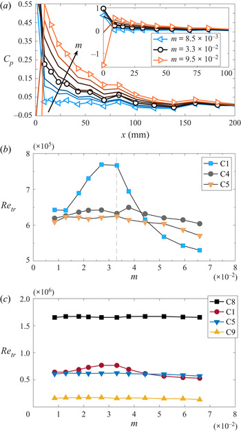


 Open access