


1. Introduction and modelling strategy
All around the world glaciers began to retreat in the second half of the 19th century and, apart from some minor interruptions, this has continued until today. In recent decades glacier retreat has accelerated and the volume loss of ice now takes place at an unprecedented rate (Zemp and others, Reference Zemp2015). There is little doubt that the rise in atmospheric temperature is the main cause for the observed glacier decline (Leclerc and Oerlemans, Reference Leclerq and Oerlemans2012; Roe, Reference Roe2011). As has been pointed out in many studies (e.g. Oerlemans and others, Reference Oerlemans1998; Mernild and others, Reference Mernild, Lipscomb, Bahr, Radić and Zemp2013), most glaciers are strongly out of balance with the current climate, and will therefore continue to retreat for decades to come, even if global warming were to slowdown. The fast retreat of glaciers is the consequence of global warming with a strong anthropogenic component (IPCC, 2013). Although this can be seen as a dramatic development, it also provides a unique opportunity to test glacier models and obtain better insights into the processes that link glacier fluctuations to climatic change.
Seen from a global perspective, the impact of changes in glacier extent and volume is mainly through a significant contribution to sea-level change (IPCC, 2013). In view of this, recent modelling efforts have focused on treating the entire glacier population on the globe (e.g. Radic and others, Reference Radić2014; Huss and Hock, Reference Huss and Hock2015). In such modelling studies, the goal is on estimating global glacier mass changes as a response to warming. Processes like accumulation, melting, calving and dynamic adjustments of glacier geometries are treated in a schematic way, involving a large number of empirical parameters to be found by tuning. Clearly, when questions of a global nature have to be dealt with, global models are needed in which not every single glacier can be treated in detail.
On a regional and local scale, glacier fluctuations may have a large effect on the security of infrastructure and buildings (ice avalanches, outbursts of glacial lakes), meltwater supply (reservoirs, irrigation) and the tourist industry (ski areas, attractiveness of alpine scenery). Retreating glaciers leave behind deglaciated terrain that is unstable (Haeberli, Reference Haeberli2017), and a new field of research is now evolving in which the formation of new landscapes is studied (Haeberli and others, Reference Haeberli, Schaub and Huggel2017). In view of this, modelling studies of individual glaciers are needed to determine the impact of different climate change scenarios and how fast the transformation of a glacierized landscape may take place.
Our modelling target is a single glacier (Vadret da Tschierva, Switzerland). In the light of recent studies in which large ensembles of glaciers are modelled in a single sweep (e.g. for the European Alps; Zekollari and others, Reference Zekollari, Huss and Farinotti2019), this may appear out of date. However, we take a different approach in model calibration by using data going back in time until 1850. This implies a more challenging model test than considering only the last three or four decades, during which glacier retreat and atmospheric warming just ran parallel (at least in central Europe). Using output from climate models to force glacier models for future projections is quite popular now, but little effort has been done to see if this works for the past 150 years. We use the output from Coupled Model Intercomparison Project 5 (CMIP5) climate simulations, starting in 1870, to investigate this point.
The Vadret da Tschierva (Vd Tschierva) is a 4 km long valley glacier in the Swiss Alps and descends from the same mountain (Piz Bernina, 4049 m) as the well-studied Vadret da Morteratsch (Vd Morteratsch; e.g. Zekollari and others, Reference Zekollari, Huybrechts, Fürst, Rybak and Eisen2013; Oerlemans and others, Reference Oerlemans, Haag and Keller2017). Maps of the Bernina region, produced in 1877 as part of the ‘Siegfriedkarte’ (https://map.geo.admin.ch/), show the extent and morphology of glaciers and their surroundings in great detail. Many historical photographs exist, allowing a good comparison with the more recent state of the glacier (Fig. 1). The length record of the Vd Tschierva glacier is shown in Figure 2, together with the record of the Vd Morteratsch. In the official dataset of the Swiss Glacier Monitoring Network, the Vadret da Roseg has a much longer length record than the Vd Tschierva. Because these glaciers merged until ~1940, the nomenclature is somewhat confusing. From many historical photographs, it is obvious that the Vd Tschierva advanced into the Val da Roseg, and that it was little affected by the Vadret da Roseg. However, in the Siegfried map of 1877, the lower part of the Vd Tschierva is actually referred to as the Vadret da Roseg, which is not logical with respect to the actual glacier dynamics. Therefore, as has been done in Oerlemans (Reference Oerlemans2012), in this study the older data points on glacier length are assigned to the Vd Tschierva instead of the Vadret da Roseg. In this way, a consistent length record for the Vd Tschierva is obtained. It should be noted that the very rapid decrease in glacier length of the Vd Morteratsch during recent years (arrow in Fig. 2) is related to the fact that the glacier front withdrew over a rock step (riegel) in the bed.
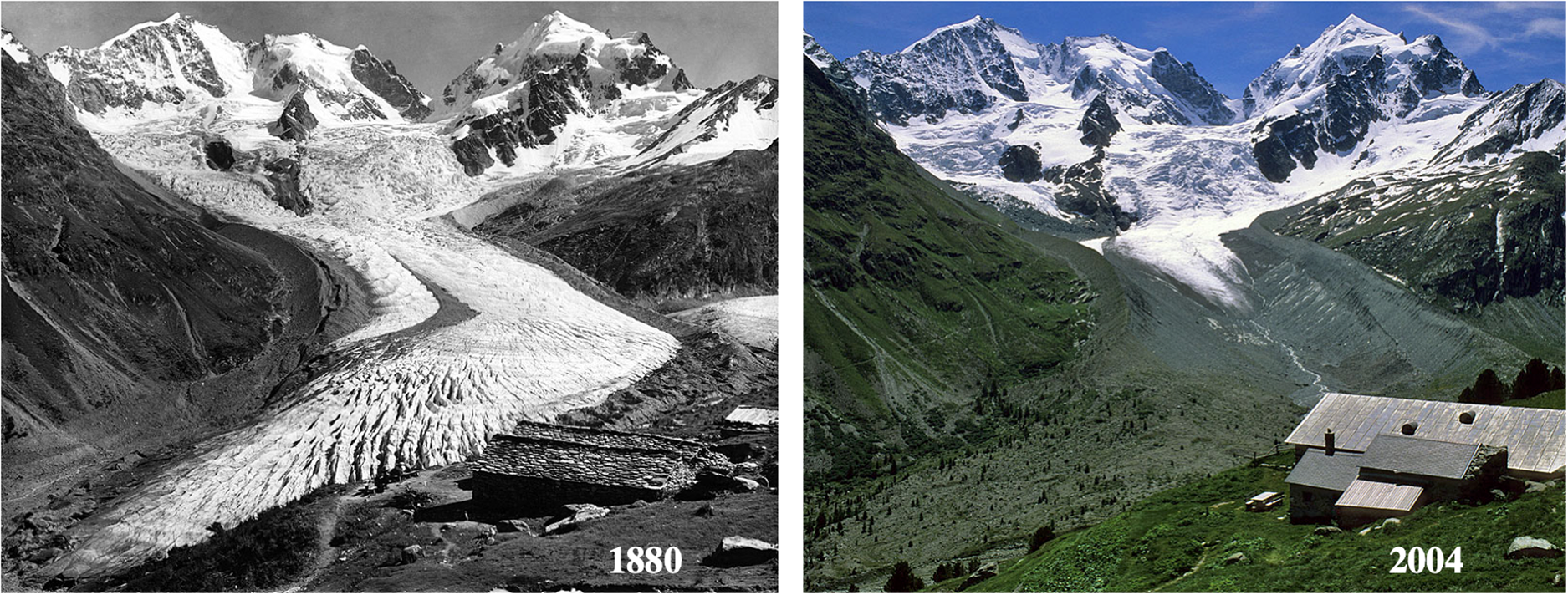
Fig. 1. The Vd Tschierva in 1880 (Alpines Museum der Schweiz) and in 2004 (J. Alean), photographed from Margun da l' Alp Ota, 2257 m a.s.l. The peak on the left is Piz Bernina (4049 m), on the right Piz Roseg (3973 m). The subsidiary moraine on the right in the 2004 photo represents the limit of the 1967–87 advance. For further images see also https://swisseduc.ch (‘Glaciers online’ by J. Alean and M. Hambrey).
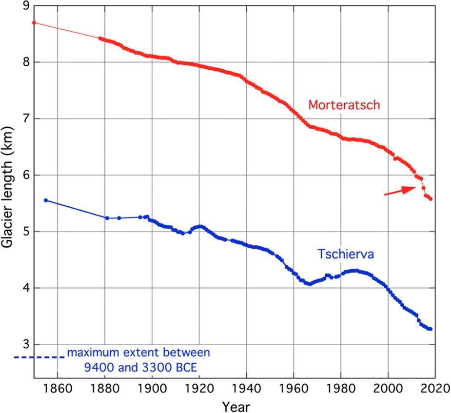
Fig. 2. Glacier length records of the Vadret da Morteratsch and the Vadret da Tschierva in the Bernina mountains. Data from the Swiss Glacier Monitoring Network with some additions and amendments as explained in the text. The last data points in this graph refer to 2018. The dashed line in the lower-left corner indicates the inferred glacier length during three Holocene Optimum Events (Joerin and others, Reference Joerin, Nicolussi, Fischer, Stocker and Schlüchter2008).
Since the maximum stand around the middle of the 19th century, the Vd Morteratsch has become ~3 km shorter and the Vd Tschierva retreated ~2 km. During periods of reduced retreat of the Vd Morteratsch, the Vd Tschierva advances to reach relative maximum stands ~1920 and 1988. With a linear inverse modelling technique, it has been demonstrated that the differences in the length records can be attributed to differences in response time (the optimal values being 9 a and 38 a, respectively, for Tschierva and Morteratsch; Oerlemans, Reference Oerlemans2012). However, this modelling technique does not reveal the cause of the difference in response times, but it seems likely that the difference in mean surface slope (the Vd Tschierva is steeper) plays a role. One of the goals of this study is to treat the fairly complex glacier geometry in more detail and to see to what extent the geometry affects the sensitivity to climate change.
Some information is also available about the former extents of the Vd Tschierva in early- and mid-Holocene times. Joerin and others (Reference Joerin, Nicolussi, Fischer, Stocker and Schlüchter2008) have studied the subglacial sedimentary archive in detail, analysing a large number of wood fragments as well as sediments in a nearby lake. According to their climatological interpretation, the glacier length never exceeded 2.7 km between 9400 and 3300 BCE (indicated in Fig. 2 by the dashed line). [Note: the absolute values of glacier length given in Joerin and others (Reference Joerin, Nicolussi, Fischer, Stocker and Schlüchter2008) differ somewhat from those referred to here, due to a slightly different definition of the major flowline]. It should also be noted that in 1988 a rockfall occurred on the ablation zone of the northeastern branch (FL2 in Fig. 3). The debris has travelled downwards and as a result, the snout of this branch is currently covered. However, it is not in active contact anymore with the southwestern flowline (FL1 in Fig. 3), i.e. not delivering mass to this flowline.
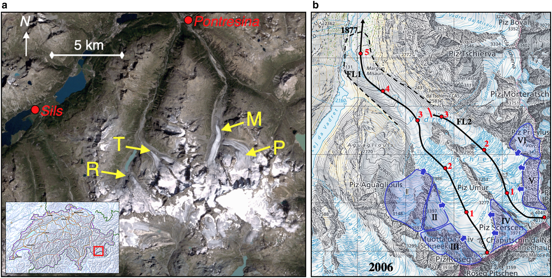
Fig. 3. (a) Landsat image (31 August 2009) of the Bernina mountains in southeast Switzerland. T: Vadret da Tschierva; R: Vadret da Roseg; P: Vadret Pers; M: Vadret da Morteratsch;. The red dot indicates the location of the Sils / Segl-Maria weather station. (b) Topographic map of the Vd Tschierva with the major and secondary flowline used in the model. Numbers in red indicate distance along the flowline in km. The blue shaded basins contribute mass to the flow lines as long as their net mass budgets are positive. The margin of the glacier tongue in 1877 is indicated by the dashed line. Courtesy of Bundesamt für Landestopografie, Köniz, Schweiz (2006).
2. Glacier model
The glacier model used in this study has several components. The ice flow model is described only briefly because it has been documented in other papers. We pay special attention to the derivation of the bed profile for the flowlines, as well as to the treatment of steep slopes that deliver mass to the main glacier by ice avalanching from hanging glaciers or directly by snow avalanches.
2.1. Ice flow model
The model used in this study is a multi-flowline model based on the Shallow Ice Approximation (SIA, e.g. van der Veen, Reference van der Veen2013). The SIA is a powerful method to study the evolution of land-based valley glaciers. The local ice velocity is determined by the local surface slope and ice thickness, making the model computationally very efficient as compared to a Full Stokes Model (FSM). This is essential because the modelling strategy employed here involves an optimization procedure that requires hundreds of simulations to be carried out. In mountain terrain, it is often feasible to calculate the glacier properties along one or more flowlines, with an appropriate parameterization of the 3-dimensional (3-D) topography. In this way, the difficulties involved in the formulation of boundary conditions for 3-D models can be avoided.
Flowline models based on the SIA have been used successfully for a long time (e.g. Budd and Jenssen, Reference Budd and Jenssen1975; Huybrechts and others, Reference Huybrechts, de Nooze, Decleir and Oerlemans1989; Oerlemans, Reference Oerlemans1997; Schmeits and Oerlemans, Reference Schmeits and Oerlemans1997; Anderson and others, Reference Anderson, Lawson and Owens2008; Oerlemans and others, Reference Oerlemans, Haag and Keller2017; Maussion and others, Reference Maussion2019). In comparison to higher-order models, some of the glacier mechanical processes are not included in the SIA (notably the effect of longitudinal stress gradients). However, in several studies, it has been shown that for the simulation of valley glaciers this is not a problem (e.g. Leysinger Vieli and Gudmundsson, Reference Leysinger-Vieli and Gudmundsson2004). With the SIA it is also relatively easy to use multiple flowlines that are coupled. The effect of tributary glaciers can then be treated in a consistent way; even when a tributary glacier withdraws from the main stream, its evolution in time can still be simulated. In their modelling study of the Pasterzenkees (Austria), Zuo and Oerlemans (Reference Zuo and Oerlemans1997) used a system with seven flowlines.
The evolution of the glacier system is described by the conservation of mass (or volume, if ice density is considered to be constant). For a flowline model, the vertically and laterally integrated continuity equation reads:

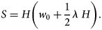
Here S is the area of the glacier cross section, U is the mean ice velocity (along the flowline) in the cross section, $\dot{b}$ is the balance rate and W is the glacier width at the surface. The x-axis is defined along the flowline in map projection; it is not a straight line but follows the flow direction of the ice. Cross sections for flowline mode have been parameterized with a trapezoidal shape (e.g. Stroeven and others, Reference Stroeven, van de Wal, Oerlemans and Oerlemans1989; Oerlemans, Reference Oerlemans1997) or a parabolic shape (e.g. Huybrechts and others, Reference Huybrechts, de Nooze, Decleir and Oerlemans1989). In this study we use the trapezoidal shape; the relation between S and H (ice thickness at the centre line) is then given by:
Here the parameter λ is determined by the surface width relative to the width of the bed (w 0):

Note that λ and w 0 vary along the flowline and thus depend on x.
The further mathematical formulation and numerical implementation of the SIA flowline model with a trapezoidal cross section has been described in earlier publications (e.g. Oerlemans, Reference Oerlemans1997, Reference Oerlemans2001) and is not repeated here.
2.2. Geometry
The major flowline (FL1) and secondary flowline (FL2) defined for the model are shown in Figure 3, together with six basins/slopes, numbered I to VI, that supply mass whenever they have a positive budget. The glacier state as mapped by the ‘Siegfriedkarte’ from 1877 has also been taken into account when defining the flowlines. The maximum length along FL2 is 3.3 km; all mass passing through this point (as determined by the local slope and thickness) is added to FL1. The dimensions of the basins as estimated from the topographical map are listed in Table 1. Actually, they can be recognized in the photographs of Figure 1.
Table 1. Characteristics of the ‘buckets’ that supply mass to the main flowline of the Vd Tschierva
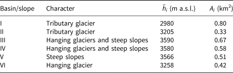
The buckets are shown in Figure 3.
Before proceeding a note on the term ‘flowline’ is in order. A flowline is normally drawn perpendicular to the isohypses because the direction of the ice movement is determined by the driving stress, and thus by the surface slope. However, in flowline models, in which mass continuity is essential and varying width has to be taken into account, it would be better to speak about flowband models. The geometric and ice mechanical properties are supposed to represent mean values in a cross section perpendicular to the axis of flow. So, for instance, FL2 is drawn across a rock outcrop at x = 1.4 km (Fig. 3), simply because it is in the middle, but the corresponding grid points represent the whole width of the glacier.
The bed topography of the Vd Tschierva is not well known. Only a few GPR measurement have been carried out in the past on the glacier tongue (Joerin and others, Reference Joerin, Nicolussi, Fischer, Stocker and Schlüchter2008). These measurements are not sufficient to derive a bed profile for the glacier flowlines to be used here. Methods have been developed to determine ice thickness from surface data based on a so-called diagnostic slope approach (for a review see Farinotti and others, Reference Farinotti2017), or with an iterative dynamic approach in which a glacier model is run repeatedly with a prescribed climatic forcing (e.g. van Pelt and others, Reference van Pelt2013). Slope-based methods (SB-method) assume that ice always behaves perfectly plastic, implying that the product of surface slope and ice thickness is constant. From a prescribed yield stress τ 0 the ice thickness can then be determined directly from the surface slope ∂h/∂x:
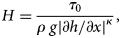
where ρ is ice density and g is the gravitational acceleration. We have introduced an empirical parameter κ to allow a better fit with observed bedrock data. For the common approach based on the assumption of perfect plasticity κ = 1. Irrespective of the validity of the physical principle, a large uncertainty in using the SB-method is related to the choice of the yield stress. The driving stress normally decreases towards the glacier head and glacier snout (Oerlemans, Reference Oerlemans2001; Fig. 6.4), implying that here the ice thickness is overestimated. It appears that SB-methods produce useful estimates of ice thickness and ice volume for regional and larger scales, but should be applied with care when the interest is in the bed profiles of individual glaciers (Farinotti and others, Reference Farinotti2017).
Paul and Linsbauer (Reference Paul and Linsbauer2011) have analysed the SB-method in some detail for the Bernina glaciers, including the Vd Tschierva. Comparing their results with observed ice thickness for the Morteratsch/Pers glacier system reveals that overall the method gives satisfactory results, but in regions where the surface slope is small, the associated bed depressions appear to be too deep. Therefore, it may be worthwhile to correct the SB-method for the Vd Morteratsch and then apply it to the Vd Tschierva to derive bed profiles for FL1 and FL2. In a recent modelling study for the Vd Morteratsch with a flowline model, a steady-state profile was calculated for the 1860 glacier stand (Oerlemans and others, Reference Oerlemans, Haag and Keller2017), using the measured bed profile described in Zekollari and others (Reference Zekollari, Huybrechts, Fürst, Rybak and Eisen2013). This glacier surface profile is a good case for testing the SB-method because transient effects are then excluded. We focus on the region between 3 and 6 km along the major flowline of the VdM because here a major and minor overdeepening occur (Fig. 4). The standard SB-method was used with κ = 1, and the value of the yield stress was found by minimizing the difference between the observed and reconstructed bed profile [yielding τ 0/(ρ g) = 15.8 m]. The RMS-difference between the resulting bed profile (dashed line in Fig. 4) and the observed profile is 30.5 m. Notably, the depth of the major overdeepening, defined as the difference between bed elevation at x = 3.7 km and at x = 4.7 km, is overestimated by 64 m. Some experimentation revealed that a better result can be obtained by adjusting κ. With κ = 0.7, the RMS-difference between observed and reconstructed profile (blue curve in Fig. 4) is only 4.6 m. Because there is a chance that the optimal value of κ varies greatly from glacier to glacier, we performed a secondary test on a flowline of the Vadret Pers (not shown). Again, a smaller value of κ produced a better result, the optimum value being 0.62.
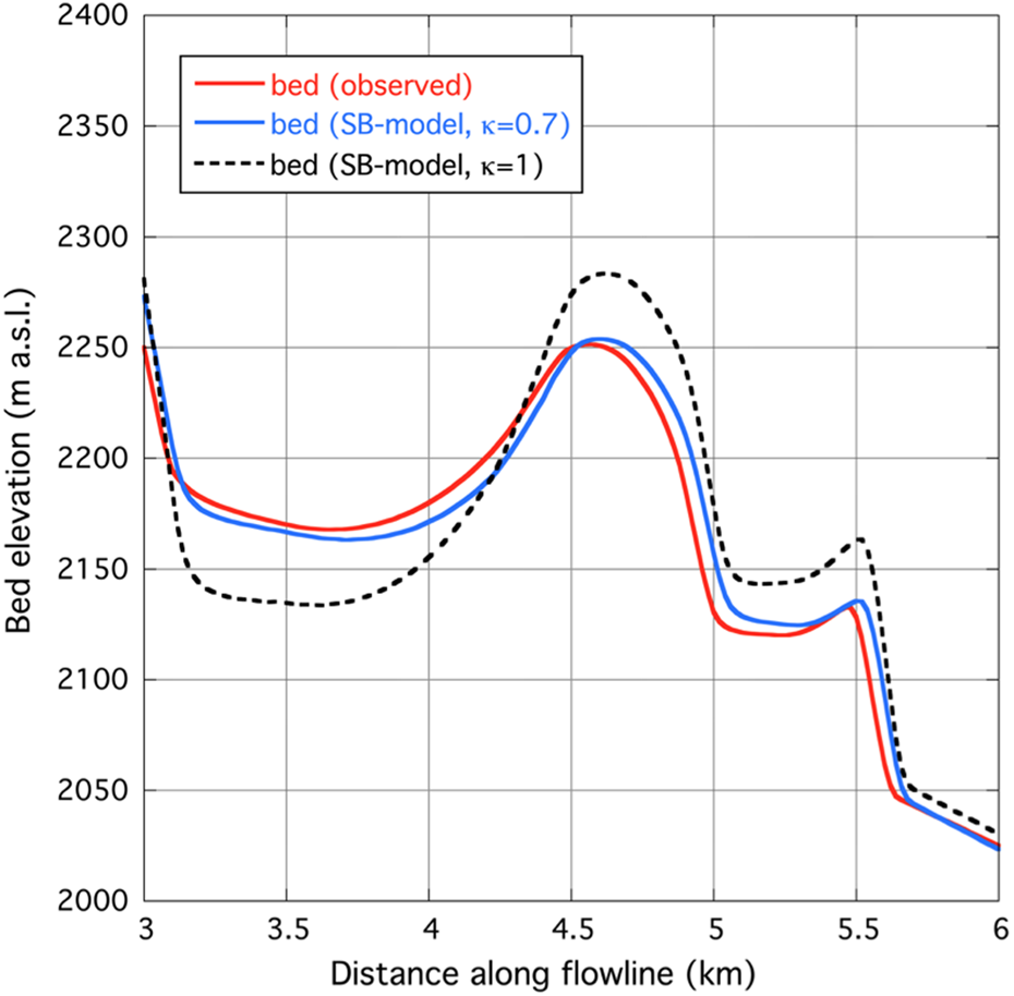
Fig. 4. Bed profiles along the central flowline of the Vd Morteratch as measured by radar (red curve), and estimated by an optimized slope-based model with different values of κ as defined in Eqn (4).
Altogether we decided to reconstruct the bed profiles for FL1 and FL2 of the Vd Tschierva with κ = 0.7 (Fig. 7a). Later in this paper, we will evaluate the importance of undulations in the bed by making a comparison with a simple piece-wise linear representation of the glacier bed.
The parameters describing the cross profiles were estimated from the topographic map. For the part of the flowlines currently covered by ice this involves some ambiguity. However, the surface width should be predicted correctly by the model, which serves as a constraint. It should be noted that even within a time span of a few centuries the profiles may change significantly. For instance, the almost perfect V-shape observed between km 3.5 and km 4.5 of FL1 most likely originated from the formation of the side moraines during the retreat from the maximum stand in the middle of the 19th century. As a result, there is an unquantified uncertainty in the values of λ and w 0.
2.3. Balance rate
The balance rate is prescribed according to an altitudinal profile, with the same parameter values as used in the modelling study of the Vd Morteratsch (Oerlemans and others, Reference Oerlemans, Haag and Keller2017):
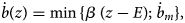
where β is the balance gradient $( 0.0065\;{\rm m\;w}{\rm .e} .\;{\rm m}^{ \hbox{-} 1}{\rm a}^{ \hbox{-} 1})$ and $\dot{b}_m$
 an upper limit to the balance rate $( 3\;{\rm m\;w}{\rm .e}{\rm .\;}{\rm a}^{ \hbox{-} 1})$
 . E is the equilibrium-line altitude and z is height above sea level. The application of an upper limit for the balance rate has a rather limited effect because the area involved is very small. The climatic forcing of the glacier model operates through the time dependency of E.
The supply of mass from the tributary basins/slopes occurs through a variety of processes, which are not easy to quantify. A substantial part of the snow falling on these basins will find its way to the flowlines by means of avalanches. Slope V (Fig. 3) is the most extreme case. Because of its steepness, it does not build up perennial snow or ice, and here we simply assume that all the mass gain is delivered to FL2 instantaneously. For the basins (index i) depicted in Figure 3 the net mass budget B i is written as

where A i is the area of basin i and $\bar{h}_i$ its mean surface elevation. Eqn (6) is only valid when there is no upper limit to the balance rate. This has been done to avoid that the balance rate has to be integrated over the precise hyposometry of the basins for every different value of E. Instead, a somewhat smaller value of β is used $( 0.005\;{\rm m\;w}{\rm .e} .\;{\rm m}^{ \hbox{-} 1}{\rm a}^{ \hbox{-} 1})$
 .
.
3. Simulation of the historical length record
One way to calibrate a glacier model is to determine the climate forcing that delivers the smallest RMS difference between observed and simulated glacier length (RMS L). Here this is achieved by starting with a first-guess forcing function E (t), which has different values of E for 5-year periods (E 5). Then a particular value of E 5 is perturbed, the model is run and the new value of RMS L is calculated. When this value is smaller, the new value of E 5 is kept, otherwise, it is rejected. By marching through the period of simulation in a quasi-random manner, a minimum value of RMS L is ultimately achieved. The result of this procedure, which requires hundreds of runs, is shown in Figure 5. It should be noticed that the model has been initialized by running it to a steady state that corresponds to the LIA (Little Ice Age) maximum stand (mid-19th century). The corresponding value of the equilibrium-line altitude appears to be 2888 m. There is no hard evidence that ~1850 the glacier was close to a steady state, but it is probably the best assumption one can make.
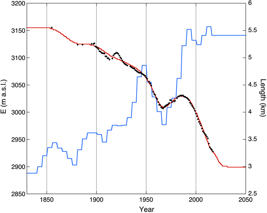
Fig. 5. Optimized simulation of the historical record of the Vd Tschierva. The length observations are shown as black dots, the red line represents the simulated length (scale at right). The reconstructed equilibrium-line altitude is shown in blue (scale at left).
Our results suggest that a rise of the equilibrium line of ~250 m since 1850 is needed to explain the retreat of the Vd Tschierva. Superimposed on this trend is a major depression in the ELA between 1950 and 1980, leading to the maximum glacier stand ~1985. The minor advance recorded ~1920 cannot be reproduced by the model. The timescale of this fluctuation is too short to be recovered, unless the forcing would be set to unrealistical values. When the value of E is kept constant after 2015, and equal to the 2001–15 mean value, the model glacier approaches a steady state ~2025, with a length of 3 km. Later we will discuss integrations until 2100 for different climate change scenarios. Some longitudinal profiles along FL1 are shown in Figure 6.
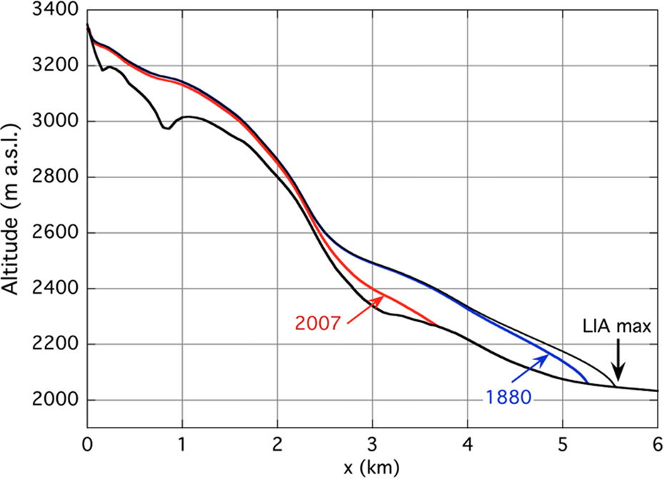
Fig. 6. Bed and surface profiles for FL1. The surface profiles for 1880 and 2007 correspond to the photographs in Figure 1.
The years correspond to the photographs in Figure 1. For x < 2.3 km the difference in ice thickness between the two profiles is small. Currently, the glacier snout is close to the kink in the bed profile at x ≈ 3 km. Some further model experiments revealed that this kink has a significant effect on the dimensionless climate sensitivity γ L of the glacier length L, defined as

where L E is the equilibrium glacier length corresponding to the value of E. For L > 3 km the value of γ E is ~10, and for L < 2 km it is ~5 (with transitional values in between). At the same time, the e-folding response time appears to be smaller for smaller values of L (ranging from ~5 to ~35 years).
To find out how important the details of the bed profiles of FL1 and FL2 are for the long-term dynamics of the glacier, we have carried out some numerical experiments with a piecewise linear representation of the bed (Fig. 7a). In these experiments, the undulations in the bed profile have been removed, and the model was run with the reconstructed ELA as forcing for the period 1850–2020. In Figure 7b glacier length is shown for the standard run, for a run with the linear approximation of the bed profile for FL2 only, and for a run with linear bed approximation for FL1 and FL2. Apparently, the differences are rather small. However, they become larger towards the end of the simulation, when the glacier tongue comes closer to the undulations in the bed. Nevertheless, we conclude that for the simulation of the historical changes of the Vd Tschierva the details of the bed profile are of minor importance.
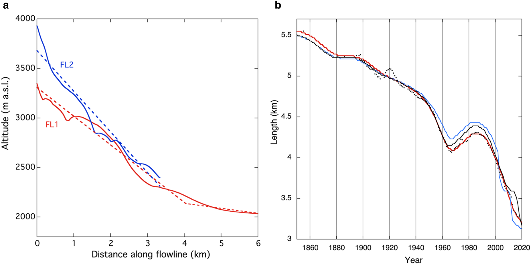
Fig. 7. (a) Bed profiles for the flow lines; the dashed lines show the linear approximation used in the sensitivity test. (b) Simulation of the glacier length for the reconstructed ELA history. The red curve represents the standard run, the blue curve a run with the linear approximation of the bed profile for FL2 only, and the black curve a run with linear bed approximation for FL1 and FL2. The black dots show observed glacier length.
It is also instructive to consider the response of the model to slow periodic forcing because it illustrates the nonlinearities related to the characteristics of the bed as well as the asymmetry between periods of advance and retreat. Figure 8a shows the length of the two flowlines for forcing with a period of 500 years and an amplitude of 400 m. The model was integrated over several cycles to remove transient effects, so the result shows the true periodic solution. Note that the value of FL2 has an upper bound (at the length where it flows into FL1). The most outstanding feature of the model response is the asymmetry between the phase of advance, which is relatively slow, and the phase of retreat, which is much faster. The retreat from L > 3.1 km to L > 2.4 km is particularly fast. This is the zone where the bed profile is steep and the ice thickness is small, notably during the retreat. To illustrate this in more detail Figure 8b shows glacier profiles during the advance and retreat for the same glacier length.
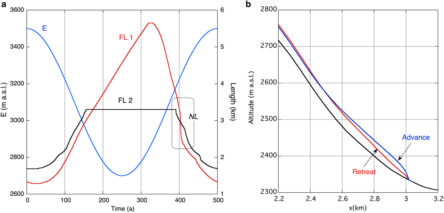
Fig. 8. (a) Length of flowline 1 (FL1) and flowline 2 (FL2) for slow periodic forcing (E, scale at left). NL stands for Non-Linear. (b) Two profiles along FL1 for a retreating and advancing glacier of the same length.
4. Comparison of ELA histories
The ELA history derived from the length variations of the Vd Tschierva can be compared to the result of a similar procedure for the Vd Morteratsch (Oerlemans and others, Reference Oerlemans, Haag and Keller2017). Due to the proximity of the Vd Morteratsch one would expect that the glaciers have been subject to almost identical climatic forcing. Figure 9 shows that this is indeed the case, at least over the past 100 years. However, the reconstructed ELA variations before 1900 are not present in the reconstruction based on the Vd Morteratsch record. It is noteworthy that the mean values of the ELAs for the Vd Tschierva and the Vd Morteratsch differ by ~130 m. This is due to the fact that in the Morteratsch study the delivery of mass from the steep slopes was not considered. In the calibration procedure, this is then compensated by a lower ELA.
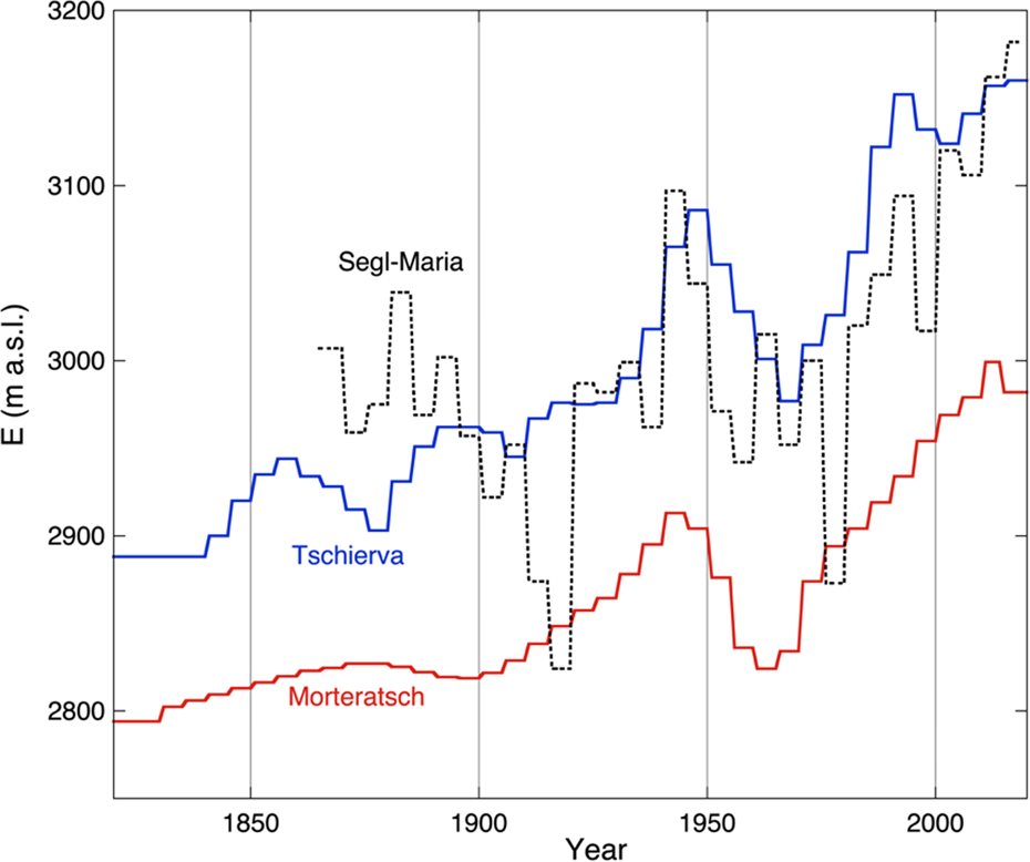
Fig. 9. A comparison of histories of the equilibrium-line latitude. The blue curve is the reconstructed history discussed in section 3. The red curve is from a model study of the Morteratsch glacier, obtained with the same control method (Oerlemans and others, Reference Oerlemans, Haag and Keller2017). The dashed curve has been calculated from the Segl-Maria meteorological record.
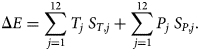
The Segl-Maria weather station has delivered a long series of meteorological observations (since 1864). The station is only ~7 km away from the Vd Tschierva. We computed an ELA history from these observations and compared it to the history reconstructed from the glacier fluctuations. To achieve this, we use the so-called Seasonal Sensitivity Characteristics (SSC), which is a 2 × 12 matrix S i,j consisting of the sensitivity of annual values of E to monthly anomalies of temperature and precipitation (Oerlemans, Reference Oerlemans2001). The index i is either T (temperature anomaly) or P (precipitation anomaly); the index j runs from 1 to 12 (month). For a year with temperature and precipitation anomalies T j and P j, the corresponding anomaly of the ELA can be calculated from:
The SSC has been obtained from a spatially distributed energy/mass-balance model that was designed for the Vd Morteratsch. It has been carefully calibrated with mass balance and meteorological observations carried out on this glacier for many years (Klok and Oerlemans, Reference Klok and Oerlemans2004; van Pelt, Reference van Pelt2010). We have assumed that the SSC for the Vd Morteratsch is also valid for the Vd Tschierva because the glaciers are so close and exposure and shading effects are rather similar. The SSC is shown in Figure 10. As expected, summer temperature and winter precipitation are the most important contributors to the annual variation in E. In fact, summer precipitation and winter temperature do not play a role at all.
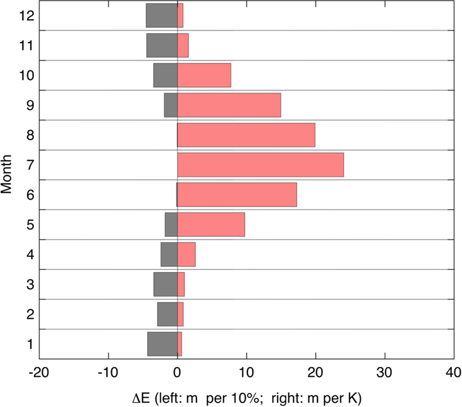
Fig. 10. Seasonal Sensitivity Characteristic for the ELA as derived from energy-balance modelling for typical Inner Alpine conditions. The red bars refer to values of ΔE for temperature perturbations in the respective months; the black bars refer to precipitation perturbation.
Applying Eqn (8) to the monthly temperature and precipitation measurements of Segl-Maria (MeteoSwiss), and calculating 5-year mean values for a better comparison, yields the dashed curve in Figure 10. There is a significant correlation of this curve with the ELA history reconstructed from the glacier fluctuations (correlation coefficient 0.67), but there are also some obvious discrepancies. Notably, the ELA decrease of ~120 m from 1915 to 1925 is not present at all in the glacier reconstructions. The decrease is mainly due to low observed summer temperatures. Overall, the contribution of precipitation and temperature anomalies to the total variability of the ELA is quite comparable. However, the rise in the ELA over the past decades is entirely due to an upward temperature trend. We have no explanation for the discrepancy between the reconstructed ELA from the glacier length record and from the meteorological data. However, we suspect that the climate series from Segl-Maria is perhaps not as ‘homogeneous’ as generally assumed. The station has been moved four times, and is located in a dynamic partly forested landscape.
We have also tried to reconstruct ELA histories from the output from global climate models, as documented in the CMIP5 (e.g. Taylor and others, Reference Taylor, Stouffer and Meehl2012). Monthly anomalies of precipitation and temperature from the nearest model gridpoint were used to compute changes in the ELA with the SSC defined above. Apart from taking anomalies relative to the period of simulation (1870–2100), no special downscaling techniques were applied. High-resolution output from Regional Climate Models (e.g. the EURO-CORDEX project) could not be used because the simulations start in 1951 or later. Of all the climate models participating in CMIP5, we have selected five of the more comprehensive models with full ocean-atmosphere coupling (CanESM2, CCSM4, CSIRO, GFDL, MPI). It appears that the interannual ELA variability is reproduced well (Std dev. between 150 and 200 m, which is in line with observations). However, on the longer timescale the correlation coefficients between the glacier-reconstructed ELA and climate model simulations are not large: 0.54, 0.62, 0.54, 0.63, 0.48, respectively. Correlation coefficients between the ELA from the Segl-Maria meteorological data and the model simulations are even lower: 0.18, 0.27, 0.13, 0.15, 0.03. The poor performance of climate models with respect to decadal temperature variations, even when averaged over larger areas, is a well-known feature (e.g. Miao and others, Reference Miao2014). It is probably more related to the uncertainty in the forcing functions (e.g. volcanism, solar activity, long-term fluctuations in ocean heat storage) than in the quality of the models themselves. In any way, it constitutes a problem when one wants to use climate projections from models to drive glacier models. Because of a glacier's memory, a projection into the future should preferably be based on a correct simulation of the past. As demonstrated in the next section, this turns out to be difficult with the climate model output referred to above.
5. The future of the Vadret da Tschierva
The most transparent way to investigate how the Vd Tschierva will respond to future climate warming is to run the calibrated model for prescribed rates of a rise of the equilibrium line. Figure 11 shows how the calibrated model responds to changes in the equilibrium line of 0, 2, 4 and 6 ${\rm m\;}{\rm a}^{ \hbox{-} 1}$ . To put this in perspective: according to the comprehensive analysis of Žebre and others (Reference Žebre2021) the change in ELA during the period 1905–2005 was between 1 and 2 ${\rm m\;}{\rm a}^{ \hbox{-} 1}$
 . From our calibration (Fig. 5) we found a value of 1.9 ${\rm m\;}{\rm a}^{ \hbox{-} 1}$
 for this period. The scenario with an ELA rise of 2 ${\rm m\;}{\rm a}^{ \hbox{-} 1}$
 would thus broadly correspond to a continuation of the climatic forcing over the past 100 years.
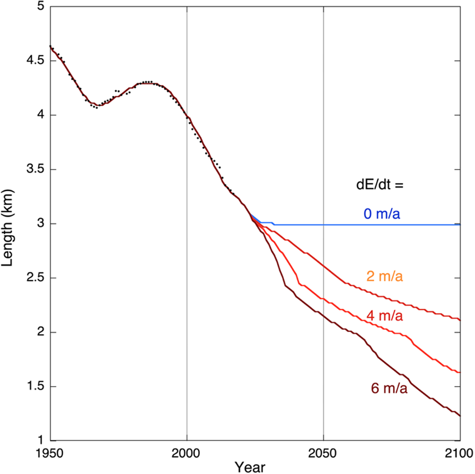
Fig. 11. Predicted glacier length for various climate change scenarios, prescribed by a steady rise of the equilibrium line as indicated by the labels.
Except for the scenario of no climate change, rates of glacier retreat are particularly high in the coming decades and slowdown afterwards. This is a geometric effect related to the bed profile. For the case with an ELA rise of 6 ${\rm \;m\;}{\rm a}^{ \hbox{-} 1}$ , which would roughly correspond to the RCP6.0 emission scenario (IPCC, 2013), not much of the Vd Tschierva is left in 2100 (length of 1.2 km). With an ELA rise of 2 ${\rm m\;}{\rm a}^{ \hbox{-} 1}$
 , which would be a reasonable value if the Paris Climate Agreement targets (UNFCCC, 2015) were met, the glacier length would be 2 km in 2100, i.e. the snout would be at the upper part of the current icefall (see Fig. 1).
It is common practice now to use the output from global or regional climate models to predict future changes in environmental systems. When these systems have substantial response times, like glaciers, the definition of an appropriate initial state is not a trivial matter. Since climate models do not reproduce patterns of climate change over the past 150 years very well, it is difficult to use the climate model simulation for calibration. This is illustrated in Figure 12, where output from the CCSM4 model has been used to drive the glacier model (for the RCP2.6 and RCP4.5 scenarios). Equation (8) has been used again to convert model output into changes in the ELA. Somehow a re-calibration had to be done to obtain a meaningful simulation. We chose to adjust the forcing in such a way that the model produces the correct present-day glacier length. To achieve this a constant value had to be added to the ELA (the 300 m step in ELA at the beginning of the integration). The resulting forcing is shown by the blue (RCP2.6) and red (RCP2.6) curves in Figure 12. The simulated glacier length shows a reasonable agreement with the observed record on the decadal timescale, but does not reproduce the trend over the past 100 years. Instead of introducing a step in the ELA one could also choose to superpose a linear trend in the ELA over the past 100 years. However, it is not clear what is to be learned from such a calculation.
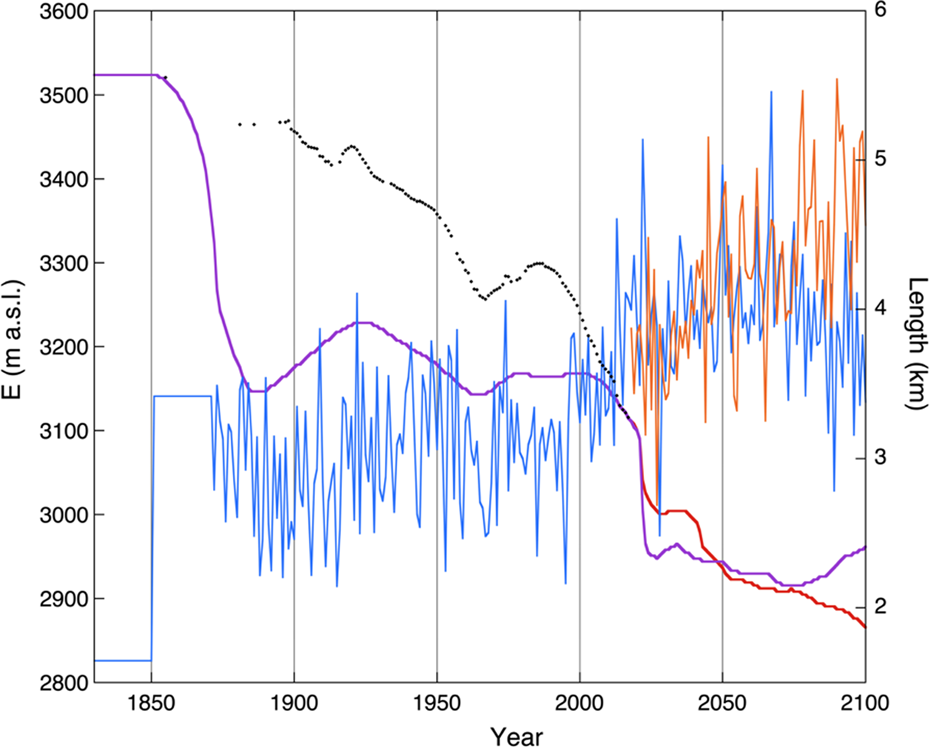
Fig. 12. Simulated glacier length (scale at right) from the model output of the RCP2.6 run (purple) and the RCP4.5 run (red) of the CCSM4 model (CMIP5). The blue curve (scale at left) represents the forcing for RCP2.6, the red curve for RCP4.5 (only shown from 2017 onwards). The black dots show the observed glacier length (scale at right).
Simulations have been carried out for all the five climate models mentioned in Section 4, and it appears that none of them is able to produce a realistic simulation of the observed glacier length record. The strong glacier retreat during the 20th century is not simulated, and the obvious reason is the lack of a steady rise in the ELA as illustrated in Figure 13.
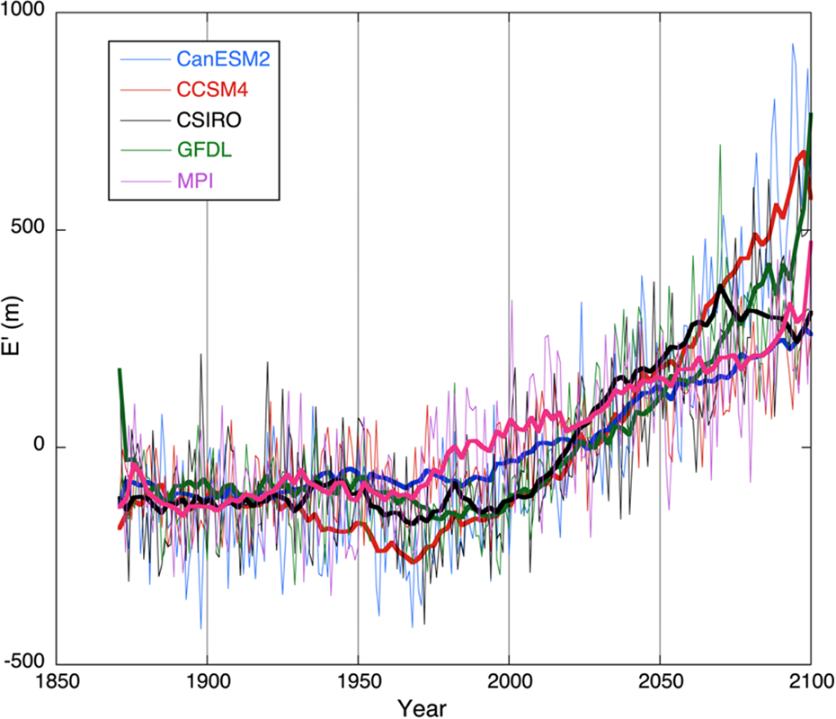
Fig. 13. Perturbation of the equilibrium line altitude (E’) for southeast Switzerland as simulated by the selection of climate models for the RCP4.5 scenario. Thin lines: annual values; bold lines: band-pass filtered.
6. Discussion
6.1 Novel points of this study
In this paper, we have used a relatively simple glacier model to study the historical fluctuations of the Vd Tschierva and investigated its possible future behaviour under various scenarios of climatic change. Novel aspects of this study are:
(i) The combination of a flowline model with ‘buckets’ to represent the mass input from hanging glaciers and steep slopes. This method appears to work well. It makes it possible to deal with mass supply from the sides without having mass-conservation problems when steep slopes are included in 3-D models. The buckets react to climate change: for a higher ELA they deliver less mass (or nothing at all) to the main stream. The underlying assumption, namely that the timescale of the hanging glaciers is significantly smaller than that of the main steam, seems quite reasonable.
(ii) The careful calibration of the model by reconstructing the ELA history from the observed glacier length fluctuations. Since this is essentially a control method in which many parameters are varied, many runs (>100) have to be carried out. The method works because the SIA model is very fast and the number of runs that can be done is basically unlimited. It is encouraging that the reconstructed ELA history compares well with that from a similar calibration exercise for the Vd Morteratsch, at least for the past 100 years.
(iii) The comparison of the reconstructed ELA history with ELA histories from local climate observations and comprehensive climate models. Here a significant discrepancy was found between the ELA history reconstructed from the glacier length and from climate data (since 1864). The climate station is not far away from the glacier, yet there is reasonable agreement only after 1930. Although the Segl-Maria climate series is officially a homogeneous series, one may doubt to what extent this applies to fluctuations on longer timescales. The station has been moved four times and is located in a dynamic landscape. With respect to ELA reconstructions from climate model data, the results are simply disappointing. None of the climate models in CMIP5 is able to reproduce the ELA history required to explain the glacier length record. The major reason for this is that these models do not reproduce the warming trend over the period 1875–1990 and consequently the long-term equilibrium line does not rise. We consider it unlikely that more sophisticated downscaling techniques will change this finding.
(iv) The notion that ‘slope-based methods’ to determine glacier thickness probably overestimate overdeepenings. For the Vadret da Morteratsch and Vadret Pers we found that the measured overdeepening is only 30 to 50% of that found from a SB-based method. We suggest that taking the surface slope to power 0.7 gives better results. This should be tested for other valley glaciers for which bed profiles have been measured.
6.2 Implications for projections of glacier extent
Perhaps the most important aspect of this study is the demonstration that making projections with output from climate models has the risk of underestimating the uncertainties. In studies in which simplified glacier models have been applied to a large set of glaciers (regional or world-wide scale), a broad agreement between simulated and observed changes has been demonstrated for the last 40 or 50 years (e.g. Radic and others, Reference Radić2014; Huss and Hock, Reference Huss and Hock2015; Zekollari and others, Reference Zekollari, Huss and Farinotti2019). However, it is still a real challenge to go further back in time. Matching observed glacier length records over the past 100 or 150 years would increase the credibility of the models used.
In making projections of future glacier changes, regional or global, the definition of the initial state remains an issue of concern, especially for systems with larger glaciers and longer response times. We suggest that the outcome of global glacier models should be tested more thoroughly against detailed studies of individual glaciers, or groups of glaciers (e.g. on Svalbard). Broadly speaking, a believable model of future glacier evolution should also be able to reproduce the LIA glacier extent in different parts of the world. Or, turning it around, the LIA glacier extent, which has been mapped around the globe, could be used to constrain and improve models in a systematic way.
Acknowledgement
We thank Roderik van de Wal (Utrecht University) for help with the CMIP5 data. We are grateful to the reviewers and the scientific editors for their careful evaluation of the manuscript and their constructive criticism.


 Open access