


1. Introduction
Since the seminal work of Reynolds, to whom we owe the ubiquitous Reynolds number, on transition to turbulence in pipes (Reynolds Reference Reynolds1883) and the discovery of the famed inflection point criterion by Rayleigh (Rayleigh Reference Rayleigh1879) that are the cornerstones for hydrodynamic stability theory, the field has seen a great deal of development. A central concept in stability analysis is to consider the linearisation of the operator or Jacobian about a base flow and compute its eigenvalues that govern whether infinitesimal perturbations will ultimately grow or decay. This approach has had tremendous success in the analysis of the asymptotic fate of perturbations in steady parallel flows from the early solution of the Rayleigh–Bénard convection (Rayleigh Reference Rayleigh1916) to the analysis of the viscous linear stability of parallel flow leading to the Orr–Sommerfeld (OS) operator (Orr Reference Orr1907; Sommerfeld Reference Sommerfeld1908) that has been the object of numerous analytical and numerical studies (Orszag Reference Orszag1971; Drazin & Reid Reference Drazin and Reid1981). Despite the progress, it was only relatively recently that the persistent mismatch between the predicted onset of linear instability in many shear flows and the experimental and numerical evidence of transition at much lower Reynolds numbers (Klebanoff, Tidstrom & Sargent Reference Klebanoff, Tidstrom and Sargent1962; Avila et al. Reference Avila, Moxey, de Lozar, Avila, Barkley and Hof2011) was explained. In fact, for non-normal operators such as the linearised Navier–Stokes operator, the focus on its spectrum alone blinds the investigation for growth mechanisms exploiting the non-orthogonality of its eigenbasis; instead, the pseudospectra need to be analysed (Reddy & Henningson Reference Reddy and Henningson1993; Trefethen et al. Reference Trefethen, Trefethen, Reddy and Driscoll1993). This new perspective on the stability of fluid flow puts the focus on transient amplification of initial disturbances to levels at which nonlinear effects take over that bypass the modal path to turbulence (Henningson, Lundbladh & Johansson Reference Henningson, Lundbladh and Johansson1993). This realisation has led to the development of non-modal stability theory that centres the analysis on a linear initial value problem avoiding the restrictions imposed by the normal mode ansatz. For a detailed review on the topic see Schmid (Reference Schmid2007). Besides linear stability methods, a number of approaches based on nonlinear theory have been developed. For a recent review on these methods see Kerswell (Reference Kerswell2018).
In recent years, with the increased availability of computer power, global instability theory has gained interest (Huerre & Monkewitz (Reference Huerre and Monkewitz1990), see Chomaz (Reference Chomaz2005) or Theofilis (Reference Theofilis2011) for reviews of recent developments). This method does not rely on spatial homogeneity of the flow, allowing for much more geometric flexibility at the cost of larger computations that require specialised tools (Theofilis Reference Theofilis2003). The combination of the linear stability analysis framework with matrix-free timestepping methods routinely used in flow solvers (Barkley, Blackburn & Sherwin Reference Barkley, Blackburn and Sherwin2008; Bagheri et al. Reference Bagheri, Åkervik, Brandt and Henningson2009a) has paved the way for global stability and transient growth analyses of increasing complexity and fidelity (Blackburn, Barkley & Shervin Reference Blackburn, Barkley and Shervin2008; Monokrousos et al. Reference Monokrousos, Åkervik, Brandt and Henningson2010; He et al. Reference He, Tendero, Paredes and Theofilis2017; Tsigklifis & Lucey Reference Tsigklifis and Lucey2017; Chauvat et al. Reference Chauvat, Peplinski, Henningson and Hanifi2020).
A common feature of most of the studied flow cases is that, despite the spatial complexity, they rely on a steady base flow in order to perform the stability analysis. This limits the direct application of the methods to sub-critical Reynolds numbers where flows are naturally stable (Mack & Schmid Reference Mack and Schmid2011; He et al. Reference He, Tendero, Paredes and Theofilis2017). In unstable scenarios, it requires artificial stabilisation methods to recover a steady base flow such as fixed-point iterations (reviewed in Knoll & Keyes Reference Knoll and Keyes2004) or relaxation term methods such as selective frequency damping (Åkervik et al. Reference Åkervik, Brandt, Henningson, Hæpffner, Marxen and Schlatter2006; Loiseau et al. Reference Loiseau, Robinet, Cherubini and Leriche2014; Chauvat et al. Reference Chauvat, Peplinski, Henningson and Hanifi2020) or, for oscillating flows, the use of time-averaged data (Hammond & Redekopp Reference Hammond and Redekopp1997). In fact, unsteady flows are notoriously challenging to analyse and progress in the understanding of their linear stability characteristics has been slow (Schmid & Henningson Reference Schmid and Henningson2001). Significant steps towards this goal have been made only for time-periodic flows using energy theory (Davis & Von Kerczek Reference Davis and Von Kerczek1973), non-modal stability analysis (Xu, Song & Avila Reference Xu, Song and Avila2021) and especially Floquet theory (Davis Reference Davis1976). The latter transforms the time-periodic problem into a linear eigenvalue problem by assuming periodic solutions of the same frequency as the base flow that can be solved with standard stability tools for steady states. While this technique has been applied to a wide range of flows (Von Kerczek Reference Von Kerczek1982; Barkley & Henderson Reference Barkley and Henderson1996; Marques & Lopez Reference Marques and Lopez1997; Pier & Schmid Reference Pier and Schmid2017), it has the fundamental shortcoming that, although it distinguishes between stable and unstable flows in the time-asymptotic limit, it ignores intracyclic growth and decay that can be substantial enough to trigger turbulence via nonlinear mechanisms.
Recently, the optimally time-dependent (OTD) modes have been proposed as a new framework for the analysis of linear perturbations in time-dependent systems (Babaee & Sapsis Reference Babaee and Sapsis2016). The method generates a time-evolving orthonormal basis of a finite-dimensional subspace around an arbitrary time-dependent trajectory that spans the instantaneously most unstable directions of the tangent space. Following their proposal, a series of works have established a number of characteristics of the OTD modes. In particular, it was shown that they converge exponentially fast to the most unstable eigendirections of the Cauchy–Green tensor, making them well suited for the reduced-order computation of finite-time Lyapunov exponents (Babaee et al. Reference Babaee, Farazmand, Haller and Sapsis2017), and that they are identical to continuously orthonormalised Gram–Schmidt vectors for a specific choice of parameters (Blanchard & Sapsis Reference Blanchard and Sapsis2019a), which has proved to be a relevant connection for the application of OTD modes. The strength of the OTD basis vectors is their capacity to span the instantaneously most unstable subspace of user defined size in the (possibly infinite-dimensional) phase space and to capture both modal and non-modal growth within that subspace. Furthermore, the OTD basis vectors are flow invariant (Babaee & Sapsis Reference Babaee and Sapsis2016) and are dynamically consistent with the full dynamics (Farazmand & Sapsis Reference Farazmand and Sapsis2016; Blanchard, Mowlavi & Sapsis Reference Blanchard, Mowlavi and Sapsis2018). These characteristics have led to several applications ranging from control of linear instabilities (Blanchard et al. Reference Blanchard, Mowlavi and Sapsis2018; Blanchard & Sapsis Reference Blanchard and Sapsis2019c), prediction of dynamical events in a statistical framework (Farazmand & Sapsis Reference Farazmand and Sapsis2016), the computation of sensitivities (Donello, Carpenter & Babaee Reference Donello, Carpenter and Babaee2020) to edge tracking (Beneitez et al. Reference Beneitez, Duguet, Schlatter and Henningson2020), leveraging the ability of the OTD modes to follow the linear dynamics even along a chaotic trajectory.
In these works, the OTD basis was used primarily as a stable and efficient numerical tool to obtain a basis of the most unstable subspace, but the structure of the OTD modes themselves has not been in the focus. In fact, a linearisation around a complex, nonlinear state makes the physical interpretation of the OTD modes difficult. In order to develop a better understanding of the physical relevance of the OTD modes, it is useful to apply the framework to a simpler case in which the base flow is better understood. A good candidate for this purpose is pulsating Poiseuille flow. In this canonical time-periodic parallel flow configuration, the constant pressure gradient of plane Poiseuille flow is modulated harmonically around the mean. Due to the geometric simplicity, the availability of a general analytical solution of the incompressible Navier–Stokes equations for the base flow and the wealth of data in the literature, especially on its Floquet stability, this flow case is ideal as a benchmark for transient linear stability analysis using the OTD framework. In particular, the configuration is not only unsteady but non-autonomous via the forced pressure oscillations making its instantaneous stability properties entirely inaccessible to linear stability analysis via the global mode approach.
The aim of this paper is to give an overview of the theoretical understanding of the OTD framework and to illustrate its potential as a general tool for the linear stability analysis of time-dependent flows, in particular for time-periodic configurations. The general purpose implementation in the spectral element code Nek5000 (Fischer, Lottes & Kerkemeier Reference Fischer, Lottes and Kerkemeier2008) is applied to pulsating Poiseuille flow to feature the capabilities and assess the limitations of the method in order to provide a guide for the application of the framework to other flow cases. The instantaneous growth rates and spatial structure of the OTD modes are analysed, the interaction between pulsation and non-normal growth potential is explored and the existence of subharmonic perturbation cycles is documented.
The remainder of this paper is organised as follows. In § 2 we review the OTD framework theory before introducing the formulation for the incompressible Navier–Stokes equations used in this work (§ 3). We then introduce the flow case used to illustrate and validate the implementation in Nek5000 (§ 4) and present the results of the transient linear stability analysis based on the OTD modes (§ 6). A discussion of the main findings and concluding remarks are gathered in § 7.
2. OTD modes
2.1. Problem specification
We consider a general  $n$-dimensional dynamical system
 \begin{equation} \frac{\partial z}{\partial t} = f(z,t),\quad z \in \mathbb{R}^{n},\enspace t \in [t_0, t_0 + T], \end{equation}
where  $f : \mathbb {R}^{n} \times [t_0, t_0 + T] \to \mathbb {R}^{n}$ is a nonlinear but sufficiently smooth vector field. We denote by $z(t):=z(t,z_0,t_0)$ a solution of (2.1) with the initial conditions $z(t_0) = z_0$ as the state of a trajectory of the system at time $t$. Infinitesimal perturbations $q(z(t),t)$ about the nonlinear trajectory $z(t)$ are governed by the linearised dynamics
 \begin{equation} \frac{\partial q}{\partial t} = L(z(t),t) q,\quad q \in \mathbb{R}^{n},\enspace \mbox{with}\ L(z(t),t) := \boldsymbol{\nabla}_z f(z(t),t), \end{equation}
where  $L(z(t),t)$ is the Jacobian of the vector field $f$.
$f$.
The general solution of (2.2) can be expressed using the propagator  $\boldsymbol {\nabla } F_{t_0}^{t}$ that maps the perturbations at the initial time $t_0$ to $t$ along the linearised dynamics given by
 \begin{equation} q(t) = \boldsymbol{\nabla} F_{t_0}^{t} q_0, \end{equation}
where  $q_0 = q(t_0)$.
2.2. Preliminaries
When analysing systems of the form (2.2) for their stability properties, the dominant direction of the tangent space is easily recovered e.g. via the impulse response technique. If the goal is to also extract information about subdominant directions, the naive approach to simply integrate a set of vectors using the equations in time is in general doomed to fail. In practice, almost all initial conditions will asymptotically align with the most unstable direction while their magnitude grows or decays exponentially, leading to numerical instability and large errors (Wolf et al. Reference Wolf, Swift, Swinney and Vastano1985). In order to avoid both the collapse of all perturbations onto the least stable direction as well as numerical over/underflow, the OTD modes were introduced in Babaee & Sapsis (Reference Babaee and Sapsis2016) by including an orthonormality constraint into the linear evolution equations. The resulting evolution equations for the OTD basis vectors  $q_i$ for $i=1,\ldots ,r$ are given by
 \begin{equation} \frac{\partial q_i}{\partial t} = Lq_i - \sum_{j=1}^{r} \left( \langle Lq_i, q_j \rangle - \varPhi_{ij} \right) q_j ,\end{equation}
where  $\langle \cdot , \cdot \rangle$ is an appropriate inner product, $\varPhi _{ij} \in \mathbb {R}^{r \times r}$ is a skew–symmetric but otherwise arbitrary matrix. We have omitted the explicit time and trajectory dependence of the linearised operator for clarity. The $r$-dimensional subspace spanned by the orthonormal basis vectors $q_i$ is called the OTD subspace and spans the instantaneously most unstable directions in phase space (Babaee & Sapsis Reference Babaee and Sapsis2016). We can subsequently define a reduced operator $L_r \in \mathbb {R}^{r \times r}$ by orthogonal projection of the full operator $L$ onto the OTD subspace
 \begin{equation} (L_r)_{ij} := \langle Lq_i, q_j \rangle . \end{equation}
The reduced operator thus gives us a computationally tractable approximation of the action of the full Jacobian which is unfeasible in high-dimensional systems (Babaee et al. Reference Babaee, Farazmand, Haller and Sapsis2017).
Combining the set of OTD basis vectors in a matrix  $\mathbb {R}^{n \times r} \ni Q = [q_1, \ldots , q_r]$, (2.4) can be recast in the following form:
 \begin{equation} \frac{\partial Q}{\partial t} = LQ - Q(L_r - \varPhi), \end{equation}
where the reduced operator has the form  $L_r = Q^{\textrm {T}} L Q$ and $(\cdot )^{\textrm {T}}$ denotes matrix transposition.
From a geometrical point of view, it is instructive to consider (2.4) as the solution to the minimisation of the norm
 \begin{equation} G \left( \frac{\partial Q}{\partial t} \right) := \sum_{i=1}^{r} \left\| \frac{\partial q_i}{\partial t} - Lq_i \right\|^{2} \end{equation}
under the constraint of orthonormality, i.e.  $\langle q_i, q_j \rangle = \delta _{ij}$, where $\delta _{ij}$ is the Kronecker delta. The OTD basis vectors are therefore obtained not by optimising the individual vectors $q_i$ but rather by optimising their rate of change to minimise the Euclidean distance between $\dot{q}_i$ and the image of $q_i$ through the action of the linear operator $L$. It is under this perspective that the name ‘optimally time-dependent’ modes is defined, in sharp contrast to many methods aiming at finding modal decompositions that are themselves optimal in some sense such as proper orthogonal decomposition (POD) or dynamic mode decomposition (DMD) modes. The OTD basis vectors in themselves lack a clear physical interpretation. Instead, they serve as a numerically stable way of obtaining an orthonormal basis of the subspace spanning the most unstable directions in phase space.
The evolution equation for the OTD basis vectors also has a geometrical interpretation, as pointed out in Babaee & Sapsis (Reference Babaee and Sapsis2016). The first term that is subtracted from the general linearised dynamics is  $QL_r = QQ^{\textrm {T}}\cdot LQ$ which corresponds to an orthogonal projection of the action of the full linear operator onto the OTD subspace. The resulting rate of change is therefore constrained to the orthogonal complement of the OTD subspace. This condition is in fact already sufficient to evolve the basis vectors and corresponds to the trivial choice of $\varPhi$. This is related to the fact that in an $n$-dimensional phase space the orthogonal complement of any basis vector $q_i$ is an $(n-1)$-dimensional hyperplane. The rotation matrix $\varPhi$ therefore describes the permissible movements of the basis vectors relative to each other without violating the orthonormality constraint. More precisely, the off-diagonal terms encode the $n-1$ possible rotations within their respective orthogonal complements. This gives an intuitive motivation for the fact that the space spanned by the OTD basis vectors is unaffected by the choice of $\varPhi$ as long as $\varPhi = -\varPhi ^{\textrm {T}}$ (Babaee & Sapsis Reference Babaee and Sapsis2016). Previous works also sometimes include the rotation matrix in the definition of the reduced operator (Farazmand & Sapsis Reference Farazmand and Sapsis2016; Blanchard & Sapsis Reference Blanchard and Sapsis2019c).
A further step in the understanding of the OTD framework was taken in Blanchard & Sapsis (Reference Blanchard and Sapsis2019a), who consider the link to Gram–Schmidt vectors. They show that on choosing the rotation matrix as
 \begin{equation} \varPhi_{ij} =
\begin{cases} -\langle Lq_j,q_i\rangle & \mbox{if } j <
i,\\ 0 & \mbox{if } j=i, \\ \langle Lq_j,q_i\rangle &
\mbox{if } j > i,\end{cases}
\end{equation}
\begin{equation} \varPhi_{ij} =
\begin{cases} -\langle Lq_j,q_i\rangle & \mbox{if } j <
i,\\ 0 & \mbox{if } j=i, \\ \langle Lq_j,q_i\rangle &
\mbox{if } j > i,\end{cases}
\end{equation}
the OTD basis vectors become identical to the continuously orthonormalised Gram–Schmidt vectors and the evolution equation for the  $i$th OTD basis vector reduces to
 \begin{equation} \frac{\partial
q_i}{\partial t} = Lq_i - \langle Lq_i,q_i \rangle q_i - \sum_{j=1}^{i-1} (\langle Lq_i,q_j \rangle + \langle
Lq_j,q_i \rangle)q_j .
\end{equation}
\begin{equation} \frac{\partial
q_i}{\partial t} = Lq_i - \langle Lq_i,q_i \rangle q_i - \sum_{j=1}^{i-1} (\langle Lq_i,q_j \rangle + \langle
Lq_j,q_i \rangle)q_j .
\end{equation}
Apart from the theoretical appeal, this choice of  $\varPhi$ also has advantageous numerical properties since the evolution equations (2.9) are lower triangular (notice the difference in the limit of the sum compared with (2.4)) and can therefore be efficiently solved through forward substitution (Blanchard & Sapsis Reference Blanchard and Sapsis2019a). The original OTD formulation is not hierarchical in the sense that adding a basis vector requires the recomputation of all vectors. The Blanchard & Sapsis (Reference Blanchard and Sapsis2019a) formulation overcomes this issue.
Another feature of this formulation is that the first OTD basis vector is effectively only constrained to change orthogonal to itself but is otherwise free to follow the linearised dynamics. Based on our earlier discussion, this means that it will quickly converge to the dominant direction of the tangent space and subsequently follow it. The first OTD basis vector is therefore covariant with the dynamics, i.e. is a solution of (2.2), while all other basis vectors are not, since they are constrained to the orthogonal complement of the previous basis vectors. The direct connection between the OTD basis vectors and covariant vectors is still lacking in the literature.
The OTD basis vectors, with exception of the first one, are therefore not amenable to physical interpretation and it is more useful to consider the most unstable directions within the OTD subspace spanned by the columns of  $Q$, which contain information about the physical instabilities of the flow. In order to recover the $r$ most unstable directions $U$ in phase space, we can compute an eigendecomposition of the reduced operator $L_r=V\varLambda V^{-1}$ where the columns of $V\in \mathbb {C}^{r \times r}$ contain the eigenvectors of $L_r$ and $\varLambda$ is a diagonal matrix with the corresponding eigenvalues $\lambda _i$ ordered by decreasing real part, i.e. $\mathrm {Re} (\lambda _1) \ge \mathrm {Re} (\lambda _2) \ge \cdots \ge \mathrm {Re} (\lambda _n)$. As pointed out in Babaee & Sapsis (Reference Babaee and Sapsis2016), the corresponding directions $U$ are then obtained by projecting the basis vectors $Q=[q_1, \ldots , q_r]$ as
 \begin{equation} U = Q V. \end{equation}
Furthermore, we can compute the instantaneous growth rates  $\sigma _i$ in the subspace that is obtained by computing the eigenvalues of the symmetrised operator $L_\sigma = (L_r + L_r^{\textrm {T}})/2$ that contain information about the instantaneous non-normal growth potential in the subspace that is generated if the eigendirections of $L_r$ are not orthogonal. In particular, the dominant eigenvalue $\sigma _{max}$ is the numerical abscissa and corresponds to the maximum growth rate in the subspace.
We will in the following use the term ‘OTD modes’ only to refer to the projected OTD basis vectors  $u_i$, $i = 1,\ldots , r$, that are the columns of $U$.
$U$.
2.3. OTD basis and finite-time Lyapunov exponents
Lyapunov exponents are a central tool in the analysis of dynamical systems and describe the asymptotic rate of separation in time of two points initially infinitesimally close in phase space (Wolf et al. Reference Wolf, Swift, Swinney and Vastano1985). Dealing with finite time horizons and transient phenomena, the finite-time Lyapunov exponents can be used instead. They are defined as the eigenvalues of the Cauchy–Green strain tensor  $C_{t_0}^{t}$ defined as
 \begin{equation} C_{t_0}^{t} = (\boldsymbol{\nabla} F_{t_0}^{t})^{\textrm{T}} \boldsymbol{\nabla} F_{t_0}^{t}. \end{equation}
The Cauchy–Green strain tensor is symmetric positive definite and thus has an orthogonal eigenbasis  $\xi _i$ with positive eigenvalues $\mu _i$.
While it follows from the equivalence between (continuously orthonormalised) Gram–Schmidt vectors and the OTD basis vectors that the OTD modes ultimately converge to the dominant eigendirections of the asymptotic Cauchy–Green tensor, it was independently shown by Babaee et al. (Reference Babaee, Farazmand, Haller and Sapsis2017) that this convergence is exponentially fast (under mildly restrictive conditions) and that it is possible to compute the finite-time Lyapunov exponents (FTLEs) as a byproduct of the computation of the OTD basis at negligible extra cost, independently of the dimensionality of the considered system.
In this work we use the method for the computation of FTLEs given in Blanchard & Sapsis (Reference Blanchard and Sapsis2019a) that uses a classic result for the relation between FTLEs and Gram–Schmidt vectors. The leading FTLEs can then be computed as
 \begin{equation} \mu_i = \frac{1}{t-t_0} \int_{t_0}^{t} \langle Lq_i,q_i \rangle \,{\textrm{d}}\tau = \frac{1}{t-t_0} \int_{t_0}^{t} (L_{r})_{ii} \,{\textrm{d}}\tau. \end{equation}
If the OTD modes are used to compute the dominant FTLEs, a general guideline is to use the Blanchard & Sapsis formulation and recompute the FTLEs considering subsets of  $L_r$. This is possible due to the hierarchical nature of the formulation. The FTLEs can be computed online, i.e. alongside the base flow trajectory, or offline in a separate computation, provided the reduced operator is sampled with sufficiently high frequency.
The FTLEs computed over a period of a limit cycle are equal to the real part of the Floquet exponents, i.e. the linear temporal growth rates over one period (Huhn & Magri Reference Huhn and Magri2020). In the rest of the paper, the FTLEs  $\mu _i$ are computed exclusively over a period of the limit cycle and are therefore synonymous with the real part of the corresponding Floquet exponent. Note that the FTLEs and the Floquet exponents can be computed using the OTD framework because they depend only on the subspace and do not require the computation of covariant vectors. Since the OTD basis vectors (except the first) are not covariant with the dynamics, they do not automatically generate the Floquet vectors which are the special case of covariant vectors for time-periodic flows (Kuptsov & Parlitz Reference Kuptsov and Parlitz2012).
2.4. Computational cost and choosing the OTD subspace dimension  $r$
$r$

The computational cost of computing the OTD modes was discussed in Babaee et al. (Reference Babaee, Farazmand, Haller and Sapsis2017); we summarise the results here to motivate the choices for the general purpose implementation of the OTD modes in Nek5000 that includes a spatially localised version.
In general, the computation of an  $r$-dimensional OTD basis requires the computation of the base flow trajectory (2.1) coupled with $r$ solutions of the linearised problem with an added forcing term (2.4), regardless of the chosen formulation. All of these computations involve the full system and are typically of similar cost. While the base flow and the OTD basis can be computed sequentially for time-invariant systems using the Blanchard & Sapsis formulation (2.9), it should be noted that, in the case of a time-dependent dynamical system, (2.4) involves a linearisation around the time-dependent base flow implying that all $r+1$ equations need to be solved simultaneously or the data saved for reuse. If the full system is high-dimensional, especially the simultaneous alternative can be very memory intensive.
One possibility to reduce the cost of the method, both in terms of computation time and storage, is to restrict the linear solves to part of the base flow domain. This option is discussed in more detail in § A.4 together with a description of an efficient implementation in Nek5000 and its validation. For the flow case considered in this work, however, the base flow is analytical (see § 4) and the classical version is employed.
While the appropriate size of the OTD subspace is dependent on the particular application and a general rule is elusive, a few considerations on the nature of the system at hand can guide the choice in practice.
Blanchard et al. (Reference Blanchard, Mowlavi and Sapsis2018), who use the OTD subspace to control linear instabilities, suggest choosing the number of OTD basis vectors  $r$ such that
 \begin{equation} r \geq \max (\mbox{dim } \mathcal{E}_q, \mbox{dim } \mathcal{E}_q^{s}), \end{equation}
where  $\mathcal {E}_q$ and $\mathcal {E}_q^{s}$ refer to the unstable parts of the eigenspaces of the full operator $L$ and its symmetric part $(L+L^{\textrm {T}})/2$, respectively. This choice is motivated by the requirement to span the directions responsible for both modal ( $\mathcal {E}_q$) and, in the case of non-normal operators, non-modal ( $\mathcal {E}_q^{s}$) instabilities.
It is worth mentioning that the most challenging situation for the OTD modes is the case of eigenvalue crossings in which the most unstable direction is temporarily ambiguous. It is therefore advisable to compute at least one extra mode to mitigate the effects of such crossings on the results of interest.
2.5. Boundary and initial conditions for the OTD modes
The OTD equations require the same boundary conditions as the linearised problem. The simplest approach is to initialise all perturbation fields with random noise and orthonormalise the vectors by a Gram–Schmidt process to form an orthonormal basis. Note that physical boundary conditions of the problem do not need to be satisfied from the start, but that the OTD basis will quickly adapt, as pointed out in Babaee & Sapsis (Reference Babaee and Sapsis2016). The advantage of random noise initialisation is that it ensures coverage of the broadest possible range of initial perturbation frequencies for the flow to pick up on, thus circumventing the need for prior knowledge of the structure of the instabilities of interest. This is the approach followed in most of this work.
In general, the choice of initial conditions is heavily case dependent and in concrete applications it is often beneficial to include existing knowledge of the system into the initial conditions to accelerate convergence of the OTD basis.
In particular, if several of the dominating eigenvalues of the system have a similar magnitude or the system has several eigenvalues close to the real axis (neutral stability), the convergence to the OTD subspace can be slow. In view of these difficulties, an initialisation with random noise is generally not a good choice in order to achieve fast convergence; Instead, an educated initial guess can decisively reduce the time needed for the OTD subspace to align with the dominant directions in the tangent space.
Another possibility is to initialise the OTD subspace with the leading eigenvectors of the symmetric part of the full operator  $(L+L^{\textrm {T}})/2$, thus aligning it with the instantaneously fastest growing directions. The trade-off with this strategy is that it requires the computation of (part of) the spectrum of the full operator which can be computed using variants of the Arnoldi algorithm even for large systems.
3. Governing equations
The focus of the present work is to illustrate the OTD framework by applying it to incompressible fluid flow that is governed by the non-dimensional incompressible Navier–Stokes equations
 \begin{equation} \left.\begin{gathered} \frac{\partial \boldsymbol{U}_b}{\partial t} ={-} (\boldsymbol{U}_b \boldsymbol{\cdot} \boldsymbol{\nabla}) \boldsymbol{U}_b - \boldsymbol{\nabla} p_b + \frac{1}{\mbox{Re}} \nabla^{2} \boldsymbol{U}_b + f_b , \\ \boldsymbol{\nabla} \boldsymbol{\cdot} \boldsymbol{U}_b = 0, \end{gathered}\right\} \end{equation}
where  $\boldsymbol {U}_b = (U_x,U_y,U_z)^{\textrm {T}}$ is the base flow velocity vector, $p_b$ is the pressure, $f_b$ is an external forcing term and $Re = U_\infty L/\nu$ is the Reynolds number based on the reference velocity $U_\infty$, the reference length scale $L$ and the kinematic viscosity $\nu$, supplemented by the appropriate boundary conditions.
The linearised Navier–Stokes equations governing the evolution of an infinitesimal perturbation  $\boldsymbol {u} = (u,v,w)$ with the associated pressure field $p$ on top of a base flow $\boldsymbol {U}_b$ are given by
 \begin{equation} \left.\begin{gathered} \frac{\partial \boldsymbol{u}}{\partial t} ={-} (\boldsymbol{U}_b \boldsymbol{\cdot}\boldsymbol{\nabla}) \boldsymbol{u} - (\boldsymbol{u} \boldsymbol{\cdot}\boldsymbol{\nabla}) \boldsymbol{U}_b - \boldsymbol{\nabla} p +\frac{1}{\mbox{Re}} \nabla^{2} \boldsymbol{u} + f, \\ \boldsymbol{\nabla}\boldsymbol{\cdot} \boldsymbol{u} = 0, \end{gathered}\right\} \end{equation}
where the same non-dimensionalisation as for the nonlinear equations is applied. For our analysis we allow time-dependent solutions of the Navier–Stokes equations as base flow.
When (3.1)–(3.2) are solved numerically, they need to be discretised in space and time. In order to apply the OTD formalism to the resulting discretised Navier–Stokes equations, we transform them into dynamical system form. In Nek5000, this is achieved by projecting the solutions onto a divergence-free space, thus removing the explicit dependence on pressure. Combining the three components of the  $i$th velocity perturbation into a single vector $q_i$, (3.2) can be expressed for each perturbation as a forced dynamical system
 \begin{equation} \frac{\partial q_i}{\partial t} = L_{{LNS}}q_i + f_i,\quad i = 1, \ldots, r, \end{equation}
where  $L_{{LNS}}$ is the discrete linearised operator. Note that $L_{{LNS}}$ is intrinsically time dependent via the base flow.
Comparing (3.3) with the Blanchard & Sapsis formulation (2.9) shows that the additional constraint for the OTD equations can be introduced directly via the external forcing term
 \begin{equation} f_i ={-} \langle L_{{LNS}} q_i, q_i \rangle - \sum_{j=1}^{i-1} (\langle L_{{LNS}} q_i, q_j \rangle + \langle L_{{LNS}} q_j, q_i \rangle) q_j, \end{equation}
where the inner product  $\langle \cdot , \cdot \rangle$ is the standard energy norm over the computational domain $\varOmega$ where the energy of a perturbation $q_i = (u,v,w)$ is computed as
 \begin{equation} \langle q_i,q_i \rangle = \int_\varOmega [u^{2} + v^{2} + w^{2}]\,{\textrm{d}}\varOmega. \end{equation}
The standard formulation of the OTD equations (2.4) can be obtained in a similar fashion.
Note that the choice of inner product defines the resulting OTD basis and the derived quantities. Therefore, especially in situations like compressible flows where no obvious physical choice exists (Colonius et al. Reference Colonius, Rowley, Freund and Murray2002), care must be taken in the definition of the inner product and the subsequent interpretation of the OTD modes.
4. Pulsating Poiseuille flow
4.1. Flow case
In order to illustrate the implementation of the OTD methodology in an unsteady setting, we consider pulsating plane Poiseuille flow. This flow case exhibits a parallel, temporally periodic, streamwise and spanwise independent base flow in the axial direction of the form  $\boldsymbol {U}_p = (U_x(\kern0.07pt y,t),0,0)$ that satisfies the incompressible Navier–Stokes equations. To simplify the problem, we consider only pulsations with a single base frequency $\varOmega$. Any periodic pulsations can be analysed in a similar fashion by considering the corresponding Fourier series. The pulsating streamwise velocity component relative to the base frequency $\varOmega$ can be expressed as the sum of a parabolic steady component (superscript 0) and purely oscillatory component (superscript osc)
 \begin{equation} U_x(\kern0.07pt y,t) = U_x^{(0)}(\kern0.7pt y)
+ U_x^{osc}(\kern0.07pt y,t). \end{equation}
\begin{equation} U_x(\kern0.07pt y,t) = U_x^{(0)}(\kern0.7pt y)
+ U_x^{osc}(\kern0.07pt y,t). \end{equation}
This velocity profile is generated by a spatially uniform and time-periodic streamwise pressure gradient  $-G_x(t)$ and corresponds to the mass-flow rate $Q(t)$ of similar form
 \begin{equation} Q_x(t) = Q_x^{(0)} + Q_x^{osc}(\kern0.07pt y,t). \end{equation}
Some details on the formulae for the general case can be found in Von Kerczek (Reference Von Kerczek1982) and Pier & Schmid (Reference Pier and Schmid2017).
The steady and unsteady velocity components are respectively given by
 \begin{equation} \left.\begin{gathered} U_x^{(0)} (\kern0.07pt y) = \frac{3}{2} \frac{Q_x^{(0)}}{2h} \left( 1 - \left( \frac{y}{h} \right)^{2} \right) ,\\ U_x^{osc} (\kern0.07pt y,t) = \frac{ Q_x^{osc} (\kern0.07pt y,t)}{2h} = \frac{Q_x^{(1)}}{2h} \mathrm{Re} \left( \mathcal{W} \left( \frac{y}{h},Wo \right) \textrm{e}^{\textrm{i}\varOmega t} \right), \end{gathered}\right\} \end{equation}
where  $Q_x^{(1)}$ is the amplitude of the oscillating component, Wo is the Womersley number relating the channel half-height $h$ to the thickness of the oscillating boundary layer $\delta =\sqrt {\nu /\varOmega }$ defined as
 \begin{equation} Wo = \frac{h}{\delta} = h \sqrt{\varOmega/\nu}, \end{equation}
and  $\mathcal {W}(\xi ,Wo)$ is a function defining the profile of the unsteady velocity component given by
 \begin{equation} \mathcal{W}(\xi,Wo) = \left( \frac{\cosh(\sqrt{i}\xi Wo)}{\cosh(\sqrt{i} Wo)} - 1\right)/ \left( \frac{\tanh(\sqrt{i} Wo)}{\sqrt{i} Wo} - 1 \right), \end{equation}
where  $\xi = y/h$ and we have used $\sqrt {i}= (i+1)/\sqrt {2}$.
Some authors use  $\beta = Wo/\sqrt {2}$ as the frequency scale but we will follow Pier & Schmid (Reference Pier and Schmid2017) to facilitate comparison. The pulsation frequency can be computed as $\varOmega = Wo^{2}/\mbox {Re}$ which, in turn, leads to a pulsation period of $T_0 = 2{\rm \pi} \mbox {Re}/Wo^{2}$.
Following Pier & Schmid (Reference Pier and Schmid2017), we introduce  $\tilde {Q}$, the normalised fluctuating part of the unsteady flow rate $Q(t)$, given by
 \begin{equation} \tilde{Q} = \frac{Q_x^{(1)}}{Q_x^{(0)}} \quad \mbox{such that}\ Q(t) = Q_x^{(0)} ( 1 + \tilde{Q} \cos (\varOmega t) ), \end{equation}
where we choose  $Q_x^{(n)} \in \mathbb {R}$ for $n=-1, 0, 1$ without loss of generality. Note that $Q_x^{(1)}$ is twice the corresponding value in Pier & Schmid (Reference Pier and Schmid2017) to yield an identical definition of $\tilde {Q}$.
From the equations above it is clear that setting  $Q_x^{(1)} = 0$ recovers the solution for steady plane Poiseuille flow with
 \begin{equation} U_x(\kern0.07pt y) = U_c \left( 1 - \left( \frac{y}{h} \right)^{2} \right), \end{equation}
where we have used that  $Q_x^{(0)}= \frac {2}{3}U_c \cdot 2h$. The associated steady pressure gradient is
 \begin{equation} G_x^{(0)} = \frac{2U_c\nu}{h^{2}} . \end{equation}
 Figure 1 shows an example of the base flow variation over one oscillation period including the characteristic boundary layer thickness  $\delta$ for reference. Note the complex interplay of reverse flow and inflection points in the local profiles. The stability of the inflection points is based on the local Fjørtoft criterion (Schmid & Henningson Reference Schmid and Henningson2001). Note that, while reverse flow only appears at higher pulsation amplitudes, inflection points will occur along the profile for virtually all pulsating cases.

Figure 1. Schematic representation of the components of pulsating Poiseuille flow for  $\tilde {Q}=1.0$ and $Wo=10$ over one period ( $T_0 = 471.2$). The complete profile (c) is plane Poiseuille flow (a) superimposed with an oscillating flat Stokes layer (b). (d) Shows a schematic representation of one pulsation cycle including the regions of reverse flow (shaded in blue), the Stokes layer thickness (dashed black lines) as well as the local base flow profiles (thick black lines, the number indicates the corresponding time $t/T_0$). The red lines indicate the location of inflection points in the base flow profile and their stability (full) or instability (dashed) based on the local Fjørtoft criterion.
We have chosen to normalise the velocity components with the centreline velocity of plane Poiseuille flow  $U_c$ and the channel half-height $h$ which differs from the normalisation adopted in Pier & Schmid (Reference Pier and Schmid2017). To facilitate comparison, we briefly summarise the relation to the normalisation adopted in this work for a few central parameters in table 1.
Table 1. Conversion table between different choices of non-dimensionalisation in Pier & Schmid (Reference Pier and Schmid2017), Von Kerczek (Reference Von Kerczek1982) and the present work.

4.2. Local stability analysis
Parallel and geometrically homogeneous shear flows such as plane Poiseuille flow can be analysed by defining a fundamental pair of real wavenumbers  $(\alpha ,\beta )$ in the stream- and spanwise directions, respectively, which uniquely describe the problem.
We consider wave-like perturbations of the form
 \begin{equation} \begin{pmatrix} u(x,y,z,t) \\ v(x,y,z,t) \\ w(x,y,z,t) \\ p(x,y,z,t) \end{pmatrix} = \begin{pmatrix} \tilde{u}(\kern0.07pt y) \\ \tilde{v}(\kern0.07pt y) \\ \tilde{w}(\kern0.07pt y) \\ \tilde{p}(\kern0.07pt y) \end{pmatrix}_{\alpha,\beta} \exp({\textrm{i}\alpha x + \textrm{i}\beta z - \omega t}), \end{equation}
where  $u,v,w$ are the velocity components, $p$ is the pressure field, $\tilde {u},\tilde {v},\tilde {w}, \tilde {p} \in \mathbb {C}^{n}$ are their respective Fourier transforms in the homogeneous directions and $\omega \in \mathbb {C}$ is the complex growth rate; $\mathrm {Re}(\omega ) = \omega _r$ is the (real) temporal growth rate and $\mathrm {Im}(\omega ) = \omega _i$ is the angular frequency. Instead of $\omega _i$, the phase speed computed as $c= \omega _i/\alpha$ is often used in this work.
Introducing this ansatz into (3.2) in the absence of external forcing and removing the pressure dependence by combining the two equations using the wall-normal vorticity  $\eta$, the linearised Navier–Stokes equations for a fixed base flow profile can be identically recast as an eigenvalue problem for the $\omega$ as
 \begin{equation} - \omega \tilde{q} = \mathcal{L}_{{OS}} \tilde{q}, \end{equation}
where  $\tilde {q}$ is the state vector containing the Fourier transforms of the wall-normal velocity and vorticity
 \begin{equation} \tilde{q} = \begin{pmatrix} \tilde{v} \\ \tilde{\eta} \end{pmatrix}_{\alpha,\beta}. \end{equation}
This is the standard form of the well-known Orr–Sommerfeld (OS)/Squire (SQ) equations. The full derivation of the OS/SQ equations can be found in Schmid & Henningson (Reference Schmid and Henningson2001).
The reference spectra for plane Poiseuille flow are obtained for the linear operator in (4.10) using a Chebyshev collocation discretisation with a wall-normal resolution of 196 points solved in MATLAB.
The eigenvalue problem (4.10) that is at the heart of the local analysis, by construction, does not allow for time dependence of the base flow. The validation of an implementation of the OTD framework against solutions of the OS/SQ equations is therefore necessarily restricted to steady cases in which both methods yield the same results. Furthermore, care needs to be taken to ensure that both methods solve the same local stability problem in order to be able to compare results from Nek5000 with results of (4.10) or Pier & Schmid (Reference Pier and Schmid2017) who also use the normal mode ansatz in their analysis. Because of the finite extent of computational domain in the homogeneous direction(s) needed for Nek5000, we cannot a priori set the stream- and spanwise wavenumbers  $\alpha$ and $\beta$ to define the local problem. Hence, numerical noise may lead to energy growth in other wavenumbers that fit the computational box and contaminate the results. Therefore, these spurious modes are projected out at every timestep.
Note also that (4.10) is expressed in (complex) Fourier space whereas Nek5000 works in physical space. This means that, since the OS/SQ equations do not have steady eigenmodes, each complex OS/SQ mode will correspond to two complex conjugate modes computed with Nek5000. For this reason, all computations in this work are performed with an even number of modes and we will count the complex conjugates as a single mode for clarity.
5. Numerical set-up in Nek5000
The present implementation is done in the high-order spectral element code Nek5000 Fischer et al. (Reference Fischer, Lottes and Kerkemeier2008) solving the incompressible Navier–Stokes equations. In the spectral element method (SEM), the computational domain is divided into a conformal grid of deformable, hexahedral subdomains (quadrilateral in two dimensions). On each element, the velocity solution is expanded in terms of Lagrange polynomial basis functions of degree  $N$ in each spatial direction at Gauss–Lobatto–Legendre quadrature points (for the pressure, polynomials of degree $N-2$ on Gauss–Lobatto points are used), which is referred to as the $\mathbb {P}_N-\mathbb {P}_{N-2}$ formulation. Note that the choice of $N$ affects both the number of degrees of freedom and the rate of spatial convergence of the solution. Generally, $N\geq 7$ is recommended and often suffices, but convergence tests are performed with $N=15$. The SEM approach combines the high accuracy of spectral methods with the geometric flexibility of finite element methods and is therefore easily extensible to more complex geometries. Albeit, a simple geometry has been chosen in the present work for illustrative purposes.
Timestepping is performed via the third-order accurate backward difference scheme for both linear and nonlinear simulations where the viscous terms are treated implicitly and the nonlinear and forcing terms are computed explicitly using a third-order accurate extrapolation scheme with over-integration. To ensure an accurate solution, the timestep was set such that the Courant–Friedrichs–Lewy number was at most 0.4 relative to the base flow. The timestep carries over directly to the linear simulations.
To simplify comparisons with the results from the OS/SQ equations, a domain length  $L$ of $2{\rm \pi}$ was chosen in the homogeneous directions. The set of wavenumbers that can be supported by the system is therefore $\alpha ,\beta \in \mathbb {N}$. The structure of the mesh used in the stability analysis of two-dimensional (2-D) plane Poiseuille flow is shown in figure 2. The corresponding mesh for the 3-D case used to validate the code has the same resolution in both homogeneous directions (see the Appendix in § A). Since the solutions are periodic, they are in principle independent of the resolution in the homogeneous direction. Nonetheless, it was found that reasonable resolution was necessary for numerical stability of the linearised solver and 8 elements were placed in these directions. The wall-normal resolution is considerably higher, especially towards the walls where the base flow gradient is largest. The simulations were run with polynomial order $N=9$ with solver tolerances set to $10^{-12}$ for both velocity and pressure equations. No-slip boundary conditions are imposed at the wall and periodic conditions in the homogeneous direction(s), as indicated in figure 2. Since the base flow is analytically known for both steady and unsteady configurations it is not computed explicitly but instead supplied directly to save computational effort.

Figure 2. Two-dimensional spectral element mesh for Nek5000. The base flow profile for plane Poiseuille flow is shown in black. The colours indicate the boundary conditions. The top and bottom walls are no slip (red) and periodic conditions are imposed on the streamwise boundaries (blue).
Further details on some numerical aspects of the solution of the OTD equations in Nek5000 and the validation for plane Poiseuille flow can be found in the Appendix.
6. Numerical results
6.1. OTD modes in pulsating Poiseuille flow
The addition of the pulsatile component to the parabolic base flow profile of plane Poiseuille flow changes the dynamics of the system dramatically. The pulsation frequency  $\varOmega$, with which the system is ultimately synchronised, introduces another time scale into the system, the pulsation period $T_0$, separating the long-term intercyclic behaviour from the intracyclic growth and decay within a pulsation cycle. Note that in a time-periodic flow the limit cycle once all initial transients have passed will have the same temporal periodicity as the base flow. Since we consider mainly growth rates over time, the corresponding traces are purely periodic in the limit cycle and we therefore refer to it as the periodic regime. The OTD modes instantaneously span the subspace of most unstable directions and therefore allow us to study the initial phase of transient growth, the intracyclic growth over a base flow period as well as the intercyclic behaviour dictated by the Floquet exponents.
6.1.1. Long-term evolution and Floquet exponents
Floquet analysis is usually performed separately from classical linear stability analysis since it requires the equations of motion to be recast to remove the intracyclic variations. Using OTD modes, the computation of FTLEs and Floquet exponents is a byproduct of the method without significant overhead. Using this framework, the first Floquet exponent was computed for two-dimensional cases with  $\mbox {Re}=7500$, $\alpha =1$ for different combinations of Womersley number $Wo$ and relative amplitude of the oscillating flow rate $\tilde {Q}$. Since only the leading Floquet exponent is computed, these simulations were run with only one complex mode. The corresponding linear temporal growth rates are shown in figure 3. The values for $Wo$ and $\tilde {Q}$ were chosen such as to cover the parameter range used in Pier & Schmid (Reference Pier and Schmid2017) including unstable and transiently stable cases and also extend the range to higher relative mass-flow rates. The range of Womersley numbers is related to experimental values reported for physiological flows (Pier & Schmid Reference Pier and Schmid2017) and lies in the parameter range for pulsating Poiseuille flow where the time scales of the pulsation and the Tollmien–Schlichting (TS) waves associated with the steady base flow are of similar magnitude, i.e. the pulsations are neither fast nor slow (Davis Reference Davis1976) so that they are expected to noticeably interact with the instability waves. It is also close to the strongest pulsatile stabilisation at moderate pulsation amplitudes ( $Wo\approx 28$, Singer, Ferziger & Reed Reference Singer, Ferziger and Reed1989). Note that plane Poiseuille flow is linearly unstable for the chosen parameter combination ( $\textrm {Re}= 7500$). Three Womersley numbers were chosen exhibiting very different stability behaviour for increasing values of $\tilde {Q}$. These results are in very good agreement with reference data provided by B. Pier (private communication).

Figure 3. Temporal intercyclic growth rates for different values of  $Wo$ and $\tilde {Q}$. Full lines adapted from Pier & Schmid (Reference Pier and Schmid2017) (data computed up to $\tilde {Q}\leq 0.6$ received in private communication), filled circles computed in Nek5000. The black symbol is the steady configuration. Note that the reference values are scaled to match the normalisation used in this work. (a) Is a close-up of the region of small pulsation amplitudes with quadratic dependence on $\tilde {Q}$.
While low pulsation frequencies ( $Wo=10$) are destabilising in comparison with the steady case at the same Reynolds number for all values of $\tilde {Q}$ investigated, we observe that the destabilisation seems to saturate beyond relative pulsation mass-flow rates of $\tilde {Q}=0.5$ and even slightly decrease again at the highest values of $\tilde {Q}$. For higher frequencies, the behaviour is very different. For intermediate pulsation frequencies ( $Wo=18$), an increase in pulsation amplitude leads to a nearly monotonic increase in intercyclic stabilisation up to a maximum cycle-to-cycle decay rate of $\mathrm {Re}(\mu _1) = -0.038$ for $\tilde {Q}=1.00$. For high pulsation frequencies ( $Wo=25$), although pulsations are stabilising overall, the relationship between pulsation amplitude and intercyclic growth rate is highly non-monotonic. For this parameter combination, we observe a maximum stabilisation of $\mathrm {Re}(\mu _1) = -0.031$ at around $\tilde {Q}=0.38$ that subsequently reduces considerably to the end of the considered amplitude range at $\tilde {Q}=1.0$ where similar values as for $\tilde {Q}=0.1$ are observed.
6.1.2. Intracyclic growth rate modulation over a pulsation period
While Floquet exponents shed light on the long-term fate of the system, they do not allow for the analysis of the intracyclic variations that ultimately dictate the cycle-to-cycle growth or decay of disturbances. Using the OTD framework, we can trace the eigenvalues of the reduced operator  $L_r$ and the associated instantaneous OTD modes during the pulsation. In the following, we will repeatedly refer to steady values with which we mean the corresponding values for the steady case at the same Reynolds number, i.e. $\tilde {Q}=0$, without distinction of whether these are computed using Nek5000 or MATLAB.
The evolution of the real part of the eigenvalues as well as the numerical abscissa of  $L_r$ for the pulsating case is shown in figure 4(a) for $r=6$ for $Wo=25$ and moderate pulsation amplitudes $\tilde {Q}=0.2$. Comparing the signal with the most unstable part of the spectrum of the corresponding OS operator (dashed lines), we see that, while the growth rates of all eigenvalues are affected by the pulsation during the transient response, the periodic regime is characterised for each mode by either an alignment of the eigenvalue modulation with the pulsation frequency or the convergence to the respective steady value. Doubling the subspace size to $r=12$, shown in figure 4(b), we observe a faster convergence of the least stable modes to the periodic regime because the more stable modes shield them from the dynamics outside of the subspace that may lead to eigenvalue crossings. These are general features that are largely independent of $Wo$,
$Wo$,  $\tilde {Q}$ and the subspace size for moderate values of $r$. The situation changes for very large subspace sizes; see § 6.1.6 for details.

Figure 4. Instantaneous real eigenvalues and numerical abscissa of the reduced operator  $L_r$ for 2-D pulsating Poiseuille flow with $\mbox {Re}=7500$, $\alpha =1$, $\tilde {Q}=0.2$ and $Wo=25$; (a) $r=6$, (b) $r=12$. At the points marked $t_1,t_2$ and
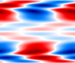
  $t_3$ in (b), the instantaneous structure of the corresponding mode is shown in figure 5.
Figure 5 shows the velocity components of several OTD modes at different instants of the pulsation cycle in the periodic regime, labelled according to the order of the eigenvalues of their steady counterparts. Mode  $u_1$ is reminiscent of the TS wave in steady Poiseuille flow that is modulated in the near-wall region, especially at the moment of maximum amplification (figure 5a). When the corresponding mode is most damped (figure 5b), the spatial structure is strongly affected by the pulsation close to the wall. Note that, since there is non-normal growth potential at all times, the most unstable direction will be a superposition of different modes, as can be seen in the region close to the centreline for mode $u_1$. Figure 5(c) shows one of the centre modes (mode $u_3$) that is very similar to its steady counterpart. Although the spatial structure is somewhat altered due to non-normality, the spatial structure of the OS mode is clearly visible and the growth rate is unaffected. Finally, figure 5(d) shows the spatial structure of mode $u_4$ when it is most amplified, resembling the second least stable mode of the T-branch of the OS spectrum.

Figure 5. Instantaneous  $u$ and $v$ components of $u_i$ at different times $t_j$ along the pulsation cycle in the periodic regime as marked in figure 4(b); (a) $u_1$ at maximum amplification ( $t_1 = 428$), (b) $u_1$ at maximum damping ( $t_2 = 473$), (c) $u_3$ at $t=t_1$, (d) $u_4$ at maximum amplification ( $t_3 = 432$). The parameters are the same as in figure 4(b). Videos of the evolution of $u_1$ and $u_4$ over the pulsation cycle are available in the supplementary material as Movie 1 and Movie 2 available at https://doi.org/10.1017/jfm.2021.743, respectively.
In order to characterise the different modes more precisely, it is instructive to consider also the phase speed i.e. the imaginary part of the eigenvalue since  $\alpha =1$. Combining the traces of the instantaneous real and imaginary parts of the eigenvalue in the periodic regime and comparing them for different values of $\tilde {Q}$ exhibits a clear pattern shown in figure 6 for the two dominant oscillating eigenvalues for $Wo= 10$ (a,b) and $Wo= 25$ (c,d). We observe that the eigenvalue excursions are more pronounced for large pulsation amplitudes, especially at low frequency, and are generally more erratic for higher pulsation frequencies. For $Wo=10$, low pulsation amplitudes lead mostly to a comparatively small variation of the growth rate at relatively constant phase speed and then abruptly begin with very large excursions of both growth rate and phase speed for amplitudes beyond $\tilde {Q}=0.1 - 0.15$. Nevertheless, as $\tilde {Q}$ approaches 0 (steady state), the periodic orbits contract around the most unstable eigenvalues of the A-branch, confirming the identification based on the spatial structure of the modes in figure 5. Comparing the eigenvalue orbits for the same pulsation frequency, we see that both oscillating modes exhibit similar trends throughout the tested amplitude range, with mode 4 being more stable throughout than mode 1, as in the steady case.

Figure 6. Periodic orbits in the complex plane of the instantaneous eigenvalues  $\lambda _1$ and $\lambda _4$ of $L_r$ for different pulsation amplitudes $\tilde {Q}$ at $\mbox {Re}=7500, \alpha =1, \beta = 0$ compared with the corresponding OS spectrum. The shaded area indicates linear instability. The rows correspond to the two different values of $Wo$ and every column corresponds to a different mode. For $Wo = 10$: $\lambda _1$ (a) and $\lambda _4$ (b). For $Wo = 25$: $\lambda _1$ (c) and $\lambda _4$ (d).
The two distinct behaviours of the modes in the pulsating case in comparison with the steady counterpart is linked to the spatial localisation of the modes in relation to the base flow modulation. The pulsations superimposed onto the parabolic profile exhibit the most variation close to the walls leading to the eigenvalue excursions of modes 1 and 4 that have similar behaviour. Close to the centreline of the channel, the pulsating velocity component is flat so that centre modes see very little variation of the base flow curvature in comparison with the steady case. Their growth rates are largely unaffected. It is a general feature that all modes on the A-branch of the OS spectrum are more strongly affected by the pulsations than the modes on the P-branch, especially the closer they are to the centreline.
Also in terms of the phase speed the eigenvalues have a much less erratic behaviour as the pulsation amplitude increases. While the phase speeds of all eigenvalues oscillate with the mean flow amplitude, only the eigenvalues from the A-branch noticeably deviate from a purely sinusoidal variation in phase speed. Towards the upper limit of the amplitude range ( $\tilde {Q} = 1.0$) and low frequencies, where we observe the largest excursions of the modulated eigenvalue traces, we also begin to see the pulsations slightly affect the growth rates of the centre modes. This is because, at these extreme amplitudes, the modifications of the local base flow profiles due to the pulsations are no longer confined to the near-wall regions. This effect is more pronounced for lower frequencies since the associated oscillating boundary layer is thicker and thus reaches further into the channel.
The periodic orbits give a good overview of the eigenvalue excursions in the complex plane but are ill suited to compare different eigenvalue traces at specific instants along the pulsation cycle since the time dependence is implicit. In this context, it is more useful to consider the intracyclic modulation of the real and imaginary parts of mode 1 (modulated TS wave) in the periodic regime separately over time to link the instability characteristics to flow features. The eigenvalue traces are shown in figure 7 at  $Wo=10$ 7(a,b) and $Wo=25$ 7(c,d) for the same values of $\tilde {Q}$ as in figure 6.

Figure 7. Intracyclic modulation of the most unstable eigenvalue ( $\lambda _1$) in the periodic regime for different pulsation amplitudes $\tilde {Q}$ at $\mbox {Re}=7500, \alpha =1, \beta = 0$. The horizontal dashed line indicates the leading eigenvalue of the corresponding OS spectrum; (a,b) $Wo=10$, (c,d) $Wo=25$.
Comparing the eigenvalue traces with the corresponding Floquet exponents (cf. figure 3), it is evident that the growth rates over the pulsation cycle are considerably larger than the net cycle-to-cycle growth rate. This becomes particularly clear when comparing them with the temporal growth rate of the corresponding steady case (dashed black line). The steady growth rate is of roughly the same order of magnitude as the leading Floquet exponent at moderate pulsation amplitudes which themselves are 1–2 orders of magnitude smaller than the peak growth and decay rates of even very low pulsation amplitudes ( $\tilde {Q}=0.05$). These large intracyclic growth rates that are sustained for a large fraction of the period lead to the well-documented large perturbation amplitudes during a pulsation cycle (Pier & Schmid Reference Pier and Schmid2017).
Furthermore, it can be noted that, while the growth and decay rates tend to increase with the pulsation amplitude for all values of  $Wo$, the peak growth rates saturate at around 0.11 and damping rates rarely exceed $-0.15$ when the pulsation amplitudes exceed values of roughly $\tilde {Q} = 0.5$. The maximum growth rates achievable with pulsations are therefore lower than the peak values exploiting transient growth mechanisms. Due to the fact that, unlike transient growth mechanisms that act over short time scales, the high intracyclic growth rates are maintained over long periods of time, they lead to higher energy growth overall. Since the extremal growth rates saturate, the continued variation of the Floquet exponents for higher pulsation amplitudes is mainly due to variations of the distribution of amplification and damping throughout the cycle.
Due to the large parameter space it is prohibitively expensive to give an exhaustive description of the effect of pulsation here and we will focus on two combinations  $(Wo,\tilde {Q})$, namely $(10,0.5)$ and $(25,0.5)$, to illustrate the range of possible intracyclic variation and show some typical features of the stability of pulsatile Poiseuille flow. The streamwise velocity component of the OTD mode corresponding to $\lambda _1$ for these cases is shown in figures 8(b)–8(a) and 9(b)–9(a), respectively, at selected instants during the pulsation cycle showcasing prominent features. The simulations for this section were run with $r=12$. We only show mode 1 since mode 4 shows very similar behaviour and the remaining modes are centre modes that exhibit little variation over the pulsation cycle.

Figure 8. Instantaneous streamwise velocity component of  $u_1$ at different instants over a pulsation cycle for $Wo=10$ and $\tilde {Q}=0.5$ in the periodic regime (a) compared with the base flow profiles, the location of inflection points and the boundary layer thickness (b) as well as the instantaneous growth rate of the mode (c). The velocity fields and base flow profiles are shown for $t/T_0 = 0.06, 0.15, 0.59, 0.75$ marked as $t_1, \ldots ,t_4$, respectively. The distinction between stable and unstable inflection points is as in figure 1. The computations were performed with $r=12$. A video of the evolution of $u_1$ over the pulsation cycle is available in the supplementary material as Movie 3.

Figure 9. Same as figure 8 but for  $Wo=25$ and $\tilde {Q}=0.5$. The velocity fields and base flow profiles are shown for $t/T_0 = 0.06, 0.56, 0.62, 0.68$ marked as $t_1, \ldots ,t_4$, respectively. A video of the evolution of $u_1$ over the pulsation cycle is available in the supplementary material as Movie 4.
6.1.3. Stability characteristics at low Womersley numbers
For low frequency pulsations ( $Wo = 10$) and low pulsation amplitudes, the growth rate variations increase in amplitude with $\tilde {Q}$. The phases of growth and decay happen at approximately the same time along the cycle, positive amplification rates existing in the range $t/T_0 \in [0.14, 0.6]$. As the pulsation amplitude is further increased, these phases start lagging behind, aligning with the appearance of backflow for large pulsation amplitudes. The amplification phase is well correlated with the existence of an unstable inflection point outside of the oscillating boundary layer and the snapshots of the modes during this phase (figure 8(a), $t_2$ to $t_4$) clearly show the localisation of the mode at the wall-normal height of the inflection points. In fact, as a second (stable) inflection point appears at the beginning of the acceleration phase, it is also followed by the mode ( $t_3$). The structure of the amplified mode is largely unchanged over the considered range of pulsation amplitudes. The damping phase initiates as the inflection points collide and vanish ( $t_4$). The observation that the mode follows the base flow inflection points only once they move out of the oscillating Stokes layer is likely linked to the fact that oscillating Stokes layers are known to have a stabilising effect on disturbances, decaying faster than in a quiescent fluid due to viscous dissipation (Davis Reference Davis1976). The fact that regions very close to the wall do not promote instability has also been linked to low values of the wall-normal velocity ( $v$) prevailing there that plays a key role in linear growth mechanisms (Obremski et al. Reference Obremski, Morkovin, Landahl, Wazzan and Okamura1969).
As  $\tilde {Q}$ is increased past approximately 0.1, oscillations of the eigenvalue start appearing during the damping phase. As the amplitude is further increased, these oscillations intensify and finally coalesce, leading to strong damping at the beginning of the cycle that abruptly transitions to amplification. Snapshots of the $u$-component of mode 1 contrasting the spatial structure during the damping and the beginning of the amplification phase after are shown in figure 8(a) from $t_1$ to $t_2$, respectively. Instead of TS-like structures close to the wall that are not visible at all, the mode consists of vortices located half-way between the wall and the centre of the channel that are strongly tilted in flow direction. Their structure is comparable to Orr waves that, once they have tilted with the base flow and can no longer extract energy from it, also exhibit similar decay rates. The shift towards the centre of the channel is also reflected in the phase speed that increases dramatically when the mechanism picked up by the mode changes. The oscillations prior to the coalescence are related to intermittent changes of the growth mechanism from TS-like structures to Orr-like structures and back before the Orr waves shown in figure 8(a) at $t_1$ become dominant throughout the damping phase.
An interesting note is that the appearance of the oscillations that herald the shift of the mode as well as the increase of the maximal damping coincide with the limit between the cruising and ballistic regimes identified by Pier & Schmid (Reference Pier and Schmid2017) in the saturated nonlinear regime. The latter is characterised by the complete disappearance of perturbations of the base flow over parts of the pulsation cycle. When damping is strongest, the leading OTD mode has negligible amplitude close to the wall. In fact, none of the leading 6 OTD modes pick up on TS-like structures close to the wall during the damping phase, indicating that these structures are even more damped. At these lower pulsation frequencies the pulsation period is considerably longer than the viscous time scale, giving the perturbations time to decay completely from the nonlinear amplitudes with the major energy supply from the linear mechanisms cut off. The effect is similar to the intermittent transition observed in direct numerical simulations of pulsating pipe flow by Xu & Avila (Reference Xu and Avila2018), in which turbulent puffs completely decay at low Womersley numbers.
6.1.4. Stability characteristics at high Womersley numbers
In comparison with the low frequency case that seems to fall into one of two categories of intracyclic behaviour, the variations of growth rate and phase speed are much more complicated at higher pulsation frequencies. This reflects on the intercyclic growth that is highly non-monotonic. The large changes in intracyclic behaviour for small changes in pulsation amplitude suggest that several competing mechanisms exist simultaneously.
Due to the higher frequency the oscillating boundary layer is very thin compared with the channel diameter and the phase lag between the boundary layer and the flow rate variation is more pronounced and leads to a more inflectional base flow profile. In fact, already for  $\tilde {Q}=0.35$ the base flow profile exhibits inflection points at all times. Figure 9(b) shows the location of inflection points at $\tilde {Q} = 0.5$. Due to the phase lag of the boundary layer, the amplification and decay phases are shifted compared with the lower pulsation frequencies. A similar shift in the timing of the maximum decay is seen as $\tilde {Q}$ is increased, but no oscillations in the eigenvalue can be observed. The shape of the dominant mode never completely changes as is observed in figure 8(a) from $t_1$ to $t_2$, but remains similar to distorted waves localised at the wall, as shown in figure 9(a).
Also here, the amplification phase is generally correlated with the existence of two inflection points outside of the Stokes layer and the modes localise on them. The abrupt beginning of the amplification phase is related to the emergence of the second inflection point outside of the oscillating boundary layer that leads to the breakup of the strongly sheared vortex ( $t_2$) into two separate vortices ( $t_3$), each localising on one of the inflection points. The phase of the two vortices quickly aligns as the growth rate peaks to reestablish a single near-wall wave ( $t_4$). The wall waves stay localised on the inflection points during the entire amplification phase. The beginning of the damping phase is again closely related with the collision and disappearance of the inflection points ( $t_1$). Although the fact that pulsation and viscous time scales are similar would suggest that local properties of the base flow profile play a less important role for the stability characteristics, we see that the existence of inflection points outside of the oscillating boundary layer is intimately linked to the amplification phases even at high pulsation frequencies.
6.1.5. Pulsations and non-normality
The linearised Navier–Stokes operator is highly non-normal, which can lead to considerable transient growth due to the non-orthogonality of its eigendirections. In order to analyse the impact of non-normality on the stability characteristics, we need a measure for the non-normal growth potential, i.e. the proportion of numerical abscissa  $\sigma _{max}$, including both modal and non-modal contributions, that cannot be explained by modal mechanisms alone. Since $\sigma _{max}$ always equals or exceeds the growth rate of the least stable eigenvalue $\lambda _1$, equality implying normality of the operator for which the non-normal growth potential is zero, we choose the difference $\sigma _{max}-\lambda _1$ as a measure for this potential (although other choices are possible). Obviously, the perturbations that will experience the growth rates given by $\sigma _{max}$ and $\lambda _1$, respectively, will not be the same in the non-normal case. Therefore, their difference is not a measure for the non-normal growth potential of a specific perturbation but instead a global indicator of the non-normal growth potential over all possible perturbations due to non-normality.
Comparing again figures 4(a) and 4(b), this time focusing on the numerical abscissa, we see that it follows the modulation of the oscillating eigenvalues. The non-normal growth potential is much less variable than the eigenvalues themselves and seems to change only little as the subspace size is doubled to  $r=12$, even though we observe both large variations of the intracyclic growth rates and highly damped Floquet exponents compared with the steady case (see figure 3). Moreover, the fact that the general structure of the eigenvectors does not change dramatically over the pulsation cycle makes an incidental correlation of $\sigma _{max}$ and $\lambda _i$ improbable. This might indicate that the numerical abscissa is already saturated with few OTD modes. This is in fact not the case, as can be seen in figure 10(a), showing the evolution of the numerical abscissa as the OTD subspace dimension is increased up to $r=100$.

Figure 10. Variation of the numerical abscissa  $\sigma _{max}$ of the reduced operator $L_r$ for different choices of $r$ at $Wo=25$ and $\tilde {Q}=0.2$ in the limit cycle. Blue to red: $r = 6, 12, 16, 20, 30, 40, 70, 100$ (a). The base flow acceleration/deceleration is indicated by the black line representing $Q(t)$ schematically (not to scale). (b) A close-up around the numerical abscissa of the corresponding OS spectrum (dashed line) and only the curves for $r=70,100$ are visible.
We observe that the maximum instantaneous growth in the subspace continues to increase as  $r$ is increased, only converging slowly as we reach $r=100$. It is known for plane Poiseuille flow that an accurate prediction of transient growth using an eigenmode expansion requires a large number of modes up to the S-branch, although these are highly damped (Reddy & Henningson Reference Reddy and Henningson1993). The present results indicate that this is true also when we look for transient growth potential within the instantaneously most unstable subspace in pulsating Poiseuille flow, i.e. that growth and decay due to the base flow pulsations do not exploit non-normality but instead coexist with it. This conclusion is in line with the observation that the maximum instantaneous growth rate in the pulsating flow case for $r=100$ is oscillating symmetrically within less than 1 % of the steady value (figure 10b). To cross-check, the maximum non-normal growth rate was computed for the steady case using 100 modes, matching with the value computed from the OS operator to within 0.17 % (not shown), proving that this subspace size is sufficient to capture almost the full non-normal growth potential. The results show that the small fluctuation of the numerical abscissa relative to the steady value over a pulsation cycle is nearly in phase with the acceleration/deceleration of the base flow measured by the sign of ${\textrm {d}}Q/{\textrm {d}}t$. Nevertheless, further studies are necessary to confirm that the growth indeed saturates and to analyse the behaviour for other frequencies and pulsation amplitudes.
The evidence shows that the pulsations mainly affect certain modal growth mechanisms (i.e. the exponential growth rates of the eigenvalues on the A-branch) without noticeably influencing the overall potential for non-normal growth compared with the steady case. To relate this result to earlier studies of optimal initial conditions for Poiseuille flow, these results practically mean that the known transient growth mechanisms in Poiseuille flow (e.g. the Orr mechanism for 2-D channel flow) are unaltered by the pulsations, i.e. the initial growth curves for these perturbations will look similar in both pulsating and steady cases. This does not mean, that there cannot be other transient phenomena that crucially rely on pulsations to emerge but these must be very different from the steady 2-D transient mechanisms, probably act over more than a pulsation period and are heavily restricted in terms of time scales if they are to be relevant compared with modal growth.
6.1.6. Subharmonic perturbation cycles
As we have seen in the previous sections, the variation of the instantaneous eigenvalues of the reduced operator  $L_r$ in the limit cycle are characterised either by convergence to the steady values in the case of centre modes or, in the case of eigenvalues from the A-branch, an alignment with the base pulsation frequency. While this is true for most eigenvalue traces, a third alternative exists for the evolution of the eigenvalues. It was found that when the subspace size is sufficiently large, two or more eigenvalue traces merge to form interlaced subharmonic eigenvalue traces. This phenomenon is exemplified in figure 11, showing the eigenvalue traces of $L_r$ over three consecutive pulsation cycles for the same parameters as in figure 10(a) with $r=40$ modes. Note that we use the term ‘subharmonic’ as a general term denoting periodicity with integer multiples of the base period $T_0$.

Figure 11. Traces of selected eigenvalues of  $L_r$ corresponding to the A-branch of the spectrum for $\mbox {Re}=7500$, $\alpha =1$, $\beta =0$, $Wo=25$ and $\tilde {Q} = 0.2$ with $r=40$ in the limit cycle. Evolution of the growth rate in time for three consecutive pulsation cycles (a) and orbits in the complex plane over a single pulsation cycle (b). The three eigenvalues that are subharmonic are highlighted in both panels showing their period is $T = 3T_0$. All other eigenvalue traces, including the centre modes (not shown) have the same period as the base flow ( $T_0$). The black dots in (b) show the corresponding OS spectrum for reference.
In this situation, the orbit of the dominant eigenvalue has merged with two other orbits and the three eigenvalues follow the same path staggered in time such that the instantaneous spectrum of the reduced operator is periodic with the base frequency. Note that the changes in the periodicity of the individual eigenvalue traces does not affect the intercyclic growth rates nor the instantaneous stability characteristics since the subharmonic eigenvalues simply exchange places from one pulsation cycle to the next. It is interesting to note that period tripling, as observed in this example, is not the only subharmonic that can appear and other combinations have been found for different parameter values, e.g. eigenvalue traces of period  $2T_0$. It is likely that such subharmonics are the norm, especially for higher pulsation amplitudes that lead to larger eigenvalue excursions overall.
A comparison of the eigenvalue traces in figures 4(a,b) and 11(a) indicates that the reason the subharmonic cycles are absent for smaller subspace sizes ( $r$) is the intense damping of the modes during a large part of the period. If a particular eigenvalue is too damped relative to the others it drops out of the subspace spanned by the OTD basis, which invariably follows the most unstable directions. In fact, the comparatively large fluctuations of the eigenvalue when it is most damped compared with the rest of the cycle suggest that there are more eigenvalue crossings with more damped modes. This could mean that an even larger subspace size is required to trace the full path of the dominant eigenvalue that might, in fact, cover more than just three periods when completely mapped.
A detailed analysis of the subharmonic orbits is outside of the scope of this work, not least because the accurate computation of highly damped eigenvalues leads to unwieldy requirements on wall-normal resolution. A more promising approach for the study of the subharmonic orbits is a fully spectral approach. These analyses can then also accurately trace the damped part of the eigenvalue orbits that are possibly underresolved in this work. While the resolution affects the details of the eigenvalue orbits, the existence of subharmonic perturbation cycles is a persistent feature of the flow case since the eigenvalue crossings that herald them lie in the upper part of the spectrum that is well resolved. In fact, the first 6 modes (i.e.  $r\leq 12$) are accurately computed, as can be seen from the match between the growth rates of the leading centre modes and the OS spectrum in figures 4(a,b) and 11(a).
7. Discussion and conclusion
The OTD modes are a recent method for constructing an orthonormal basis of a finite-dimensional subspace spanning and optimally following the instantaneously dominant directions of the tangent space in time along a reference trajectory proposed by Babaee & Sapsis (Reference Babaee and Sapsis2016). Apart from the modal stability characteristics, they also capture non-modal growth within the most unstable subspace around a given trajectory. In this work, the potential of the OTD framework for the linear stability analysis of time-dependent flows is explored.
The OTD framework has been implemented in the spectral element code Nek5000 and applied to pulsating Poiseuille flow, allowing for a rigorous validation against the large amount of data that are available for this canonical flow configuration and proof of the accuracy of the implementation. In particular, the results for the leading Floquet exponents from Pier & Schmid (Reference Pier and Schmid2017) were accurately reproduced and new results obtained for a larger range of pulsation amplitudes than previously reported. Using the framework, the instantaneous variation of the dominant OTD mode of linearly (Floquet) unstable two-dimensional pulsating Poiseuille flow was tracked in the limit cycle and related to the well-known OS modes. This procedure allows for clear characterisation of the stability mechanisms and their interaction that lead to the non-uniform effect of pulsations on the stability of pulsating Poiseuille flow.
In the following, we discuss the main findings of this work. The first point focuses on general considerations concerning the OTD framework and guidelines for its application, while the remaining points pertain to the linear stability characteristics of pulsating Poiseuille flow obtained using the OTD modes.
(i) The OTD modes will recover the  $r$-dimensional most unstable subspace of the tangent space. Unfortunately, a general rule for the choice of the subspace size $r$ is not available since it is highly dependent on the system and the goal of the stability analysis. The existing guidelines are either based on the unstable part of the full operator and its symmetric part, which is exhaustive but can be prohibitively large in many systems, or on heuristics. Once $r$ is chosen, care must be taken in the analysis of the OTD modes since the transient phase between initialisation and convergence of the OTD modes to the instantaneously most unstable directions of the tangent space lacks a precise physical meaning. Although the alignment is exponentially fast, the exact time it takes in practice is highly dependent on the system as well as the initial conditions. Once converged, however, the OTD modes depend only on the trajectory pointwise and are memoryless (Blanchard & Sapsis Reference Blanchard and Sapsis2019b).
The OTD modes capture both modal and non-modal instabilities within the OTD subspace. This does not imply that the full non-normal growth potential of the complete system is captured since non-normal growth mechanisms may, and often do, involve the interaction of one or more very stable directions that do not appear in finite OTD subspaces of practical size.
The OTD framework can be used to compute reduced-order FTLEs along the trajectory and using the Blanchard & Sapsis formulation makes their computation particularly efficient at negligible extra cost (Babaee et al. Reference Babaee, Farazmand, Haller and Sapsis2017; Blanchard & Sapsis Reference Blanchard and Sapsis2019a). When considering time-periodic flows, it consequently yields the Floquet exponents with the practical advantage over classical Floquet methods that the framework can be applied directly to the unsteady problem requiring very little extra machinery beyond the standard routines for the solution of the base flow and the linearised Navier–Stokes operator. Moreover, the fact that the OTD modes capture the instantaneously dominant directions in phase space opens many opportunities for reduced-order modelling and control.
When applied to steady base flows, the OTD modes can be readily analysed and completely understood with the existing framework of linear stability analysis. It is therefore in the realm of unsteady flows, in particular flows exhibiting spatio-temporal variation of the base flow that the strengths of the OTD framework are most salient since these flows are inaccessible to global mode analysis. Examples of such flow cases include the analysis of streak instability in bypass transition (Andersson et al. Reference Andersson, Brandt, Bottaro and Henningson2001), chaotic edge states (Duguet, Willis & Kerswell Reference Duguet, Willis and Kerswell2008; Beneitez et al. Reference Beneitez, Duguet, Schlatter and Henningson2019) or the minimal seed of turbulence (Pringle & Kerswell Reference Pringle and Kerswell2010; Duguet et al. Reference Duguet, Monokrousos, Brandt and Henningson2013; Vavaliaris, Beneitez & Henningson Reference Vavaliaris, Beneitez and Henningson2020) or fully non-autonomous flows dictated by time-dependent external forcing or boundary conditions. While the OTD modes have shown to be successful in a statistical framework (Farazmand & Sapsis Reference Farazmand and Sapsis2016) or for flow control (Blanchard et al. Reference Blanchard, Mowlavi and Sapsis2018), most applications only use them as a stable numerical tool since the physical interpretation of a particular instance of the instantaneous OTD modes on top of a fully transient, nonlinear base flow is far from trivial but might be the key to the analysis of non-autonomous flow cases.
(ii) The OTD framework applied to pulsating Poiseuille flow in the periodic regime generates modes that correspond to the pulsating equivalent of the OS modes. The amount of modulation these modes experience is determined by their spatial localisation in the channel. The wall modes of the A-branch, including the ubiquitous TS waves, are strongly modulated over the pulsation cycle by the changes in the base flow profile close to the oscillating Stokes layer and exhibit considerable fluctuations in both exponential growth rate and phase speed. On the other hand, the growth rates of the modes of the P-branch or centre modes are largely unaffected by the pulsation. It is only for extreme pulsation amplitudes at low frequency that the base flow modulation reaches the centreline, inducing a noticeable intracyclic variation in the leading centre modes.
(iii) The base flow profiles for pulsating Poiseuille flow are highly inflectional and it was found that the amplification phase of the pulsation cycle is well correlated with the existence of two inflection points of the base flow profile outside of the oscillating Stokes layer close to the wall. This result was consistent over the entire range of Womersley number considered. The transition from amplification to damping is generally linked to the collision and disappearance of these inflection points. For low frequencies, where the base flow profile is much less inflectional, the amplification begins already as the first inflection point moves out of the boundary layer. Intuitively, the amplification phase is associated with a W- or  $\varLambda$-shaped base flow profile that exhibits two separate shear layers and low flow rates while perturbations decay when the bulk flow is forward.
(iv) The leading OTD mode generally has the structure of a travelling wave close to the wall, similar to the TS waves in steady flow for most of the pulsation cycle. The eigenfunctions are localised in the wall-normal direction at the height of the inflection points in the base flow profile, in particular during the amplification phase. This is in line with the nonlinear simulations of Pier & Schmid (Reference Pier and Schmid2017) that observe the modulated exponential growth of similar instability waves. As the pulsation amplitude is increased, the vortices are heavily sheared by the mean flow but generally maintain their spatial structure and stay localised close to the wall indicating that, while modulated by the pulsation, the basic mechanism governing the stability is preserved over most of the parameter range. This behaviour prevails also in regions of the parameter space that are Floquet stable.
The only exception to this rule is found during the damping phase for low pulsation frequencies and pulsation amplitudes beyond approximately  $\tilde {Q}=0.1$. For these configurations, the strongly damped leading mode moves away from the wall entirely and its spatial structure resembles that of decaying Orr waves that lean with the mean shear. The corresponding nonlinear simulations by Pier & Schmid (Reference Pier and Schmid2017) also exhibit a different behaviour in this parameter range, termed the ‘ballistic regime’, in which the perturbations completely vanish over part of the pulsation cycle. Considering that characteristic TS-like instabilities were not found in the six-dimensional most unstable subspace during this phase, indicating that they are very damped, it is likely that the change of linear instability mechanism is intimately linked to the appearance of the ballistic regime. This view is supported by the fact that, for the parameter choices investigated, the modulated TS waves (as well as similar wall structures from the A branch) are the only modes that are unstable during the pulsation cycle so that, during their decay phase, there are no linear growth mechanisms available to the flow. At the same time, TS-like structures similar to the saturated nonlinear waves are heavily damped over a long period of time due to the low pulsation frequency, which could explain their complete disappearance and the fact that no other perturbations are excited during part of the oscillation cycle. Direct numerical simulations of pulsating pipe flow by Xu & Avila (Reference Xu and Avila2018) show full relaminarisation of turbulent puffs at low pulsation amplitudes that may hinge on a similar mechanism.
(v) By increasing the size of the OTD subspace considerably to  $r=100$ for a specific case in order to capture the full non-normal growth potential, it was shown that the pulsations have little effect on the non-normality of the operator compared with the steady case. The intracyclic variations of the numerical abscissa for a moderate pulsation amplitude ( $\tilde {Q}=0.2$) were found to lie within 1 % of the steady value. This result indicates that the changes in the instability characteristics due to pulsation do not rely on non-normality but are instead due to the modulation of modal mechanisms that coexist independently. This result would suggest that, while large transient growth responses can be obtained from an optimal initial condition for pulsating flows as shown by Xu et al. (Reference Xu, Song and Avila2021) and Tsigklifis & Lucey (Reference Tsigklifis and Lucey2017) in similar geometries, it is likely difficult for the transient mechanisms to fuel their growth efficiently using the base flow pulsations.
(vi) For small and moderate subspace sizes, all OTD modes are periodic with the base flow pulsation frequency in the limit cycle. When the subspace is large enough, the orbit of the dominant eigenvalue of the reduced operator merges with more damped orbits to create subharmonic oscillations that have not been documented for pulsating Poiseuille flow before. They indicate that the perturbations have a more intricate behaviour than previously assumed and that a restriction to perturbations at the base frequency will hide relevant subharmonic structures. The appearance of the subharmonic orbits is likely linked to the transient proximity of the eigenvalues in the complex plane during the pulsation cycle, leading them to switch place. On the other hand, a bifurcation cascade that is one of the routes to chaos (Feigenbaum Reference Feigenbaum1980) is unlikely their cause since the subharmonic orbits do not exhibit the characteristic period doubling and do not seem to emerge at an accelerating rate. Further research is necessary to analyse and understand the appearance and behaviour of the subharmonic perturbation cycles. Given that the dominant eigenvalues are very damped during part of the subharmonic cycle, such an endeavour will need to have a high wall-normal resolution and should therefore be carried out with a spectral approach.
It may be noted that, irrespective of whether a spectral or pseudo-spectral method is employed for the study of perturbations on a periodic base flow, the OTD framework is ideally suited for the task because it allows the perturbations to be followed even if they are highly damped without assumptions about their temporal periodicity.
To highlight the physical insights gained from applying the OTD framework to the case of pulsating Poiseuille flow, we summarise the main aspects of the discussion.
The main driver of instability in pulsating Poiseuille flow just beyond to the critical Reynolds number for linear instability is a modulated version of the TS wave known from steady shear flows that is prominent across the parameter space considered in this work. This result is in qualitative agreement with DNS results in the literature. Moreover, at low pulsation frequencies, the damping phase is associated with a different spatial structure reminiscent of Orr waves leaning with the mean shear and the disappearance of perturbations akin to TS waves which may explain the emergence of the ballistic regime in nonlinear simulations by Pier & Schmid (Reference Pier and Schmid2017). The amplification phase is marked by the co-existence of two inflection points in the base flow profile outside of the boundary layer. In all cases damping begins close to the collision and disappearance of the inflection points closest to the centreline. For low pulsation frequencies, where the base flow profile only has a single inflection point for most of the cycle, the amplification begins when it moves out of the boundary layer. The dominant perturbations are shown to localise at the inflection points, highlighting their importance even in transient flow stability at high pulsation frequencies. The computations spanning almost the full non-normal growth potential of the linear operator indicate that pulsations have little effect on known 2-D transient growth mechanisms such as the Orr mechanism. Finally, as the size of the OTD subspace was increased considerably, some of the eigenvalue orbits were seen to merge into subharmonic cycles. This interesting phenomenon is not yet fully understood but is likely crucial for a complete picture of the transient stability of pulsating Poiseuille flow.
Supplementary movies
Supplementary movies are available at https://doi.org/10.1017/jfm.2021.743.
Acknowledgements
The authors thank Y. Duguet for helpful discussions on the OTD modes and gratefully acknowledge the help of B. Pier who made his precise computations of the linear temporal growth rates for pulsating Poiseuille flow available for validation. The insightful discussions with P. Negi in the initial implementation process in Nek5000 are greatly appreciated by J.S.K. and M.B. thanks P. Schlatter for the stimulating discussions. The authors also thank the reviewers for helpful comments that considerably improved the quality of the paper.
Funding
Financial support for this work was provided by the European Research Council under grant agreement 694452-TRANSEP-ERC-2015-AdG and by the Swedish Research Council (VR) grant no. 2016-03541. The computations were performed on resources by the Swedish National Infrastructure for Computing (SNIC) at the PDC Center for High Performance Computing at the Royal Institute of Technology (KTH).
Declaration of interests
The authors report no conflict of interest.
Appendix A. Numerical integration in Nek5000 and validation
A.1. Computing the OTD forcing
As we have seen in (3.4), the evolution equation for the OTD basis vectors is very similar to the standard linearised Navier–Stokes system and the OTD solver can therefore be built by adding an appropriate forcing term using the reduced operator constructed by combining the existing routines from the linear solver. Nek5000, like most modern high-performance computational fluid dynamics (CFD) codes, relies on a matrix-free method to integrate the Navier–Stokes equation that avoids the explicit computation of the linear operator, instead constructing the action of the operator on the current state. In order to construct the necessary forcing term to adapt the standard linearised Navier–Stokes solver to integrate the OTD evolution equation, we therefore need to isolate the action of the linearised operator on the perturbation field itself, before boundary conditions and external forcing are applied. In this process, it is paramount to ensure accuracy with over-integration using the 3/2 rule to avoid introducing spurious modes into the operator when computing the nonlinear terms.
A.2. Initial conditions and boundary conditions
The OTD modes are perturbations to a reference flow trajectory. Close to solid walls the OTD modes are subject to the same no-slip condition as the base flow. For the in- and outflow boundaries homogeneous Dirichlet or periodic conditions are imposed in our case for the single and multisession set-ups, respectively (see § A.4 for details about the multisession set-up).
The OTD framework requires the initial conditions for the OTD basis to be orthonormal and to satisfy the boundary conditions of the problem. In Nek5000 it is particularly simple to achieve this for any initial condition since the solution technique is based on the Helmholtz–Hodge decomposition during which the initial condition is projected onto the closest divergence-free space. After the first timestep, the fields are therefore automatically solenoidal and satisfy the boundary conditions. After orthonormalisation, in our case performed using the modified Gram–Schmidt (MGS) algorithm, also the orthonormality condition is satisfied.
A.3. Numerical loss of orthonormality of the basis vectors during numerical integration
The evolution equation for the OTD basis vectors (2.4) is derived under the constraint of orthonormality and it was shown that if the OTD basis is initially orthonormal, it will remain orthonormal for all times if  $\varPhi =-\varPhi ^{\textrm {T}}$ (Babaee & Sapsis Reference Babaee and Sapsis2016).
Regarding the numerical implementation of the method, the first remark to make is that the above statement is true only in the continuous sense; when integrating the OTD basis using finite precision arithmetic, the orthonormality constraint is no longer automatically satisfied since the unit norm constraint on the basis vectors is not enforced explicitly. Therefore, maintaining the orthogonality of the basis vectors is unachievable in practice. Small truncation errors suffice to cause a gradual loss of orthonormality of the OTD basis during the projection steps that, if unabated, will eventually lead to their collapse onto the most unstable direction in phase space. The conclusions are the same as those drawn in Wiesel (Reference Wiesel1993) for a similar algorithm to compute the Gram–Schmidt vectors. It is therefore necessary to periodically reorthonormalise the basis vectors, in particular before the eigendecomposition of the reduced operator is computed.
In the light of the equivalence between the OTD basis and continuously orthogonalised Gram–Schmidt vectors, we stress that this discussion is independent of the particular choice of internal rotation but instead stems from the fact that numerical implementations use finite precision arithmetic and the nonlinear forcing terms are evaluated explicitly. Any such implementation will therefore suffer from loss of orthonormality by the same process described above. Moreover, when comparing the OTD framework to the standard approach to generate Gram–Schmidt vectors, which is to advance the linear dynamics without forcing and then apply a Gram–Schmidt process to maintain orthonormality, it should be noted that incorporating the orthonormality condition into the evolution equation directly leads to an intrinsically more stable algorithm in the sense that departure from orthonormality, although inevitable, is slow compared with the unforced dynamics. The OTD framework therefore offers possibilities for case-specific optimisation to considerably increase the interval between reorthonormalisations which would make simulations less expensive overall, thus warranting the additional implementation effort required for the forcing terms.
In principle, the OTD basis can always be reorthonormalised at any given time to recover the accurate reduced operator but if implicit multistep timesteppers are being used, the solution is liable to diverge in subsequent timesteps if the basis is far from orthonormal and the orthonormalisation is not carried out over all timesteps in the stencil.
The cost of reorthonormalisation for different basis sizes from  $r=1$ to $r=32$ is shown in figure 12, plotting both the average absolute time for complete reorthonormalisation as well as the proportional cost per timestep. The simulations are otherwise identical and run on 2 cores to reach optimal scaling of the underlying code. From the data we see the typical quadratic increase of the cost of orthonormalisation as the basis size increases. Comparing the cost of reorthonormalisation with the rest of the timestep in the code used in this work, it proves to be a comparatively cheap operation if the OTD basis is of small or moderate size ( $r\leq 16$), incurring at most a computational overhead of 2 %. Consequently, we have chosen to increase the frequency of reorthonormalisation to have a safety margin. In fact, it can be expected that the reorthonormalisation cost can be further reduced with the use of optimised algorithms.

Figure 12. Computational cost of the Gram–Schmidt orthonormalisation per timestep using a simple modified Gram–Schmidt algorithm where  $t_s$ is the total time per timestep. All data points are averaged over 1000 timesteps with orthonormalisation at every step.
We note that these results are valid only for Nek5000. In other codes, the cost of reorthonormalisation may be considerably higher, especially for those working in transformed space since the inner products need to be performed in physical space and the transformations can be expensive e.g. if they require a fast Fourier transform (FFT). In these cases, it might be advantageous to further study the implications of reducing the number of reorthonormalisation steps to a minimum.
A.4. Spatially localised OTD modes
The standard procedure described above allows for the computation of the OTD subspace on the same physical domain as the reference trajectory. Such a global approach might have important drawbacks when it comes to the practical application of the framework, especially in large transient configurations with spatial inhomogeneity. The global nature of the minimisation strategy will identify the most salient instabilities in the whole flow field, which might be desirable when considering cases such as the jet in cross-flow where a global instability governs the flow dynamics and these structures are the object of study (Bagheri et al. Reference Bagheri, Schlatter, Schmid and Henningson2009b; Babaee & Sapsis Reference Babaee and Sapsis2016; Chauvat et al. Reference Chauvat, Peplinski, Henningson and Hanifi2020).
In more subtle scenarios, where a more detailed analysis of the spatial distribution and evolution of specific instabilities is of interest but these instabilities may not be the most prominent ones, the consideration of the full physical domain is prohibitive and might highlight other instability regions than those of interest. Typical examples are transitional flows at higher Reynolds numbers where the interesting dynamics in the boundary layers is easily shadowed by the strong instabilities in the turbulent region of the flow. Furthermore, if the accurate computation of the base flow requires a large domain to exclude boundary effects, a considerable part of the computational effort in the linear solves is used in the far field if the OTD modes are computed on the full domain. This is particularly inefficient if the region of interest for the stability calculation has a small spatial extent in comparison with the full domain.
The natural solution to this problem is to topologically separate the base flow and OTD subspace computations onto two overlapping grids with a one-way coupling from the base flow computation to the linear solver. A similar approach was used in Blanchard & Sapsis (Reference Blanchard and Sapsis2019c) in order to construct a localised controller using the OTD framework. While this task is trivial for steady base flows where the two simulations can be executed sequentially, the implementation using two simultaneous sessions for the OTD subspace and base flow computations respectively is more challenging. Although the base flow and perturbation fields can, in principle, be computed sequentially also in the transient case, a simultaneous implementation was chosen because the storage requirements for a sequential approach quickly become unwieldy. Note that each session can be executed on multi-core systems irrespective of the chosen set-up.
In this work, the separation of the two coupled simulations is implemented based on the overlapping grid method, dubbed ‘NekNek’, recently developed by Merrill et al. (Reference Merrill, Peet, Fischer and Lottes2016) that uses spectral interpolation to transfer data between the grids and maintains the third-order temporal accuracy of the single session implementation. In contrast to the original implementation of the method that is aimed at solving a single problem on partially overlapping grids to simplify the meshing process and improve local resolution, the present work separates the base flow computation from the perturbation problem.
The linear solver needs the full base flow solution and therefore requires the perturbation problem to be defined on a subdomain of the base flow domain for accurate interpolation. This interpolation step can be a performance bottleneck. Therefore, when the flow case allows it, the most expensive part of the interpolation, i.e. the set-up step in which the elements containing the interpolation points need to be identified in both meshes, is only run once at the beginning of the simulation.
A schematic flow chart of the computational structure of one timestep in the multisession set-up is shown in figure 13. The first session (left) computes the base flow on the full domain. The second session (right) receives the base flow information from the first session (via the interpolation step) and solves the  $r$ linear problems for the OTD basis vectors sequentially. Since the two sessions are fully independent of each other, with the exception of the interpolation, they only need to be synchronised once per timestep and the distribution of the jobs across the available MPI ranks can be easily optimised so as to ensure that the expensive computation (typically M1) never has to wait for the cheaper computation thus using the computational resources as efficiently as possible. This set-up allows not only for geometric flexibility in the mesh generation but also independent choices of polynomial order in each session as well as the possibility to accommodate various OTD space sizes while maintaining efficiency.

Figure 13. Flow chart showing the structure of the multisession set-up for one timestep. In a typical production set-up  $n \ll N$ and the available cores are distributed on the two sessions such that $O(N) \leq r \times O(n)$ is roughly satisfied over large parts of the computation, where $O$ is shorthand for the computational time to solution.
The dramatic reduction in the computational cost using the localised OTD modes can be appreciated for the computation of the flow around an airfoil with the stability analysis restricted to a small region around the leading edge of the airfoil. In a 2-D configuration, the cost of one additional OTD mode can easily drop to 5 % compared with the base flow computation (a reduction by a factor 20), the main bottleneck being the distribution of the available cores on the two sessions. For a 3-D simulation the gains in computational effort compared with a single session set-up are even more pronounced.
A.5. Boundary conditions for the localised problem
Localising the linear problem highlights the importance of choosing appropriate boundary conditions. It is well known that eigenvalue spectra are sensitive to simulation details, such as the boundary conditions, but also other numerical parameters such as grid spacing and box size (Chauvat et al. Reference Chauvat, Peplinski, Henningson and Hanifi2020). The implications are not as severe for the OTD method as might seem at first glance since the dominant modes typically show the least sensitivity to the numerical parameters. The purpose of the OTD method is to converge to the subspace that spans the most unstable directions and we can therefore expect the eigenvalues of the reduced operator  $L_r$ to be comparatively robust with regard to the details of the numerical implementation. Blanchard & Sapsis (Reference Blanchard and Sapsis2019c) come to similar conclusions with regard to the boundary conditions of the localised problem. Therefore, unless periodicity or no-slip conditions apply, Dirichlet conditions are set at the boundaries of the linear domain. In more complex scenarios, one needs to be careful with the choice of boundary conditions to avoid possible numerical artefacts such as reflections at the outflow.
A.6. Numerical set-up for multisession runs
In the multisession set-up, two fully separate simulations are run simultaneously. The two meshes used are shown superimposed in figure 14 showing that the domain on which the perturbations are computed (red) is a subset of the base flow domain (black). The base flow mesh is much coarser than the mesh for the linear solves since the resolution issues mentioned above do not occur when solving the base flow. The polynomial order for the base flow computation is set to  $N=7$ that is sufficient to accurately resolve the base flow profile while the perturbation session has a polynomial order of $N=9$ as in the single session set-up. All other settings such as solver tolerances and timestep size are identical to the single session runs. The boundary conditions for the perturbations are identical to the single session runs.

Figure 14. Two-dimensional spectral element meshes for the multisession set-up. The base flow is computed on mesh M1 (black) and the perturbations on mesh M2 (red). The boundary conditions are identical to the single session runs (not shown, cf. figure 2).
For plane Poiseuille flow the base flow is known analytically. Nevertheless, to feature the multisession set-up, it is computed explicitly alongside the perturbations for illustrative purposes. For the base flow computation, apart from the no-slip condition on the walls, the pressure gradient  ${\rm \Delta} p = -G_x^{(0)}$ is imposed in streamwise direction as a constant volumetric forcing term. In the more general setting of complex and time-dependent problems, there is usually no alternative to computing the base flow trajectory in real time alongside the linearised problem.
The plane Poiseuille flow case that we compare with Babaee & Sapsis (Reference Babaee and Sapsis2016) is initialised with the same optimal initial conditions as in the reference, i.e. the initial condition for optimal growth at  $T_{max}=25.06$ for $\mbox {Re}=5000$ and $(\alpha ,\beta )=(1,1)$.
A.7. Validation for 3-D plane Poiseuille flow
In general, a computation of the OTD subspace using a complex OS/SQ solver in Fourier space (similar to the approach chosen in Babaee & Sapsis Reference Babaee and Sapsis2016) and using a code in physical space as Nek5000 cannot be expected to yield the same results. In the particular case of the optimal initial conditions for maximum growth at  $T_{max}=25.06$ for $\mbox {Re}=5000$ and $(\alpha ,\beta )=(1,1)$, the optimal and first suboptimal are purely real (and hence also orthogonal in physical space) and the most unstable directions remain real as they evolve towards the least stable eigendirections of the OS/SQ operator. Therefore, the complex OS/SQ solver and Nek5000 in physical space compute identical OTD subspaces for $r=2$ and can be compared directly. Figure 15(a) shows the comparison between the eigenvalue traces computes with Nek5000 with data from Babaee & Sapsis (Reference Babaee and Sapsis2016). The data are in very good agreement overall considering the high sensitivity of the exact temporal evolution of growth rates on numerical implementation details. Note that the numerical abscissa coincides with the least stable eigenvalue for all time since the modes are orthogonal and hence no non-normal growth is possible within the subspace they span.

Figure 15. Instantaneous real eigenvalues and numerical abscissa of the reduced operator  $L_r$ for 3-D plane Poiseuille flow at $\mbox {Re}=5000$, $(\alpha ,\beta )=(1,1)$. (a) Comparison of the values computed with Nek5000 (solid lines, index 1) and data extracted from Babaee & Sapsis (Reference Babaee and Sapsis2016) for the numerical abscissa and the subdominant eigenvalue (crosses, ref) for $r=2$. (b) Comparison of the data computed with Nek5000 using the single session (solid lines, index 1) and multisession (circles, index 2) set-ups for $r=3$. The dashed lines indicate the corresponding OS/SQ spectrum.
The second suboptimal for this configuration is not orthogonal to the two previous (sub)optima in physical space and the temporal evolution of the eigenvalues will be different between real and complex implementations. Figure 15(b) shows the same configuration as figure 15(a) but using 3 modes computed with Nek5000 (solid lines). This figure can be compared with figure 5 in Babaee & Sapsis (Reference Babaee and Sapsis2016) to appreciate the differences. The symbols indicate the results of a multisession run for the same configuration that matches the single session data perfectly, showing that the separation of base flow and perturbation computations does not affect the accuracy of the stability calculations.


 Open access