


1. Introduction
Static analysis tools based on abstract interpretation are complicated software systems. They are complicated due to the complications of programming language semantics and the subtle invariants required to achieve meaningful results. They are also complicated when dedicated analysis algorithms are required to deal with certain types of properties, for example, one algorithm for inferring points-to information and another for checking array-out-of-bounds accesses. Thus, static analysis tools themselves are subject to subtle programming errors. From a software engineering perspective, it is therefore meaningful to separate the specification of the analysis as much as possible from the algorithm solving the analysis problem for a given program. In order to be widely applicable, this algorithm therefore should be as generic as possible.
In abstract interpretation-based static analysis, the analysis of a program, notably an imperative or object-oriented program, can naturally be compiled into a system of abstract equations. The unknowns represent places where invariants regarding the reaching program states are desired. Such unknowns could be, for example, plain program points or, in case of interprocedural analysis, program points together with abstract calling contexts. The sets of possible abstract values for these unknowns then correspond to classes of possible invariants and typically form complete lattices. Since for infinite complete lattices of abstract values the number of calling contexts is also possibly infinite, interprocedural analysis has generally to deal with infinite systems of equations. It turns out, however, that in this particular application, only the values of those unknowns are of interest that directly or indirectly influence some initial unknown. Here, local solving comes as a rescue: a local solver can be started with one initial unknown of interest. It then explores only those unknowns whose values contribute to the value of this initial unknown.
One such generic local solver is the top-down solver TD (Charlier and Van Hentenryck Reference Charlier and Van Hentenryck1992; Muthukumar and Hermenegildo Reference Muthukumar and Hermenegildo1990). Originally, the TD solver has been conceived for goal-directed static analysis of Prolog programs (Hermenegildo and Muthukumar Reference Hermenegildo and Muthukumar1989; Hermenegildo and Muthukumar Reference Hermenegildo and Muthukumar1992) while some basic ideas can be traced back to Bruynooghe et al. (Reference Bruynooghe, Janssens, Callebaut and Demoen1987). The same technology as developed for Prolog later turned out to be useful for imperative programs as well (Hermenegildo Reference Hermenegildo2000) and also was applied to other languages via translation to CLP programs (Gallagher and Henriksen Reference Gallagher and Henriksen2006; Hermenegildo et al. Reference Hermenegildo, Mendez-Lojo and Navas2007). A variant of it is still at the heart of the program analysis system Ciao (Hermenegildo et al. Reference Hermenegildo, Bueno, Carro, LÓpez-GarcÍa, Mera, Morales and Puebla2012; Hermenegildo et al. Reference Hermenegildo, Puebla, Bueno and LÓpez-GarcÍa2005). The TD solver is interesting in that it completely abandons specific data structures such as work-lists, but solely relies on recursive evaluation of (right-hand sides of) unknowns.
Subsequently, the idea of using generic local solvers has also been adopted for the design and implementation of the static analysis tool Goblint (Vojdani et al. Reference Vojdani, Apinis, RÕtov, Seidl, Vene and Vogler2016) – now targeted at the abstract interpretation of multi-threaded C. Since the precise analysis of programming languages requires to employ abstract domains with possibly infinite ascending or descending chains, the solvers provided by Goblint were extended with support for widening as well as narrowing (Amato et al. Reference Amato, Scozzari, Seidl, Apinis and Vojdani2016). Recall that widening and narrowing operators have been introduced in Cousot and Cousot (Reference Cousot, Cousot, Graham, Harrison and Sethi1977); Cousot and Cousot (Reference Cousot and Cousot1992) as an iteration strategy for solving finite systems of equations: in a first phase, an upward Kleene fixpoint iteration is accelerated to obtain some post-solution, which then, in a second phase, is improved by an accelerated downward iteration. This strict separation into phases is given up by the algorithms from Amato et al. (Reference Amato, Scozzari, Seidl, Apinis and Vojdani2016). Instead, the ascending iteration on one unknown is possibly intertwined with the descending iteration on another. The idea is to avoid unnecessary loss of precision by starting an improving iteration on an unknown as soon as an over-approximation of the least solution for this unknown has been reached. On the downside, the solvers developed in Amato et al. (Reference Amato, Scozzari, Seidl, Apinis and Vojdani2016) are only guaranteed to terminate for monotonic systems of equations. Systems for interprocedural analysis, however, are not necessarily monotonic. The problems concerning termination as encountered by the non-standard local iteration strategy from Amato et al. (Reference Amato, Scozzari, Seidl, Apinis and Vojdani2016) were resolved in Frielinghaus et al. (Reference Frielinghaus, Seidl and Vogler2016) where the switch from a widening to a narrowing iteration for an unknown was carefully redesigned.
When reviewing advantages and disadvantages of local generic solvers for Goblint, we observed in Apinis et al. (Reference Apinis, Seidl, Vojdani, Probst, Hankin and Hansen2016) that the extension with widening and narrowing from Amato et al. (Reference Amato, Scozzari, Seidl, Apinis and Vojdani2016) could nicely be applied to the solver TD as well – it was left open, though, how termination can be enforced not only for monotonic, but for arbitrary systems of equations. In this paper, we settle this issue and present a variant of the TD solver with widening and narrowing which is guaranteed to terminate for all systems of equations – whenever only finitely many unknowns are encountered.
Besides termination, another obstacle for the practical application of static analysis is the excessive space consumption incurred by storing abstract values for all encountered unknowns. Storing all these values allows interprocedural static analysis tools like Goblint only to scale to medium-sized programs of about 100k LOC. This is in stark contrast to the tool AstrÉe, which – while also being implemented in OCaml – succeeds in analyzing much larger input programs (Cousot et al. Reference Cousot, Cousot, Feret, Mauborgne, MinÉ and Rival2009). One reason is that AstrÉe only keeps the abstract values of a subset of unknowns in memory, which is sufficient for proceeding with the current fixpoint iteration. As our second contribution, we therefore show how to realize a space-efficient iteration strategy within the framework of generic local solvers. Unlike AstrÉe which iterates over the syntax, generic local solvers are application-independent. They operate on systems of equations – no matter where these are extracted from. As right-hand sides of equations are treated as black boxes, inspection of the syntax of the input program is out of reach. Since for local solvers the set of unknowns to be considered is only determined during the solving iteration, also the subset of unknowns sufficient for reconstructing the analysis result must be identified on the fly. Our idea for that purpose is to instrument the solver to observe when the value of an unknown is queried, for which an iteration is already on the way. For equation systems corresponding to standard control-flow graphs, these unknowns correspond to the loop heads and are therefore ideal candidates for widening and narrowing to be applied. That observation was already exploited in Apinis et al. (Reference Apinis, Seidl, Vojdani, Probst, Hankin and Hansen2016) to identify a set of unknowns where widening and narrowing should be applied. The values of these unknowns also suffice for reconstructing the values of all remaining unknowns without further iteration. Finally, we present an extension of the TD solver with side effects. Side effects during solving means that, while evaluating the right-hand side for some unknown, contributions to other unknowns may be triggered. This extension allows to nicely formulate partial context-sensitivity at procedure calls and also to combine flow-insensitive analysis, for example, of global data, with context-sensitive analysis of the local program state (Apinis et al. Reference Apinis, Seidl, Vojdani and Igarashi2012). The presented solvers have been implemented as part of Goblint, a static analysis framework written in OCaml.
This paper is organized as follows: First, we recall the basics of abstract interpretation. In Section 2, we show how the concrete semantics of a program can be defined using a system of equations with monotonic right-hand sides. In Section 3, we describe how abstract equation systems can be used to compute sound approximations of the collecting semantics. Since the sets of unknowns of concrete and abstract systems of equations may differ, we argue that soundness can only be proven relative to a description relation between concrete and abstract unknowns. We also recall the concepts of widening and narrowing and indicate in which sense these can be used to effectively solve abstract systems of equations. In Section 4, we present the generic local solver
 $\mathbf{TD}_{\mathbf{term}}$
. In Section 5, we show that it is guaranteed to terminate even for abstract equation systems with non-monotonic right-hand sides. In Section 6, we prove that it will always compute a solution that is a sound description of the least solution of the corresponding concrete system. In Section 7, we present the solver
$\mathbf{TD}_{\mathbf{term}}$
. In Section 5, we show that it is guaranteed to terminate even for abstract equation systems with non-monotonic right-hand sides. In Section 6, we prove that it will always compute a solution that is a sound description of the least solution of the corresponding concrete system. In Section 7, we present the solver
 $\mathbf{TD}_{\mathbf{space}}$
, a space-efficient variation of
$\mathbf{TD}_{\mathbf{space}}$
, a space-efficient variation of
 $\mathbf{TD}_{\mathbf{term}}$
that only keeps values at widening points. In Section 8, we prove that it terminates and similar to
$\mathbf{TD}_{\mathbf{term}}$
that only keeps values at widening points. In Section 8, we prove that it terminates and similar to
 $\mathbf{TD}_{\mathbf{term}}$
computes a sound description of the least solution of the corresponding concrete system. In Section 9, we introduce side-effecting systems of equations, and the solver
$\mathbf{TD}_{\mathbf{term}}$
computes a sound description of the least solution of the corresponding concrete system. In Section 9, we introduce side-effecting systems of equations, and the solver
 $\mathbf{TD}_{\mathbf{side}}$
, a variation of
$\mathbf{TD}_{\mathbf{side}}$
, a variation of
 $\mathbf{TD}_{\mathbf{term}}$
. In order to argue about soundness in presence of side effects, it is now convenient to consider description relations between concrete and abstract unknowns which are not static, but dynamically computed during fixpoint iteration, that is, themselves depend on the analysis results. In Section 10, we discuss the results of evaluating the solvers on a set of programs. In Section 11, we summarize our main contributions. Throughout the presentation, we exemplify our notions and concepts by small examples from interprocedural program analysis.
$\mathbf{TD}_{\mathbf{term}}$
. In order to argue about soundness in presence of side effects, it is now convenient to consider description relations between concrete and abstract unknowns which are not static, but dynamically computed during fixpoint iteration, that is, themselves depend on the analysis results. In Section 10, we discuss the results of evaluating the solvers on a set of programs. In Section 11, we summarize our main contributions. Throughout the presentation, we exemplify our notions and concepts by small examples from interprocedural program analysis.
2. Concrete Systems of Equations
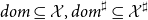
Solvers are meant to provide solutions to systems of equations over some complete lattice. Assume that
 $\mathcal{X}$
is a (not necessarily finite) set of unknowns and
$\mathcal{X}$
is a (not necessarily finite) set of unknowns and
 $\mathbb{D}$
a complete lattice. Then, a system of equations
$\mathbb{D}$
a complete lattice. Then, a system of equations
 $\mathbb{E}$
(with unknowns from
$\mathbb{E}$
(with unknowns from
 $\mathcal{X}$
and values in
$\mathcal{X}$
and values in
 $\mathbb{D}$
) assigns a right-hand side
$\mathbb{D}$
) assigns a right-hand side
 $F_x$
to each unknown
$F_x$
to each unknown
 $x\in\mathcal{X}$
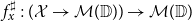
. Since we not only interested in the values assigned to unknowns but also in the dependencies between these, we assume that each right-hand side
$x\in\mathcal{X}$
. Since we not only interested in the values assigned to unknowns but also in the dependencies between these, we assume that each right-hand side
 $F_x$
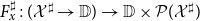
is a function of type
$F_x$
is a function of type
 $(\mathcal{X} \to \mathbb{D}) \to \mathbb{D} \times \mathcal{P} (\mathcal{X})$
.
$(\mathcal{X} \to \mathbb{D}) \to \mathbb{D} \times \mathcal{P} (\mathcal{X})$
.
-
The first component of the result of
 $F_x$
is the value for x;
$F_x$
is the value for x; -
The second component is a set of unknowns which is sufficient to determine the value.

More formally, we assume for the second component of
 $F_x$
that for every assignment
$F_x$
that for every assignment
 $\sigma:\mathcal{X}\to\mathbb{D}$
,
$\sigma:\mathcal{X}\to\mathbb{D}$
,
 $F_x\,\sigma = (d,X)$
implies that for any other assignment
$F_x\,\sigma = (d,X)$
implies that for any other assignment
 $\sigma':\mathcal{X}\to\mathbb{D}$
with
$\sigma':\mathcal{X}\to\mathbb{D}$
with
 $\sigma|_X = \sigma'|_X$
, that is, which agrees with
$\sigma|_X = \sigma'|_X$
, that is, which agrees with
 $\sigma$
on all unknowns from
$\sigma$
on all unknowns from
 $\mathcal{X}$
,
$\mathcal{X}$
,
 $F_x\,\sigma = F_x\,\sigma'$
holds as well.
$F_x\,\sigma = F_x\,\sigma'$
holds as well.
The set X thus can be considered as a superset of all unknowns onto which the unknown x depends – w.r.t. the assignment
 $\sigma$
. We remark this set very well may be different for different assignments. For convenience, we denote these two components of the result
$\sigma$
. We remark this set very well may be different for different assignments. For convenience, we denote these two components of the result
 $F_x\,\sigma$
as
$F_x\,\sigma$
as
 $(F_x\,\sigma)_1$
and
$(F_x\,\sigma)_1$
and
 $(F_x\,\sigma)_2$
, respectively.
$(F_x\,\sigma)_2$
, respectively.
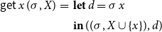
Systems of equations can be used to formulate the concrete (accumulating) semantics of a program. In this case, the complete lattice
 $\mathbb{D}$
is of the form
$\mathbb{D}$
is of the form
 $\mathcal{P} (\mathcal{Q})$
where
$\mathcal{P} (\mathcal{Q})$
where
 $\mathcal{Q}$
is the set of states possibly attained during program execution. Furthermore, all right-hand sides of the concrete semantics should be monotonic w.r.t. the natural ordering on pairs. This means that on larger assignments, the sets of states for x as well as the set of contributing unknowns may only increase.
$\mathcal{Q}$
is the set of states possibly attained during program execution. Furthermore, all right-hand sides of the concrete semantics should be monotonic w.r.t. the natural ordering on pairs. This means that on larger assignments, the sets of states for x as well as the set of contributing unknowns may only increase.
Example 1 For
 $\mathcal{X} = \mathcal{Q} = \mathbb{Z},$
a system of equations could have right-hand sides
$\mathcal{X} = \mathcal{Q} = \mathbb{Z},$
a system of equations could have right-hand sides
 $F_x:(\mathbb{Z} \to \mathcal{P} (\mathbb{Z})) \to (\mathcal{P} (\mathbb{Z}) \times \mathcal{P} (\mathbb{Z}))$
where, for example,
$F_x:(\mathbb{Z} \to \mathcal{P} (\mathbb{Z})) \to (\mathcal{P} (\mathbb{Z}) \times \mathcal{P} (\mathbb{Z}))$
where, for example,
 \begin{align*} F_1\,\sigma &= (\{0\}, \unicode{x00D8}) \\ F_2\,\sigma &= (\sigma\,1 \cup \sigma\,3, \{1,3\})\end{align*}
Thus,
 $F_1$
always returns the value
$F_1$
always returns the value
 $\{0\}$
and accordingly depends on no other unknown,
$\{0\}$
and accordingly depends on no other unknown,
 $F_2$
on the other hand returns the union of the values of unknowns 1 and 3. Therefore, it depends on both of them.
$F_2$
on the other hand returns the union of the values of unknowns 1 and 3. Therefore, it depends on both of them.
Example 2 As a running example, consider the program from Figure 1 which consists of the procedures main and p. Assume that these operate on a set
 $\mathcal{Q}$
of program states where the functions
$\mathcal{Q}$
of program states where the functions
 $h_1, h_2: \mathcal{Q} \to \mathcal{P} (\mathcal{Q})$
represent the semantics of basic computation steps. The collecting semantics for the program provides subsets of states for each program point
$h_1, h_2: \mathcal{Q} \to \mathcal{P} (\mathcal{Q})$
represent the semantics of basic computation steps. The collecting semantics for the program provides subsets of states for each program point
 $u \in {0, \ldots, 7}$
and each possible calling context
$u \in {0, \ldots, 7}$
and each possible calling context
 $q \in \mathcal{Q}$
. The right-hand side function
$q \in \mathcal{Q}$
. The right-hand side function
 $F_{{\langle{u,q}\rangle}}$
for each such pair
$F_{{\langle{u,q}\rangle}}$
for each such pair
 ${\langle{u,q}\rangle}$
is given by:
${\langle{u,q}\rangle}$
is given by:
 \begin{equation*}\begin{array}{lll}F_{{\langle{0,q}\rangle}}\,\sigma &=& (\{q\},\unicode{x00D8}) \\[0.5ex]F_{{\langle{1,q}\rangle}}\,\sigma &=& (\cup{h_1(q')\mid q'\in\sigma\,{\langle{0,q}\rangle}},\;{{\langle{0,q}\rangle}}) \\[0.5ex]F_{{\langle{2,q}\rangle}}\,\sigma &=& ({\textsf{combine}\,q_1\,q_2\mid q_1\in\sigma\,{\langle{1,q}\rangle}, q_2\in\sigma\,{\langle{7,q_1}\rangle}}, \\ & &\phantom{(}{{\langle{1,q}\rangle}}\cup{{\langle{7,q_1}\rangle}\mid q_1\in\sigma\,{\langle{1,q}\rangle}}) \\[0.5ex] F_{{\langle{3,q}\rangle}}\,\sigma &=& ({q},\unicode{x00D8}) \\[0.5ex]F_{{\langle{4,q}\rangle}}\,\sigma &=& (\sigma\,{\langle{3,q}\rangle},\;{{\langle{3,q}\rangle}}) \\[0.5ex]\end{array}\end{equation*}
 \begin{equation*}\begin{array}{lll}F_{{\langle{5,q}\rangle}}\,\sigma &=& (\cup{h_1(q_1)\mid q_1\in\sigma\,{\langle{4,q}\rangle}},{{\langle{4,q}\rangle}}) \\[0.5ex]F_{{\langle{6,q}\rangle}}\,\sigma &=& (\sigma\,{\langle{3,q}\rangle},\;{{\langle{3,q}\rangle}}) \\[0.5ex]F_{{\langle{7,q}\rangle}}\,\sigma &=& ({\textsf{combine}\,q_1\,q_2\mid q_1\in\sigma\,{\langle{5,q}\rangle}, q_2\in\sigma\,{\langle{7,q_1}\rangle}} \\ & &\phantom{(} \cup\,{h_2(q_1)\mid q_1\in\sigma\,{\langle{6,q}\rangle}}, \\ & &\phantom{(} {{\langle{5,q}\rangle}}\cup{{\langle{7,q_1}\rangle}\mid q_1\in\sigma\,{\langle{5,q}\rangle}}\cup {{\langle{6,q}\rangle}}) \end{array}\end{equation*}
Recall that in presence of local scopes of program variables, the state after a call may also depend on the state before the call. Accordingly, we use an auxiliary function
 $\textsf{combine}:\mathcal{Q}\to \mathcal{Q}\to \mathcal{Q}$
which determines the program state after a call from the state before the call and the state attained at the end of the procedure body. For simplicity, we have abandoned an extra function enter for modeling passing of parameters as considered, e.g., in Apinis et al. (Reference Apinis, Seidl, Vojdani and Igarashi2012) and thus assume that the full program state of the caller before the call is passed to the callee. If the set
$\textsf{combine}:\mathcal{Q}\to \mathcal{Q}\to \mathcal{Q}$
which determines the program state after a call from the state before the call and the state attained at the end of the procedure body. For simplicity, we have abandoned an extra function enter for modeling passing of parameters as considered, e.g., in Apinis et al. (Reference Apinis, Seidl, Vojdani and Igarashi2012) and thus assume that the full program state of the caller before the call is passed to the callee. If the set
 $\mathcal{Q}$
is of the form
$\mathcal{Q}$
is of the form
 $\mathcal{Q} = \mathcal{A}\times\mathcal{B}$
where
$\mathcal{Q} = \mathcal{A}\times\mathcal{B}$
where
 $\mathcal{A},\mathcal{B}$
are the sets of local and global states, respectively, the function
$\mathcal{A},\mathcal{B}$
are the sets of local and global states, respectively, the function
 $\textsf{combine}$
could, for example, be defined as
$\textsf{combine}$
could, for example, be defined as
 \begin{equation*}\textsf{combine}\,(a_1,b_1)\,(a_2,b_2) = (a_1,b_2)\end{equation*}
We remark that the sets of unknowns onto which the right-hand sides for
 ${\langle{2,q}\rangle}$
as well as
${\langle{2,q}\rangle}$
as well as
 ${\langle{7,q}\rangle}$
depend themselves depend on the assignment
${\langle{7,q}\rangle}$
depend themselves depend on the assignment
 $\sigma$
.
$\sigma$
.
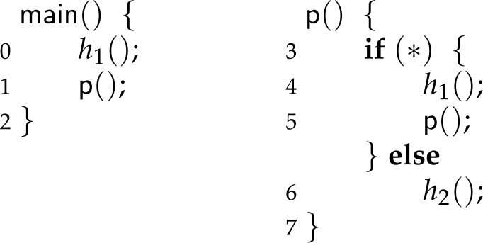
Figure 1. An example program with procedures.
Besides the concrete values provided for the unknowns, we also would like to determine the subset of unknowns which contribute to a particular subset of unknowns of interest. Restricting to this subset has the practical advantage that calculation may be restricted to a perhaps quite small number of unknowns only. Also, that subset in itself contains some form of reachability information. For interprocedural analysis, for example, of the program in Example 2, we are interested in all pairs
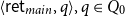 ${\langle\textsf{ret}_{\textit{main}},q\rangle},q\in Q_0$
, that is, the endpoint of the initially called procedure main for every initial calling context
${\langle\textsf{ret}_{\textit{main}},q\rangle},q\in Q_0$
, that is, the endpoint of the initially called procedure main for every initial calling context
 $q\in Q_0$
. In the Example 2, these would be of the form
$q\in Q_0$
. In the Example 2, these would be of the form
 ${\langle{2,q}\rangle}, q\in Q_0$
. In order to determine the sets of program states for the unknowns of interest, it suffices to consider only those calling contexts for each procedure p (and thus each program point within p) in which p is possibly called. The set of all such pairs is given as the least subset of unknowns which (directly or indirectly) influences any of the unknowns of interest.
${\langle{2,q}\rangle}, q\in Q_0$
. In order to determine the sets of program states for the unknowns of interest, it suffices to consider only those calling contexts for each procedure p (and thus each program point within p) in which p is possibly called. The set of all such pairs is given as the least subset of unknowns which (directly or indirectly) influences any of the unknowns of interest.
More technically for a system
 $\mathbb{E}$
of equations, consider an assignment
$\mathbb{E}$
of equations, consider an assignment
 $\sigma : \mathcal{X}\to \mathbb{D}$
and a subset
$\sigma : \mathcal{X}\to \mathbb{D}$
and a subset
 $\textit{dom}\subseteq\mathcal{X}$
of unknowns. Then,
$\textit{dom}\subseteq\mathcal{X}$
of unknowns. Then,
 $\textit{dom}$
is called
$\textit{dom}$
is called
 $(\sigma,\mathbb{E})$
-closed if
$(\sigma,\mathbb{E})$
-closed if
 $(F_x\,\sigma)_2\subseteq\textit{dom}$
is satisfied for all
$(F_x\,\sigma)_2\subseteq\textit{dom}$
is satisfied for all
 $x\in\textit{dom}$
. The pair
$x\in\textit{dom}$
. The pair
 $(\sigma,\textit{dom})$
is called a partial post-solution of
$(\sigma,\textit{dom})$
is called a partial post-solution of
 $\mathbb{E}$
, if
$\mathbb{E}$
, if
 $\textit{dom}$
is
$\textit{dom}$
is
 $(\sigma,\mathbb{E})$
-closed, and for each
$(\sigma,\mathbb{E})$
-closed, and for each
 $x\in\textit{dom}$
,
$x\in\textit{dom}$
,
 $\sigma\,x\sqsupseteq(F_x\,\sigma)_1$
holds.
$\sigma\,x\sqsupseteq(F_x\,\sigma)_1$
holds.
The partial post-solution
 $(\sigma,\textit{dom})$
of
$(\sigma,\textit{dom})$
of
 $\mathbb{E}$
is total (or just a post-solution of
$\mathbb{E}$
is total (or just a post-solution of
 $\mathbb{E}$
) if
$\mathbb{E}$
) if
 $\textit{dom}=\mathcal{X}$
. In this case, we also skip the second component in this pair.
$\textit{dom}=\mathcal{X}$
. In this case, we also skip the second component in this pair.
Example 3 Consider the following system of equations with
 $\mathcal{X} = \mathcal{Q} = \mathbb{Z}$
where
$\mathcal{X} = \mathcal{Q} = \mathbb{Z}$
where
 \begin{align*} F_1\,\sigma &= (\sigma\,2, \{2\}) \\ F_2\,\sigma &= (\{2\}, \unicode{x00D8}) \\ F_3\,\sigma &= (\{3\}, \unicode{x00D8}) \\ F_x\,\sigma &= (\unicode{x00D8},\unicode{x00D8})\qquad\text{otherwise}\end{align*}
Assume we are given the set of unknowns of interest
 $X = \{1\}$
. Then,
$X = \{1\}$
. Then,
 $(\sigma,\textit{dom})$
with
$(\sigma,\textit{dom})$
with
 $\textit{dom}=\{1,2\}$
,
$\textit{dom}=\{1,2\}$
,
 $\sigma\,1 = \{2\}$
and
$\sigma\,1 = \{2\}$
and
 $\sigma\,2= \{2\}$
is the least partial post-solution with
$\sigma\,2= \{2\}$
is the least partial post-solution with
 $X\subseteq\textit{dom}$
. For
$X\subseteq\textit{dom}$
. For
 $X' = \{1,3\}$
on the other hand, the least partial solution
$X' = \{1,3\}$
on the other hand, the least partial solution
 $(\sigma',\textit{dom}')$
with
$(\sigma',\textit{dom}')$
with
 $X'\subseteq\textit{dom}'$
is given by
$X'\subseteq\textit{dom}'$
is given by
 $\textit{dom}'=\{1,2,3\}$
and
$\textit{dom}'=\{1,2,3\}$
and
 $\sigma'\,1 = \{2\}, \sigma'\,2 = \{2\}$
and
$\sigma'\,1 = \{2\}, \sigma'\,2 = \{2\}$
and
 $\sigma'\,3 = \{3\}$
. For monotonic systems such as those used for representing the collecting semantics, and any set
$\sigma'\,3 = \{3\}$
. For monotonic systems such as those used for representing the collecting semantics, and any set
 $X\subseteq\mathcal{X}$
of unknowns of interest, there always exists a least partial solution comprising X.
$X\subseteq\mathcal{X}$
of unknowns of interest, there always exists a least partial solution comprising X.
Proposition 1 Assume that the system
 $\mathbb{E}$
of equations is monotonic. Then for each subset
$\mathbb{E}$
of equations is monotonic. Then for each subset
 $X\subseteq{\mathcal{X}}$
of unknowns, consider the set P of all partial post-solutions
$X\subseteq{\mathcal{X}}$
of unknowns, consider the set P of all partial post-solutions
 $(\sigma',{\textit{dom}}')\in (({\mathcal{X}}\to \mathbb{D})\times \mathcal{P} (\mathcal{X}))$
so that
$(\sigma',{\textit{dom}}')\in (({\mathcal{X}}\to \mathbb{D})\times \mathcal{P} (\mathcal{X}))$
so that
 $X\subseteq{\textit{dom}}'$
. Then, P has a unique least element
$X\subseteq{\textit{dom}}'$
. Then, P has a unique least element
 $(\sigma{}_X,{\textit{dom}}_X)$
. In particular,
$(\sigma{}_X,{\textit{dom}}_X)$
. In particular,
 $\sigma{}_X\,x'=\bot$
for all
$\sigma{}_X\,x'=\bot$
for all
 $x'\not\in\textit{dom}{}_X$
.
$x'\not\in\textit{dom}{}_X$
.
Proof. Consider the complete lattice
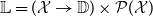 $\mathbb{L} = (\mathcal{X}\to\mathbb{D})\times \mathcal{P} (\mathcal{X})$
. The system
$\mathbb{L} = (\mathcal{X}\to\mathbb{D})\times \mathcal{P} (\mathcal{X})$
. The system
 $\mathbb{E}$
defines a function
$\mathbb{E}$
defines a function
 $F:\mathbb{L}\to\mathbb{L}$
by
$F:\mathbb{L}\to\mathbb{L}$
by
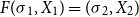 $F(\sigma{}_1,X_1) = (\sigma{}_2,X_2)$
where
$F(\sigma{}_1,X_1) = (\sigma{}_2,X_2)$
where
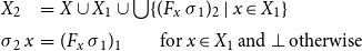 \begin{equation*}\begin{array}{lll}X_2 &=& X\cup X_1 \cup\bigcup\{ (F_x\,\sigma{}_1)_2 \mid x\in X_1\} \\\sigma{}_2\,x &=& (F_x\,\sigma{}_1)_1 \qquad\text{for}\;x\in X_1\;\text{and}\;\bot\;\text{otherwise}\end{array}\end{equation*}
Since each right-hand side
 $F_x$
in
$F_x$
in
 $\mathbb{E}$
is monotonic, so is the function F. Moreover,
$\mathbb{E}$
is monotonic, so is the function F. Moreover,
 $(\sigma,\textit{dom})$
is a post-fixpoint of F iff
$(\sigma,\textit{dom})$
is a post-fixpoint of F iff
 $(\sigma,\textit{dom})$
is a partial post-solution of
$(\sigma,\textit{dom})$
is a partial post-solution of
 $\mathbb{E}$
with
$\mathbb{E}$
with
 $X\subseteq\textit{dom}$
. By the fixpoint theorem of Knaster-Tarski, F has a unique least post-fixpoint – which happens to be also the least fixpoint of F.
$X\subseteq\textit{dom}$
. By the fixpoint theorem of Knaster-Tarski, F has a unique least post-fixpoint – which happens to be also the least fixpoint of F.
For a given set X, there thus is a least partial solution of
 $\mathbb{E}$
with a least domain
$\mathbb{E}$
with a least domain
 $\textit{dom}{}_X$
comprising X. Moreover for
$\textit{dom}{}_X$
comprising X. Moreover for
 $X\subseteq X'$
and least partial solutions
$X\subseteq X'$
and least partial solutions
 $(\sigma_X,\textit{dom}{}_X),(\sigma_{X'},\textit{dom}{}_{X'})$
comprising X and X’, respectively, we have
$(\sigma_X,\textit{dom}{}_X),(\sigma_{X'},\textit{dom}{}_{X'})$
comprising X and X’, respectively, we have
 $\textit{dom}{}_{X}\subseteq\textit{dom}{}_{X'}$
and
$\textit{dom}{}_{X}\subseteq\textit{dom}{}_{X'}$
and
 $\sigma_{X'}\,x = \sigma_X\,x$
for all
$\sigma_{X'}\,x = \sigma_X\,x$
for all
 $x\in\textit{dom}{}_X$
. In particular, this means for the least total solution
$x\in\textit{dom}{}_X$
. In particular, this means for the least total solution
 $\sigma$
that
$\sigma$
that
 $\sigma_X\,x = \sigma\,x$
whenever
$\sigma_X\,x = \sigma\,x$
whenever
 $x\in\textit{dom}{}_X$
.
$x\in\textit{dom}{}_X$
.
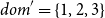
Example 4. Consider the program from Example 2. Assume that
 $\mathcal{Q}=\{q_0,q_1,q_2\}$
where the set of initial calling contexts is given by
$\mathcal{Q}=\{q_0,q_1,q_2\}$
where the set of initial calling contexts is given by
 $\{q_1\}$
. Accordingly, the set of unknowns of interest is given by
$\{q_1\}$
. Accordingly, the set of unknowns of interest is given by
 $X=\{{\langle2,q_1\rangle}\}$
(2 being the return point of main). Assume that the functions
$X=\{{\langle2,q_1\rangle}\}$
(2 being the return point of main). Assume that the functions
 $h_1,h_2$
are given by
$h_1,h_2$
are given by
 \begin{equation*}\begin{array}{lll}h_1 &=& \{ q_0\mapsto\unicode{x00D8}, q_1\mapsto\{q_2\}, q_2\mapsto\{q_0\}\} \\h_2 &=& \{ q_0\mapsto\{q_0\}, q_1\mapsto\unicode{x00D8}, q_2\mapsto\unicode{x00D8}\}\end{array}\end{equation*}
while the function combine always returns its second argument, that is,
 $\textsf{combine}\,q\,q' = q'$
.
$\textsf{combine}\,q\,q' = q'$
.
Let
 $\textit{dom}$
denote the set
$\textit{dom}$
denote the set
 \begin{equation*}\begin{array}{l}\{ {\langle0,q_1\rangle}, {\langle1,q_1\rangle}, {\langle2,q_1\rangle}, \\\;\;{\langle3,q_0\rangle}, {\langle4,q_0\rangle}, {\langle5,q_0\rangle}, {\langle6,q_0\rangle}, {\langle7,q_0\rangle}, \\\;\;{\langle3,q_2\rangle}, {\langle4,q_2\rangle}, {\langle5,q_2\rangle}, {\langle6,q_2\rangle}, {\langle7,q_2\rangle} \}. \\\end{array}\end{equation*}
Together with the assignment
 $\sigma : \textit{dom}\to \mathcal{P} (\mathcal{Q})\times \mathcal{P} (\mathcal{X})$
as shown in Figure 2, we obtain the least partial solution of the given system of equations which we refer to as the collecting semantics of the program. We remark that
$\sigma : \textit{dom}\to \mathcal{P} (\mathcal{Q})\times \mathcal{P} (\mathcal{X})$
as shown in Figure 2, we obtain the least partial solution of the given system of equations which we refer to as the collecting semantics of the program. We remark that
 $\textit{dom}$
only has calls of procedure p for the calling contexts
$\textit{dom}$
only has calls of procedure p for the calling contexts
 $q_0$
and
$q_0$
and
 $q_2$
.
$q_2$
.
Figure 2. The collecting semantics.
3. Abstract Systems of Equations
Systems of abstract equations are meant to provide sound information for concrete systems. In order to distinguish abstract systems from concrete ones, we usually use superscripts
 $\sharp$
at all corresponding entities. Abstract systems of equations differ from concrete ones in several aspects:
$\sharp$
at all corresponding entities. Abstract systems of equations differ from concrete ones in several aspects:
-
Right-hand side functions need no longer be monotonic.
-
Right-hand side functions should be effectively computable and thus may access the values only of finitely many other unknowns in the system (which need not be the case for concrete systems).
Example 5. Consider again the program from Figure 1 consisting of the procedures main and p. Assume that the abstract domain is given by some complete lattice
 $\mathbb{D}$
where the functions
$\mathbb{D}$
where the functions
 $h^\sharp_1 , h^\sharp_2 : \mathbb{D}\to\mathbb{D}$
represent the semantics of basic computation steps. The abstract semantics for the program provides an abstract state in
$h^\sharp_1 , h^\sharp_2 : \mathbb{D}\to\mathbb{D}$
represent the semantics of basic computation steps. The abstract semantics for the program provides an abstract state in
 $\mathbb{D}$
for each pair
$\mathbb{D}$
for each pair
 ${\langle u,a\rangle}$
(u program point from
${\langle u,a\rangle}$
(u program point from
 $\{ 0,\ldots,7\}$
, a possible abstract calling context from
$\{ 0,\ldots,7\}$
, a possible abstract calling context from
 $\mathbb{D}$
). The right-hand sides
$\mathbb{D}$
). The right-hand sides
 $F^\sharp{}_{{\langle u,a\rangle}}$
then are given by:
$F^\sharp{}_{{\langle u,a\rangle}}$
then are given by:
 \begin{equation*}\begin{array}{lll}F^\sharp{}_{{\langle0,a\rangle}}\,\sigma &=& (a,\unicode{x00D8}) \\[0.5ex]F^\sharp{}_{{\langle1,a\rangle}}\,\sigma &=& (h^\sharp{}_1\,(\sigma{\langle0,a\rangle}),\;{{\langle0,a\rangle}}) \\[0.5ex]F^\sharp{}_{{\langle2,a\rangle}}\,\sigma &=& (\textsf{combine}^\sharp\, (\sigma{\langle1,a\rangle})\, (\sigma{\langle7,\sigma{\langle1,a\rangle}\rangle}),\\[0.5ex] & & \quad{{\langle1,a\rangle},{\langle7,\sigma{\langle1,a\rangle}\rangle}}) \\[0.5ex]F^\sharp{}_{{\langle3,a\rangle}}\,\sigma &=& (a,\unicode{x00D8}) \\[0.5ex]F^\sharp{}_{{\langle4,a\rangle}}\,\sigma &=& (\sigma{\langle3,a\rangle},\;{{\langle3,a\rangle}}) \\[0.5ex]F^\sharp{}_{{\langle5,a\rangle}}\,\sigma &=& (h^\sharp{}_1\,(\sigma{\langle4,a\rangle}),{{\langle4,a\rangle}}) \\[0.5ex]F^\sharp{}_{{\langle6,a\rangle}}\,\sigma &=& (\sigma\,{\langle3,a\rangle},\,{{\langle3,a\rangle}}) \\[0.5ex]F^\sharp{}_{{\langle7,a\rangle}}\,\sigma &=& (\textsf{combine}^\sharp\,(\sigma{\langle5,a\rangle})\, (\sigma{\langle7, \sigma{\langle5,a\rangle}\rangle}) \sqcup\,h^\sharp{}_2\,(\sigma{\langle6,a\rangle}), \\ & &\phantom{(} {{\langle5,a\rangle}, {\langle7,\sigma{\langle5,a\rangle}\rangle}, {\langle6,a\rangle}}) \end{array}\end{equation*}
Corresponding to the function combine required by the collecting semantics, the auxiliary function
 $\textsf{combine}^\sharp:\mathbb{D}\to\mathbb{D}\to\mathbb{D}$
determines the abstract program state after a call from the abstract state before the call and the abstract state at the end of the procedure body.
$\textsf{combine}^\sharp:\mathbb{D}\to\mathbb{D}\to\mathbb{D}$
determines the abstract program state after a call from the abstract state before the call and the abstract state at the end of the procedure body.
Right-hand functions in practically given abstract systems of equations, however, usually do not explicitly provide a set of unknowns onto which the evaluation depends. Instead, the latter set is given implicitly via the implementation of the function computing the value for the left-hand side unknown. If necessary, this set must be determined by the solver, for example, as in case of TD, by keeping track of the unknowns accessed during the evaluation of the function.
Evaluation of the right-hand side function during solving may thus affect the internal state of the solver. Such operational behavior can conveniently be made explicit by means of state transformer monads. For a set S of (solver) states, the state transformer monad
 $\mathcal{M}_S(A)$
for values of type A consists of all functions
$\mathcal{M}_S(A)$
for values of type A consists of all functions
 $S\to S\times A$
. As a special case of a monad, the state transformer monad
$S\to S\times A$
. As a special case of a monad, the state transformer monad
 $\mathcal{M}_S(A)$
provides functions
$\mathcal{M}_S(A)$
provides functions
 $\textsf{return}: A \to \mathcal{M}_S(A)$
and
$\textsf{return}: A \to \mathcal{M}_S(A)$
and
 $\textsf{bind}: \mathcal{M}_S(A) \to (A\to\mathcal{M}_S(B)) \to \mathcal{M}_S(B)$
. These are defined by
$\textsf{bind}: \mathcal{M}_S(A) \to (A\to\mathcal{M}_S(B)) \to \mathcal{M}_S(B)$
. These are defined by
 \begin{equation*}\begin{array}{lll} \textsf{return}\,a &=& \textbf{fun}\,s\to (s,a) \\ \textsf{bind}\,m\,f &=& \textbf{fun}\,s\to \begin{array}[t]{l} \textbf{let}\,(s',a) = m\,s \\ \textbf{in}\, f\,a\,s' \end{array}\end{array}\end{equation*}
The solvers we consider only take actions when the current values of unknowns are accessed during the evaluation of right-hand sides. In the monadic formulation, the right-hand side functions
 $f^\sharp_x, x\in\mathcal{X}$
of the abstract system of equations
$f^\sharp_x, x\in\mathcal{X}$
of the abstract system of equations
 $\mathbb{E}^\sharp$
therefore are of type
$\mathbb{E}^\sharp$
therefore are of type
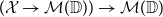 $(\mathcal{X}\to\mathcal{M}(\mathbb{D}))\to\mathcal{M}(\mathbb{D})$
for any monad
$(\mathcal{X}\to\mathcal{M}(\mathbb{D}))\to\mathcal{M}(\mathbb{D})$
for any monad
 $\mathcal{M}$
, that is, are parametric in
$\mathcal{M}$
, that is, are parametric in
 $\mathcal{M}$
(the system of equations should be ignorant of the internals of the solver!). Such functions
$\mathcal{M}$
(the system of equations should be ignorant of the internals of the solver!). Such functions
 $f^\sharp{}_x$
have been called pure in Karbyshev (Reference Karbyshev2013).
$f^\sharp{}_x$
have been called pure in Karbyshev (Reference Karbyshev2013).
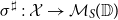
Example 6. For
 $\sigma^\sharp:\mathcal{X}\to\mathcal{M}_S(\mathbb{D})$
, the right-hand side functions in the monadic formulation of the abstract system of equations for the program from Figure 1 now are given by
$\sigma^\sharp:\mathcal{X}\to\mathcal{M}_S(\mathbb{D})$
, the right-hand side functions in the monadic formulation of the abstract system of equations for the program from Figure 1 now are given by
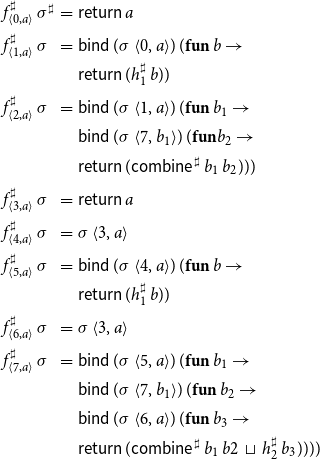 \begin{equation*}\begin{array}{lll}f^\sharp_{{\langle0,a\rangle}}\,\sigma^\sharp &=&\textsf{return}\,a \\[0.5ex]f^\sharp_{{\langle1,a\rangle}}\,\sigma &=& \textsf{bind}\,(\sigma\,{\langle0,a\rangle})\,(\textbf{fun}\,b\to \\ & & \textsf{return}\,(h^\sharp_1\,b)) \\[0.5ex]f^\sharp_{{\langle2,a\rangle}}\,\sigma &=& \textsf{bind}\,(\sigma\,{\langle1,a\rangle})\,(\textbf{fun}\,b_1\to\\ & & \textsf{bind}\,(\sigma\,{\langle7,b_1\rangle})\,(\textbf{fun} b_2 \to\\ & & \textsf{return}\,(\textsf{combine}^\sharp\,b_1\,b_2))) \\[0.5ex]f^\sharp_{{\langle3,a\rangle}}\,\sigma &=& \textsf{return}\,a \\[0.5ex]f^\sharp_{{\langle4,a\rangle}}\,\sigma &=& \sigma\,{\langle3,a\rangle} \\[0.5ex]f^\sharp_{{\langle5,a\rangle}}\,\sigma &=& \textsf{bind}\,(\sigma\,{\langle4,a\rangle})\,(\textbf{fun}\,b\to \\ & & \textsf{return}\,(h^\sharp_1\,b)) \\[0.5ex]f^\sharp_{{\langle6,a\rangle}}\,\sigma &=& \sigma\,{\langle3,a\rangle} \\[0.5ex]f^\sharp_{{\langle7,a\rangle}}\,\sigma &=& \textsf{bind}\,(\sigma\,{\langle5,a\rangle})\,(\textbf{fun}\,b_1\to \\ & & \textsf{bind}\,(\sigma\,{\langle7,b_1\rangle})\,(\textbf{fun}\,b_2\to \\ & & \textsf{bind}\,(\sigma\,{\langle6,a\rangle})\,(\textbf{fun}\,b_3\to \\ & & \textsf{return}\,(\textsf{combine}^\sharp\,b_1\,b2\;\sqcup\;h^\sharp_2\,b_3))))\end{array}\end{equation*}
According to the considerations in Karbyshev (Reference Karbyshev2013), each pure function f of type
 $(\mathcal{X}\to\mathcal{M}(\mathbb{D}))\to\mathcal{M}(\mathbb{D})$
equals the semantics
$(\mathcal{X}\to\mathcal{M}(\mathbb{D}))\to\mathcal{M}(\mathbb{D})$
equals the semantics
 ${t}$
of some computation tree t. Computation trees make explicit in which order the values of unknowns are queried when computing the result values of a function. The set of all computation trees (over the unknowns
${t}$
of some computation tree t. Computation trees make explicit in which order the values of unknowns are queried when computing the result values of a function. The set of all computation trees (over the unknowns
 $\mathcal{X}^\sharp$
and the set of values
$\mathcal{X}^\sharp$
and the set of values
 $\mathbb{D}$
) is the least set
$\mathbb{D}$
) is the least set
 $\mathcal{T}$
with
$\mathcal{T}$
with
 \begin{equation*}\mathcal{T}\quad{::=}\quad \textsf{A}\,\mathbb{D} \mid \textsf{Q}\,(\mathcal{X}^\sharp,\mathbb{D}\to\mathcal{T})\end{equation*}
The computation tree
 $\textsf{A}\,d$
immediately returns the answer d, while the computation tree
$\textsf{A}\,d$
immediately returns the answer d, while the computation tree
 $\textsf{Q}\,(x,f)$
queries the value of the unknown x in order to apply the continuation f to the obtained value.
$\textsf{Q}\,(x,f)$
queries the value of the unknown x in order to apply the continuation f to the obtained value.
Example 7 Consider again the program from Figure 1 consisting of the procedures main and p and the abstract system of equations as provided in Example 6. The computation trees
 $t_{{\langle u,a\rangle}}$
for the right-hand side functions
$t_{{\langle u,a\rangle}}$
for the right-hand side functions
 $f^\sharp_{{\langle u,a\rangle}}$
then are given by:
$f^\sharp_{{\langle u,a\rangle}}$
then are given by:
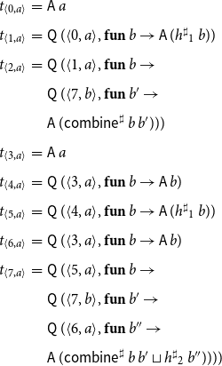 \begin{equation*}\begin{array}{lll}t_{{\langle0,a\rangle}} &=& \textsf{A}\,a \\[0.5ex]t_{{\langle1,a\rangle}} &=& \textsf{Q}\,({\langle0,a\rangle},\textbf{fun}\,b\to \textsf{A}\,(h^\sharp{}_1\,b)) \\[0.5ex]t_{{\langle2,a\rangle}} &=& \textsf{Q}\,({\langle1,a\rangle},\textbf{fun}\,b\to \\[0.5ex] & & \textsf{Q}\,({\langle7,b\rangle},\textbf{fun}\,b'\to \\[0.5ex] & & \textsf{A}\,(\textsf{combine}^\sharp\,b\,b'))) \\[0.5ex]t_{{\langle3,a\rangle}} &=& \textsf{A}\,a \\[0.5ex]t_{{\langle4,a\rangle}} &=& \textsf{Q}\,({\langle3,a\rangle},\textbf{fun}\,b\to \textsf{A}\,b) \\[0.5ex]t_{{\langle5,a\rangle}} &=& \textsf{Q}\,({\langle4,a\rangle},\textbf{fun}\,b\to \textsf{A}\,(h^\sharp{}_1\,b)) \\[0.5ex]t_{{\langle6,a\rangle}} &=& \textsf{Q}\,({\langle3,a\rangle},\textbf{fun}\,b\to \textsf{A}\,b) \\[0.5ex]t_{{\langle7,a\rangle}} &=& \textsf{Q}\,({\langle5,a\rangle},\textbf{fun}\,b\to \\[0.5ex] & & \textsf{Q}\,({\langle7,b\rangle},\textbf{fun}\,b'\to \\[0.5ex] & & \textsf{Q}\,({\langle6,a\rangle},\textbf{fun}\,b''\to\\[0.5ex] & & \textsf{A}\,(\textsf{combine}^\sharp\,b\,b'\sqcup h^\sharp{}_2\,b''))))\end{array}\end{equation*}
The semantics of a computation tree t is a function
 ${t}:(\mathcal{X}^\sharp\to\mathcal{M}(\mathbb{D}))\to \mathcal{M}(\mathbb{D})$
where for
${t}:(\mathcal{X}^\sharp\to\mathcal{M}(\mathbb{D}))\to \mathcal{M}(\mathbb{D})$
where for
 $\textsf{get}:\mathcal{X}\to\mathcal{M}(\mathbb{D})$
,
$\textsf{get}:\mathcal{X}\to\mathcal{M}(\mathbb{D})$
,
 \begin{equation*}\begin{array}{lll} {\textsf{A}\,d}\,\textsf{get} &=& \textsf{return}\,d \\ {\textsf{Q}\,(x,f)}\,\textsf{get} &=& \textsf{bind}\,(\textsf{get}\,x)\,(\textsf{fun}\,d\to{f\,d}\,\textsf{get}) \\ \end{array}\end{equation*}
In the particular case that
 $\mathcal{M}$
is the state transformer monad for a set of states S, we have:
$\mathcal{M}$
is the state transformer monad for a set of states S, we have:
 \begin{equation*}\begin{array}{lll} {\textsf{A}\,d}\,\textsf{get}\,s &=& (s,d) \\ {\textsf{Q}\,(x,f)}\,\textsf{get}\,s &=& \textbf{let}\;(s',d) = \textsf{get}\,x\,s \\ & & \textbf{in}\;{f\,d}\,\textsf{get}\,s' \\\end{array}\end{equation*}
When reasoning about (partial post-)solutions of abstract systems of equations, we prefer to have right-hand side functions where (a superset of) the set of accessed unknowns is explicit, as we used for concrete systems of equations. These functions, however, can be recovered from right-hand side functions in monadic form, as we indicate now.
One instance of state transformer monads is a monad which tracks the variables accessed during the evaluation. Consider the set of states
 $S = (\mathcal{X}^\sharp\to\mathbb{D})\times \mathcal{P} ({\mathcal{X}^\sharp})$
together with the function
$S = (\mathcal{X}^\sharp\to\mathbb{D})\times \mathcal{P} ({\mathcal{X}^\sharp})$
together with the function
 \begin{equation*}\begin{array}{lll} \textsf{get}\,x\,(\sigma,X) &=& \textbf{let}\;d = \sigma\,x \\ & & \textbf{in}\;((\sigma,X\cup\{x\}),d) \\\end{array}\end{equation*}
Proposition 2. For a mapping
 $\sigma : \mathcal{X}^\sharp\to\mathbb{D}$
and
$\sigma : \mathcal{X}^\sharp\to\mathbb{D}$
and
 $s=(\sigma,\unicode{x00D8})$
, assume that
$s=(\sigma,\unicode{x00D8})$
, assume that
 ${t}\;\textsf{get}\;s = (s_1,d)$
. Then for
${t}\;\textsf{get}\;s = (s_1,d)$
. Then for
 $s_1=(\sigma{}_1,X)$
the following holds:
$s_1=(\sigma{}_1,X)$
the following holds:
-
1.
$\sigma=\sigma{}_1$
; -
2. Assume that
$\sigma':\mathcal{X}^\sharp\to\mathbb{D}$
is another mapping and
$s'=(\sigma',\unicode{x00D8})$
. Let
${t}\;\textsf{get}\;s' = ((\sigma',X'),d')$
. If
$\sigma'$
agrees with
$\sigma$
on X, that is,
$\sigma|_X = \sigma'|_X$
, then
$X'=X$
and
$d'=d$
holds.


We strengthen the statement by claiming that the conclusions also hold when s and s’ are given by
 $(\sigma,X_0)$
and
$(\sigma,X_0)$
and
 $(\sigma',X_0)$
, respectively, for the same set
$(\sigma',X_0)$
, respectively, for the same set
 $X_0$
. Then, the proof is by induction on the structure of t.
$X_0$
. Then, the proof is by induction on the structure of t.
Now assume that for each abstract unknown
 $x\in\mathcal{X}^\sharp$
, the system
$x\in\mathcal{X}^\sharp$
, the system
 $\mathbb{E}^\sharp$
provides us with a right-hand side function
$\mathbb{E}^\sharp$
provides us with a right-hand side function
 $f^\sharp_x:(\mathcal{X}\to\mathcal{M}(\mathbb{D}))\to\mathcal{M}(\mathbb{D})$
. Then, the elaborated abstract right-hand side function
$f^\sharp_x:(\mathcal{X}\to\mathcal{M}(\mathbb{D}))\to\mathcal{M}(\mathbb{D})$
. Then, the elaborated abstract right-hand side function
 $F_x^\sharp : (\mathcal{X}^\sharp \to \mathbb{D}) \to \mathbb{D} \times \mathcal{P} ({\mathcal{X}^\sharp})$
of x is given by:
$F_x^\sharp : (\mathcal{X}^\sharp \to \mathbb{D}) \to \mathbb{D} \times \mathcal{P} ({\mathcal{X}^\sharp})$
of x is given by:
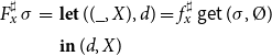 \begin{equation*}\begin{array}{lll}F_x^\sharp\,\sigma &=& \textbf{let}\;((\_,X),d) = f^\sharp_x\,\textsf{get}\,(\sigma,\unicode{x00D8}) \\& & \textbf{in}\; (d,X)\end{array}\end{equation*}
In fact, the explicit right-hand side functions
 $F^\sharp_{{\langle u,a\rangle}}$
of Example 5 are obtained in this way from the functions
$F^\sharp_{{\langle u,a\rangle}}$
of Example 5 are obtained in this way from the functions
 $f^\sharp_{{\langle u,a\rangle}}$
of Example 6.
$f^\sharp_{{\langle u,a\rangle}}$
of Example 6.
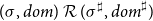
In order to relate the abstract with a corresponding concrete system of equations, we assume that there is a Galois connection (Cousot and Cousot Reference Cousot, Cousot, Graham, Harrison and Sethi1977) between the complete lattices
 $\mathcal{P} (\mathcal{Q})$
and
$\mathcal{P} (\mathcal{Q})$
and
 $\mathbb{D}$
, that is, monotonic mappings
$\mathbb{D}$
, that is, monotonic mappings
 $\alpha : \mathcal{P} (\mathcal{Q})\to\mathbb{D}$
(the abstraction) and
$\alpha : \mathcal{P} (\mathcal{Q})\to\mathbb{D}$
(the abstraction) and
 $\gamma : \mathbb{D}\to \mathcal{P} (\mathcal{Q})$
(the concretization) so that
$\gamma : \mathbb{D}\to \mathcal{P} (\mathcal{Q})$
(the concretization) so that
 \begin{equation*}\alpha\,Q\sqsubseteq a\qquad\text{iff}\qquad Q\subseteq\gamma\,a\end{equation*}
holds for all
 $Q\in\mathcal{P} (\mathcal{Q})$
and
$Q\in\mathcal{P} (\mathcal{Q})$
and
 $a\in\mathbb{D}$
.
$a\in\mathbb{D}$
.
In general, the sets of unknowns of the concrete system to be analyzed and the corresponding abstract system need not coincide. For interprocedural context-sensitive analysis, for example, the set of concrete unknowns is given by the set of all pairs
 ${\langle{u,q}\rangle}$
where u is a program point and
${\langle{u,q}\rangle}$
where u is a program point and
 $q\in\mathcal{Q}$
is a program state. The set of abstract unknowns are of the same form. The second components of pairs, however, now represent abstract calling contexts. Therefore, we assume that we are given a description relation
$q\in\mathcal{Q}$
is a program state. The set of abstract unknowns are of the same form. The second components of pairs, however, now represent abstract calling contexts. Therefore, we assume that we are given a description relation
 $\mathrel{\mathcal{R}} \subseteq \mathcal{X} \times \mathcal{X}^\sharp$
between the concrete and abstract unknowns. In case of interprocedural analysis, for example, we define
$\mathrel{\mathcal{R}} \subseteq \mathcal{X} \times \mathcal{X}^\sharp$
between the concrete and abstract unknowns. In case of interprocedural analysis, for example, we define
 $\mathrel{\mathcal{R}}$
by
$\mathrel{\mathcal{R}}$
by
 \begin{equation*}{\langle{u,q}\rangle} \mathrel{\mathcal{R}} {\langle u,a\rangle}\quad\text{iff}\quad q\in\gamma(a)\end{equation*}
Using the concretization
 $\gamma$
, the description relation
$\gamma$
, the description relation
 $\mathrel{\mathcal{R}}$
on unknowns is extended as follows.
$\mathrel{\mathcal{R}}$
on unknowns is extended as follows.
-
For sets of unknowns
$Y\subseteq\mathcal{X}$
and
$Y^\sharp\subseteq\mathcal{X}^\sharp$
,
$Y\mathrel{\mathcal{R}} Y^\sharp$
iff for each
$y\in Y$
,
$y\mathrel{\mathcal{R}} y^\sharp$
for some
$y^\sharp\in Y^\sharp$
. -
For sets of states
$Q\in\mathcal{P} (\mathcal{Q})$
and
$d\in\mathbb{D}$
,
$Q\mathrel{\mathcal{R}} d$
iff
$Q\subseteq\gamma\,d$
; -
For partial assignments
$(\sigma,\textit{dom})$
and
$(\sigma^\sharp,\textit{dom}^\sharp)$
with
$\sigma : \mathcal{X}\to\mathbb{D},\sigma^\sharp : \mathcal{X}^\sharp\to\mathbb{D}^\sharp$
and
$\textit{dom}\subseteq\mathcal{X},\textit{dom}^\sharp\subseteq\mathcal{X}^\sharp$
,
$(\sigma,\textit{dom})\mathrel{\mathcal{R}}(\sigma^\sharp,\textit{dom}^\sharp)$
holds if
$\textit{dom}\mathrel{\mathcal{R}}\textit{dom}^\sharp$
, and for all
$y\in\textit{dom}$
,
$y\in\textit{dom}^\sharp$
with
$y\mathrel{\mathcal{R}} y^\sharp$
,
$\sigma\,y\subseteq\gamma(\sigma^\sharp\,y^\sharp)$
. -
For (elaborated) right-hand sides
$F : (\mathcal{X}\to \mathcal{P} ({\mathcal{Q}}))\to(\mathcal{P} (\mathcal{Q})\times \mathcal{P} (\mathcal{X}))$
and
$F^\sharp : (\mathcal{X}^\sharp\to \mathbb{D})\to(\mathbb{D}\times \mathcal{P} ({\mathcal{X}^\sharp}))$
,
$F\mathrel{\mathcal{R}} F^\sharp$
iff
$(F\,\sigma)_1\subseteq\gamma\,(F^\sharp\,\sigma^\sharp)_1$
, and
$(F\,\sigma)_2\mathrel{\mathcal{R}}(F^\sharp\,\sigma^\sharp)_2$
whenever
$(\sigma,\textit{dom})\mathrel{\mathcal{R}}(\sigma^\sharp,\textit{dom}^\sharp)$
holds for domains
$\textit{dom},\textit{dom}^\sharp$
which are
$(\sigma,\mathbb{E})$
-closed and
$(\sigma^\sharp,\mathbb{E}^\sharp)$
-closed, respectively. -
For equation systems
$\mathbb{E} : \mathcal{X} \to ((\mathcal{X}\to \mathcal{P} ({\mathcal{Q}}))\to(\mathcal{P} (\mathcal{Q})\times \mathcal{P} (\mathcal{X})))$
and
$\mathbb{E}^\sharp : \mathcal{X}^\sharp \to ((\mathcal{X}^\sharp\to \mathcal{M}_S(\mathbb{D}))\to\mathcal{M}_S(\mathbb{D}))$
,
$\mathbb{E} \mathrel{\mathcal{R}} \mathbb{E}^\sharp$
iff
$(\mathbb{E}\,x) \mathrel{\mathcal{R}} F^\sharp{}_{x^\sharp}$
for each
$x \in \mathcal{X}$
,
$x^\sharp \in \mathcal{X}^\sharp$
, where
$F^\sharp{}_{x^\sharp}$
is the elaboration of
$\mathbb{E}^\sharp\,x^\sharp$
.


Let
 $(\sigma,\textit{dom})$
be the least solution of the concrete system
$(\sigma,\textit{dom})$
be the least solution of the concrete system
 $\mathbb{E}$
for some set X of interesting unknowns. Let
$\mathbb{E}$
for some set X of interesting unknowns. Let
 $\mathbb{E}^\sharp$
denote an abstract system corresponding to
$\mathbb{E}^\sharp$
denote an abstract system corresponding to
 $\mathbb{E}$
and
$\mathbb{E}$
and
 $X^\sharp$
a set of abstract unknowns and
$X^\sharp$
a set of abstract unknowns and
 $\mathrel{\mathcal{R}}$
a description relation between the unknowns of
$\mathrel{\mathcal{R}}$
a description relation between the unknowns of
 $\mathbb{E}$
and
$\mathbb{E}$
and
 $\mathbb{E}^\sharp$
such that
$\mathbb{E}^\sharp$
such that
 $\mathbb{E}\;\mathrel{\mathcal{R}}\;\mathbb{E}^\sharp$
and
$\mathbb{E}\;\mathrel{\mathcal{R}}\;\mathbb{E}^\sharp$
and
 $X\;\mathrel{\mathcal{R}}\;X^\sharp$
holds. A local solver then determines for
$X\;\mathrel{\mathcal{R}}\;X^\sharp$
holds. A local solver then determines for
 $\mathbb{E}^\sharp$
and
$\mathbb{E}^\sharp$
and
 $X^\sharp$
a pair
$X^\sharp$
a pair
 $(\sigma^\sharp,\textit{dom}^\sharp)$
so that
$(\sigma^\sharp,\textit{dom}^\sharp)$
so that
 $X\subseteq\textit{dom}^\sharp$
,
$X\subseteq\textit{dom}^\sharp$
,
 $\textit{dom}^\sharp$
is
$\textit{dom}^\sharp$
is
 $\sigma^\sharp$
-closed and
$\sigma^\sharp$
-closed and
 $(\sigma,\textit{dom})\;\mathrel{\mathcal{R}}\;(\sigma^\sharp,\textit{dom}^\sharp)$
holds, that is, the result produced by the solver is a sound description of the least partial solution of the concrete system.
$(\sigma,\textit{dom})\;\mathrel{\mathcal{R}}\;(\sigma^\sharp,\textit{dom}^\sharp)$
holds, that is, the result produced by the solver is a sound description of the least partial solution of the concrete system.
In absence of narrowing, the correctness of a solver can be proven intrinsically, that is, just by verifying that it terminates with a post-solution of the system of equations.
We first convince ourselves that the following holds:
Proposition 3. Assume that
 $\mathbb{E}\mathrel{\mathcal{R}}\mathbb{E}^\sharp$
holds and
$\mathbb{E}\mathrel{\mathcal{R}}\mathbb{E}^\sharp$
holds and
 $X\mathrel{\mathcal{R}} X^\sharp$
for subsets X and
$X\mathrel{\mathcal{R}} X^\sharp$
for subsets X and
 $X^\sharp$
concrete and abstract unknowns, respectively. Assume that
$X^\sharp$
concrete and abstract unknowns, respectively. Assume that
 $(\sigma,\textit{dom})$
is the least partial post-solution of
$(\sigma,\textit{dom})$
is the least partial post-solution of
 $\mathbb{E}$
with
$\mathbb{E}$
with
 $X\subseteq\textit{dom}$
, and
$X\subseteq\textit{dom}$
, and
 $(\sigma^\sharp,\textit{dom}^\sharp)$
some partial post-solution of
$(\sigma^\sharp,\textit{dom}^\sharp)$
some partial post-solution of
 $\mathbb{E}^\sharp$
with
$\mathbb{E}^\sharp$
with
 $X^\sharp\subseteq\textit{dom}^\sharp$
. Then
$X^\sharp\subseteq\textit{dom}^\sharp$
. Then
 $(\sigma,\textit{dom})\mathrel{\mathcal{R}}(\sigma^\sharp,\textit{dom}^\sharp)$
holds.
$(\sigma,\textit{dom})\mathrel{\mathcal{R}}(\sigma^\sharp,\textit{dom}^\sharp)$
holds.
Proposition 3 is a special case of Proposition 4 where additionally side effects and dynamic description relations are taken into account. Therefore, the proof of Proposition 3 is omitted. Proposition 3 can be used to prove soundness for local solver algorithms which perform accumulating fixpoint iteration and thus return partial post-solutions. These kinds of solvers require abstract domains where strictly ascending chains are always finite. This assumption, however, is no longer met for more complicated domains such as the interval domain (Cousot and Cousot Reference Cousot, Cousot, Graham, Harrison and Sethi1977) or octagons (Mine 2001). As already observed in Cousot and Cousot (Reference Cousot, Cousot, Graham, Harrison and Sethi1977), their applicability to these domains can still be extended by introducing widening operators. According to Cousot and Cousot (Reference Cousot and Cousot1992), Cousot (Reference Cousot, D’Souza, Lal and Larsen2015), a widening operator
 $\nabla$
is a mapping
$\nabla$
is a mapping
 $\nabla : \mathbb{D}\times\mathbb{D}\to\mathbb{D}$
with the following two properties:
$\nabla : \mathbb{D}\times\mathbb{D}\to\mathbb{D}$
with the following two properties:
-
(1).
$a\sqcup b\sqsubseteq a\nabla b$
for all
$a,b\in\mathbb{D}$
; -
(2). Every sequence
$a_0,a_1,\ldots $
defined by
$a_{i+1} = a_i\nabla b_i$
,
$i\geq 0$
for any
$b_i\in\mathbb{D}$
is ultimately stable.


Acceleration with widening then means that the occurrences of
 $\sqcup$
in the solver are replaced with
$\sqcup$
in the solver are replaced with
 $\nabla$
.
$\nabla$
.
Example 8. For intervals over
 $\mathbb{Z}{}_{-\infty}^{+\infty}$
we could use primitive widening:
$\mathbb{Z}{}_{-\infty}^{+\infty}$
we could use primitive widening:
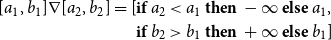 \begin{align*} [a_1, b_1] \nabla [a_2, b_2] = [&\textbf{if }a_2
< a_1 \textbf{ then } -\infty \textbf{ else } a_1, \\ &\textbf{if }b_2 > b_1 \textbf{ then } +\infty \textbf{ else } b_1]\end{align*}
\begin{align*} [a_1, b_1] \nabla [a_2, b_2] = [&\textbf{if }a_2
< a_1 \textbf{ then } -\infty \textbf{ else } a_1, \\ &\textbf{if }b_2 > b_1 \textbf{ then } +\infty \textbf{ else } b_1]\end{align*}
Alternatively, we could use threshold widening where several intermediate bounds are introduced that can be jumped to. Note that widening in general is not monotonic in the first argument:
 $[0,1] \sqsubseteq [0,2]$
but
$[0,1] \sqsubseteq [0,2]$
but
 $[0,1] \nabla [0,2] = [0, +\infty] \not\sqsubseteq [0,2] = [0,2] \nabla [0,2]$
. We remark that Cousot and Cousot (Reference Cousot and Cousot1992), Cousot (Reference Cousot, D’Souza, Lal and Larsen2015) provide a more general notion of widening which refers not to the ordering of
$[0,1] \nabla [0,2] = [0, +\infty] \not\sqsubseteq [0,2] = [0,2] \nabla [0,2]$
. We remark that Cousot and Cousot (Reference Cousot and Cousot1992), Cousot (Reference Cousot, D’Souza, Lal and Larsen2015) provide a more general notion of widening which refers not to the ordering of
 $\mathbb{D}$
but (via
$\mathbb{D}$
but (via
 $\gamma$
) to the ordering in the concrete lattice
$\gamma$
) to the ordering in the concrete lattice
 $\mathcal{P} (\mathcal{Q})$
alone. W.r.t. that definition,
$\mathcal{P} (\mathcal{Q})$
alone. W.r.t. that definition,
 $a\sqcup b$
is no longer necessarily less or equal
$a\sqcup b$
is no longer necessarily less or equal
 $a\nabla b$
. In many applications, however, accelerated loss of precision due to widening may result in unacceptable analysis results. Therefore, Cousot and Cousot (Reference Cousot, Cousot, Graham, Harrison and Sethi1977) proposed to complement a terminating widening iteration with a narrowing iteration which subsequently tries to recover some of the precision loss. Following Cousot and Cousot (Reference Cousot and Cousot1992), Cousot (Reference Cousot, D’Souza, Lal and Larsen2015), a narrowing operator
$a\nabla b$
. In many applications, however, accelerated loss of precision due to widening may result in unacceptable analysis results. Therefore, Cousot and Cousot (Reference Cousot, Cousot, Graham, Harrison and Sethi1977) proposed to complement a terminating widening iteration with a narrowing iteration which subsequently tries to recover some of the precision loss. Following Cousot and Cousot (Reference Cousot and Cousot1992), Cousot (Reference Cousot, D’Souza, Lal and Larsen2015), a narrowing operator
 $\Delta$
is a mapping
$\Delta$
is a mapping
 $\Delta : \mathbb{D}\times\mathbb{D}\to\mathbb{D}$
with the following two properties:
$\Delta : \mathbb{D}\times\mathbb{D}\to\mathbb{D}$
with the following two properties:
-
(1).
$a\sqcap b\sqsubseteq(a\Delta b)\sqsubseteq a$
for all
$a,b\in\mathbb{D}$
; -
(2). Every sequence
$a_0,a_1,\ldots $
defined by
$a_{i+1} = a_i\Delta b_i$
,
$i\geq 0$
for any
$b_i\in\mathbb{D}$
is ultimately stable.


Example 9. For intervals over
 $\mathbb{Z}{}_{-\infty}^{+\infty}$
we could use primitive narrowing:
$\mathbb{Z}{}_{-\infty}^{+\infty}$
we could use primitive narrowing:
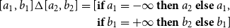 \begin{align*} [a_1, b_1] \Delta [a_2, b_2] = [&\textbf{if }a_1 = -\infty \textbf{ then } a_2 \textbf{ else } a_1, \\ &\textbf{if }b_1 = +\infty \textbf{ then } b_2 \textbf{ else } b_1]\end{align*}
which improves infinite bounds only. More sophisticated narrowing operators may allow a bounded number of improvements of finite bounds as well. Again we remark that, according to the more general definition in Cousot and Cousot (Reference Cousot and Cousot1992), Cousot (Reference Cousot, D’Souza, Lal and Larsen2015), the first property need not necessarily be satisfied. For monotonic systems of equations, the narrowing iteration when starting with a (partial) post-solution still will return a (partial) post-solution. The correctness of the solver started with an initial query
 $x^\sharp$
and returning a partial assignment
$x^\sharp$
and returning a partial assignment
 $\sigma^\sharp$
with domain
$\sigma^\sharp$
with domain
 $\textit{dom}^\sharp$
thus can readily be checked by verifying that
$\textit{dom}^\sharp$
thus can readily be checked by verifying that
-
1.
$x^\sharp\in\textit{dom}^\sharp$
; -
2.
$(F^\sharp{}_x\,\sigma^\sharp)_2\subseteq\textit{dom}^\sharp$
for all
$x\in\textit{dom}^\sharp$
, that is,
$\textit{dom}^\sharp$
is
$(\sigma^\sharp,\mathbb{E}^\sharp)$
-closed; and -
3.
$\sigma^\sharp\,x\sqsupseteq(F^\sharp{}_x\,\sigma^\sharp)_1$
for all
$x\in\textit{dom}^\sharp$
.


When the system of equations is non-monotonic, though, the computed assignment still is a sound description. It is, however, no longer guaranteed to be a post-solution of
 $\mathbb{E}^\sharp$
. In Section 6, we come back to this point.
$\mathbb{E}^\sharp$
. In Section 6, we come back to this point.
4. The Terminating Solver TDterm
In this section, we present our modification to the TD solver with widening and narrowing which improves on the variant in Apinis et al. (Reference Apinis, Seidl, Vojdani, Probst, Hankin and Hansen2016) in that termination guarantees can be proven even for non-monotonic abstract systems of equations. The vanilla TD solver from Muthukumar and Hermenegildo (Reference Muthukumar and Hermenegildo1990), Charlier and Van Hentenryck (Reference Charlier and Van Hentenryck1992) (see Appendix A for a pseudo code formulation of this solver along the lines presented in Fecht and Seidl Reference Fecht and Seidl1999) starts by querying the value of a given unknown. In order to answer the query, the solver evaluates the corresponding right-hand side. Whenever in the course of that evaluation, the value of another unknown is required, the best possible value for that unknown is computed first, before evaluation of the current right-hand side continues. Interestingly, the strategy employed by TD for choosing the next unknown to iterate upon, thereby resembles the iteration orders considered in Bourdoncle (Reference Bourdoncle, Bjørner, Broy and Pottosin1993) (see Fecht and Seidl Reference Fecht and Seidl1999 for a detailed comparison) for systems of equations derived from control-flow graphs of programs. The most remarkable difference, however, is that TD determines its order on-the-fly, while the ordering in Bourdoncle (Reference Bourdoncle, Bjørner, Broy and Pottosin1993) is determined via preprocessing.
In Apinis et al. (Reference Apinis, Seidl, Vojdani, Probst, Hankin and Hansen2016), the vanilla TD solver from Muthukumar and Hermenegildo (Reference Muthukumar and Hermenegildo1990), Charlier and Van Hentenryck (Reference Charlier and Van Hentenryck1992), Fecht and Seidl (Reference Fecht and Seidl1999) is enhanced with widening and narrowing. For that, the solver is equipped with a novel technique for identifying not only accesses to unknowns, but also widening and narrowing points on-the-fly. Moreover, that solver does not delegate the narrowing iteration to a separate second phase (as was done in the original papers on widening and narrowing Cousot and Cousot Reference Cousot and Cousot1992; Cousot Reference Cousot, D’Souza, Lal and Larsen2015), once a proceeding widening iteration has completed. Instead, widening and narrowing iterations may occur intertwined (Amato et al. Reference Amato, Scozzari, Seidl, Apinis and Vojdani2016). This is achieved by combining the widening operator
 $\nabla$
with the narrowing operator
$\nabla$
with the narrowing operator
 $\Delta$
into a single warrowing operator
$\Delta$
into a single warrowing operator
 $\unicode{x29C4}$
:
$\unicode{x29C4}$
:
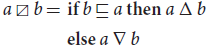 \begin{equation*}a\unicode{x29C4} b = \begin{array}[t]{l} \textbf{if}\; b\sqsubseteq a\;\textbf{then}\;a\Delta b\\ \textbf{else}\;a\nabla b \end{array}\end{equation*}
This operator applies
 $\Delta$
whenever values decrease and otherwise applies
$\Delta$
whenever values decrease and otherwise applies
 $\nabla$
.
$\nabla$
.
In Apinis et al. (Reference Apinis, Seidl, Vojdani, Probst, Hankin and Hansen2016), it is proven that solver TD (in the formulation of Fecht and Seidl Reference Fecht and Seidl1999) and equipped with warrowing at dynamically detected widening/narrowing points terminates for monotonic systems – whenever only finitely many unknowns are encountered. Example 10, though, shows a non-monotonic system for which this solver does not terminate – while the new solver
 $\mathbf{TD}_{\mathbf{term}}$
does.
$\mathbf{TD}_{\mathbf{term}}$
does.
Example 10. Consider the single equation:
 \begin{equation*}x = \textsf{if}\, x = 0 \,\textsf{then}\, 1 \,\textsf{else}\, 0\end{equation*}
over the lattice of naturals (with infinity) with
 $a \nabla b = \infty$
whenever
$a \nabla b = \infty$
whenever
 $a < b$
and
$a < b$
and
 $a \Delta b = b$
whenever
$a \Delta b = b$
whenever
 $a = \infty$
. The right-hand side of this equation is not monotonic. An iteration with warrowing leads to the sequence of values for x
$a = \infty$
. The right-hand side of this equation is not monotonic. An iteration with warrowing leads to the sequence of values for x
 \begin{equation*}0 \to \infty \to 0 \to \infty \to \ldots\end{equation*}
and thus will not terminate.
In order to deal with non-monotonic systems, we do no longer rely on warrowing. Instead, we equip the solver with extra logic to switch for each unknown from widening to narrowing (and never back). Our new solver is presented as OCaml pseudocode operating on abstract systems of equations. W.l.o.g., we also assume that solving starts with a single unknown of interest. In case that simultaneously values for unknowns from an arbitrary finite set X are of interest, we may introduce an artificial fresh unknown
 $x_0$
whose right-hand side successively queries the values of
$x_0$
whose right-hand side successively queries the values of
 $x\in X$
.
$x\in X$
.
For better readability, the solver state is not threaded through the evaluation of right-hand sides by means of a monad, but realized by mutable data structures:
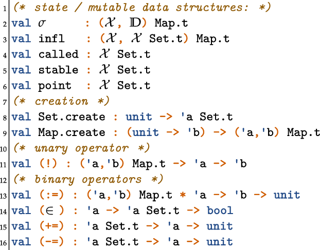
Here, the functional argument f to the function Map.create is meant to return an initial value
 $f\;()$
for a key which has not yet been assigned in the given map data structure.
$f\;()$
for a key which has not yet been assigned in the given map data structure.
Under that proviso, the OCaml type of a right-hand side function
 $f^\sharp_x$
thus is just
$f^\sharp_x$
thus is just
 $(\mathcal{X}\to\mathbb{D})\to\mathbb{D}$
. When reasoning about the values computed by right-hand sides as well as the sets of unknowns accessed during the evaluation, we will refer to the elaborated right-hand sides
$(\mathcal{X}\to\mathbb{D})\to\mathbb{D}$
. When reasoning about the values computed by right-hand sides as well as the sets of unknowns accessed during the evaluation, we will refer to the elaborated right-hand sides
 $F^\sharp_x$
corresponding to the
$F^\sharp_x$
corresponding to the
 $f^\sharp_x$
. The solver itself consists of three functions: the function solve which performs the iteration for a given unknown x; the function eval which wraps lookups of values of unknowns in the current state; and finally, the function destabilize which marks encountered unknowns possibly affected by a change to the value of some unknown, for re-evaluation.
$f^\sharp_x$
. The solver itself consists of three functions: the function solve which performs the iteration for a given unknown x; the function eval which wraps lookups of values of unknowns in the current state; and finally, the function destabilize which marks encountered unknowns possibly affected by a change to the value of some unknown, for re-evaluation.
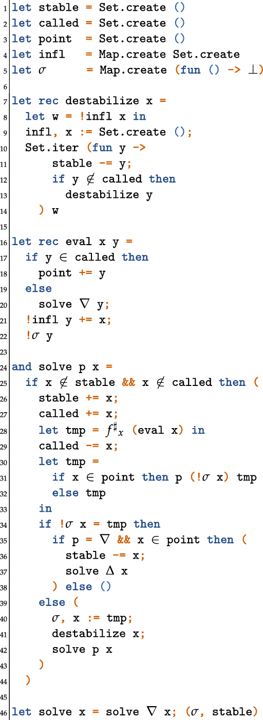
We briefly sketch the intuition behind this algorithm. The set
 $\textit{called}$
is the set of all unknowns where iteration currently is in progress, that is, which are contained in the call stack of the solver. The set
$\textit{called}$
is the set of all unknowns where iteration currently is in progress, that is, which are contained in the call stack of the solver. The set
 $\textit{stable}$
on the other hand consists of all unknowns where the iteration (relative to the current values of unknowns on the call stack) has terminated. For unknowns in any of these two sets, solving should immediately terminate.
$\textit{stable}$
on the other hand consists of all unknowns where the iteration (relative to the current values of unknowns on the call stack) has terminated. For unknowns in any of these two sets, solving should immediately terminate.
A key issue is to propagate the information that the value of some unknown y has changed, to all unknowns whose right-hand sides have been evaluated under wrong assumptions on y. A key ingredient both of the original TD solver and the variant in Apinis et al. (Reference Apinis, Seidl, Vojdani, Probst, Hankin and Hansen2016) is that dependences between unknowns are dynamically detected and recorded in the map
 $\textit{infl}:\mathcal{X}^\sharp\to \mathcal{P} ({\mathcal{X}^\sharp})$
. The set
$\textit{infl}:\mathcal{X}^\sharp\to \mathcal{P} ({\mathcal{X}^\sharp})$
. The set
 $\textit{infl}\,y$
is meant to record the set of unknowns x where the evaluation of
$\textit{infl}\,y$
is meant to record the set of unknowns x where the evaluation of
 $f^\sharp{}_x$
has accessed the current value of y, that is, where y influences x.
$f^\sharp{}_x$
has accessed the current value of y, that is, where y influences x.
As soon as the value of an unknown y is changed, therefore, the function
 $\textsf{destabilize}$
is called.
$\textsf{destabilize}$
is called.
 $\textsf{destabilize}\,y$
removes all unknowns directly or indirectly influenced by y from the set
$\textsf{destabilize}\,y$
removes all unknowns directly or indirectly influenced by y from the set
 $\textit{stable}$
. That recursive removal only stops at unknowns which are contained in the set
$\textit{stable}$
. That recursive removal only stops at unknowns which are contained in the set
 $\textit{called}$
. We remark that by the call
$\textit{called}$
. We remark that by the call
 $\textsf{destabilize}\,y$
, also the set
$\textsf{destabilize}\,y$
, also the set
 $\textit{infl}\,y$
is reset to
$\textit{infl}\,y$
is reset to
 $\unicode{x00D8}$
.
$\unicode{x00D8}$
.
The current values for unknowns are maintained in the map
 $\sigma$
. In order to track dependences between unknowns, we wrap the access to entries in
$\sigma$
. In order to track dependences between unknowns, we wrap the access to entries in
 $\sigma$
into the call
$\sigma$
into the call
 $\textsf{eval}\,x$
where x is the unknown in whose right-hand side the values in
$\textsf{eval}\,x$
where x is the unknown in whose right-hand side the values in
 $\sigma$
are queried. Thus, a call
$\sigma$
are queried. Thus, a call
 $\textsf{eval}\,x\,y$
ultimately returns the latest value in
$\textsf{eval}\,x\,y$
ultimately returns the latest value in
 $\sigma$
for y. Before that, however, it checks whether
$\sigma$
for y. Before that, however, it checks whether
 $y\in\textit{called}$
holds. If this is the case, y is turned into an unknown where widening and narrowing is applied. All these unknowns are collected into the set
$y\in\textit{called}$
holds. If this is the case, y is turned into an unknown where widening and narrowing is applied. All these unknowns are collected into the set
 $\textit{point}$
. If this is not the case, the call
$\textit{point}$
. If this is not the case, the call
 $\textsf{solve}\,\nabla\,y$
is evaluated to determine the best possible value for y before-hand. Then, x is added to the set
$\textsf{solve}\,\nabla\,y$
is evaluated to determine the best possible value for y before-hand. Then, x is added to the set
 $\textit{infl}\,y$
of unknowns influenced by y, and finally, the value for y in
$\textit{infl}\,y$
of unknowns influenced by y, and finally, the value for y in
 $\sigma$
is returned.
$\sigma$
is returned.
The main ingredient of the algorithm, though, is the function
 $\textsf{solve}$
. The function
$\textsf{solve}$
. The function
 $\textsf{solve}\,\nabla$
is applied to an unknown x to determine the best possible value for x. In case that
$\textsf{solve}\,\nabla$
is applied to an unknown x to determine the best possible value for x. In case that
 $x\in\textit{point}$
, the computation starts with a local widening iteration on x which is followed by a call
$x\in\textit{point}$
, the computation starts with a local widening iteration on x which is followed by a call
 $\textsf{solve}\,\Delta\,x$
to subsequently perform a local narrowing iteration on x. Any call
$\textsf{solve}\,\Delta\,x$
to subsequently perform a local narrowing iteration on x. Any call
 $\textsf{solve}\,p\,x$
immediately terminates if x is already found to be in
$\textsf{solve}\,p\,x$
immediately terminates if x is already found to be in
 $\textit{called}\cup\textit{stable}$
. If this is not the case, x is added to
$\textit{called}\cup\textit{stable}$
. If this is not the case, x is added to
 $\textit{stable}$
and
$\textit{stable}$
and
 $\textit{called}$
, and the right-hand side
$\textit{called}$
, and the right-hand side
 $f^\sharp{}_x$
of x is evaluated for the argument
$f^\sharp{}_x$
of x is evaluated for the argument
 $\textsf{eval}\,x$
, and the first component of the result stored in the temporary
$\textsf{eval}\,x$
, and the first component of the result stored in the temporary
 $\textit{tmp}$
. After the evaluation, x is removed from
$\textit{tmp}$
. After the evaluation, x is removed from
 $\textit{called}$
. If x has been found to be in
$\textit{called}$
. If x has been found to be in
 $\textit{point}$
, we use p to combine the old value for x as stored in
$\textit{point}$
, we use p to combine the old value for x as stored in
 $\sigma$
with the new value in
$\sigma$
with the new value in
 $\textit{tmp}$
. Otherwise, we use
$\textit{tmp}$
. Otherwise, we use
 $\textit{tmp}$
directly.
$\textit{tmp}$
directly.
Assume that the new value is the same as the old value for x as provided by
 $\sigma$
. If
$\sigma$
. If
 $p=\nabla$
, then the widening phase is completed. Therefore, x is removed from
$p=\nabla$
, then the widening phase is completed. Therefore, x is removed from
 $\textit{stable}$
and
$\textit{stable}$
and
 $solve\,\Delta\,x$
is called. Otherwise, we are done.
$solve\,\Delta\,x$
is called. Otherwise, we are done.
Now assume that the new value is different from the old value for x. Then, we update the value of
 $\sigma$
for x to the new value, call
$\sigma$
for x to the new value, call
 $\textsf{destabilize}\,x$
in order to propagate this information, and recursively call
$\textsf{destabilize}\,x$
in order to propagate this information, and recursively call
 $\textsf{solve}\,p\,x$
.
$\textsf{solve}\,p\,x$
.
5. Termination of TDterm
Each state s attained by the solver during its evaluation, consists of the tuple of mutable data structures
 $s=(\sigma,\textit{infl},\textit{stable},\textit{called},\textit{point})$
. We call s consistent if
$s=(\sigma,\textit{infl},\textit{stable},\textit{called},\textit{point})$
. We call s consistent if
-
1. for all
$x\in(\textit{stable}\setminus\textit{called})$
, and all
$y \in (F^\sharp{}_x\sigma)_2$
,
$y\in(\textit{stable}\,\cup\,\textit{called})$
and
$x\in\textit{infl}\,y$
holds; and -
2. for each
$x\not\in(\textit{stable}\,\cup\,\textit{called})$
,
$\textit{infl}\,x=\unicode{x00D8}$
.


Each call
 $\textsf{solve}\,p\,x$
encountered during the evaluation of the initial call, starts in a consistent solver state s. Upon its termination, a solver state
$\textsf{solve}\,p\,x$
encountered during the evaluation of the initial call, starts in a consistent solver state s. Upon its termination, a solver state
 $s'=(\sigma',\textit{infl}',\textit{stable}',\textit{called}',\textit{point}')$
is attained such that
$s'=(\sigma',\textit{infl}',\textit{stable}',\textit{called}',\textit{point}')$
is attained such that
 $s=s'$
whenever
$s=s'$
whenever
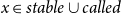 $x\in\textit{stable}\cup\textit{called}$
. Otherwise, it holds that
$x\in\textit{stable}\cup\textit{called}$
. Otherwise, it holds that
-
1. s’ is again consistent;
-
2.
$\textit{called}'=\textit{called}$
and
$\textit{stable}\subseteq\textit{stable}'$
where for all
$y\in\textit{stable}\cup\textit{called}$
,
$\sigma'\,y=\sigma\,y$
and
$\textit{infl}\,y\subseteq\textit{infl}'\,y$
; -
3.
$\textit{point}\subseteq\textit{point}'$
; -
4.
$x\in\textit{stable}'$
.


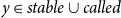


Also, each call
 $\textsf{eval}\,x\,y$
encountered during the evaluation starts in a consistent state s where
$\textsf{eval}\,x\,y$
encountered during the evaluation starts in a consistent state s where
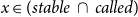 $x\in(\textit{stable}\,\cap\,\textit{called})$
. Upon its termination, a solver state s’ is attained such that
$x\in(\textit{stable}\,\cap\,\textit{called})$
. Upon its termination, a solver state s’ is attained such that
-
1. s’ is again consistent;
-
2.
$\textit{called}'=\textit{called}$
; -
3.
$\textit{stable}\subseteq\textit{stable}'$
where for all
$y'\in\textit{stable}\cup\textit{called}$
,
$\sigma'\,y'=\sigma\,y'$
and
$\textit{infl}\,y'\subseteq\textit{infl}'\,y'$
; -
4.
$\textit{point}\subseteq\textit{point}'$
; -
5. If
$y\in\textit{stable}\cup\textit{called}$
, then -
−
$\sigma' = \sigma$
,
$\textit{stable}'=\textit{stable}$
and
$\textit{point}' = \textit{point}$
if
$y\not\in\textit{called}$
whereas
$\textit{point}' = \textit{point}\cup\{y\}$
if
$y\not\in\textit{called}$
; ; -
−
$\textit{infl}'\,y'=\textit{infl}\,y'$
for all
$y'\neq y$
, and -
−
$\textit{infl}'\,y= \textit{infl}\,y\cup\{x\}$
; -
6.
$y\in\textit{stable}'$
,
$x\in\textit{infl}'\,y$
, and the value
$\sigma'\,y$
is returned.
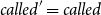


In particular, x is still contained in
 $\textit{stable}'\cap\textit{called}'$
. Finally, consider the call to
$\textit{stable}'\cap\textit{called}'$
. Finally, consider the call to
 $\textsf{destabilize}\,x$
in the body of
$\textsf{destabilize}\,x$
in the body of
 $\textsf{solve}$
, and let
$\textsf{solve}$
, and let
 $s=(\sigma,\textit{infl},\textit{stable},\textit{called},\textit{point})$
before this call. Then, s is consistent with
$s=(\sigma,\textit{infl},\textit{stable},\textit{called},\textit{point})$
before this call. Then, s is consistent with
 $x\in\textit{stable}\backslash\textit{called}$
, where upon termination of the call, a solver state s’ is attained so that
$x\in\textit{stable}\backslash\textit{called}$
, where upon termination of the call, a solver state s’ is attained so that
-
1. s’ is again consistent;
-
2.
$\sigma'=\sigma,\textit{called}=\textit{called}',\textit{point}=\textit{point}'$
; -
3.
$\textit{stable}'\subseteq\textit{stable}$
, and -
4. for all y,
$\textit{infl}'\,y$
either equals
$\unicode{x00D8}$
or
$\textit{infl}\,y$
where
$\textit{infl}'$
and
$\textit{stable}'$
are maximal so that s’ is consistent while
$\textit{infl}'\,x=\unicode{x00D8}$
and
$\textit{infl}\,x\cap\textit{stable}'=\unicode{x00D8}$
.


This invariant allows us to prove that the solver
 $\mathbf{TD}_{\mathbf{term}}$
indeed terminates for arbitrary systems of abstract equations.
$\mathbf{TD}_{\mathbf{term}}$
indeed terminates for arbitrary systems of abstract equations.
Theorem 1 Let
 $\mathbb{E}^\sharp$
denote an arbitrary system of abstract equations, and let
$\mathbb{E}^\sharp$
denote an arbitrary system of abstract equations, and let
 $x_0$
be the initial unknown of interest. Assume that initially the sets
$x_0$
be the initial unknown of interest. Assume that initially the sets
 $\textit{called}$
and
$\textit{called}$
and
 $\textit{stable}$
are empty, and likewise,
$\textit{stable}$
are empty, and likewise,
 $\textit{infl}$
maps each unknown to the empty set. Then, the call
$\textit{infl}$
maps each unknown to the empty set. Then, the call
 $\textsf{solve}\,\nabla\,x_0$
will always terminate, as long as only finitely many unknowns are encountered.
$\textsf{solve}\,\nabla\,x_0$
will always terminate, as long as only finitely many unknowns are encountered.
Proof. First we note that every call
 $\textsf{destabilize}\,y$
terminates. This is immediate in case when
$\textsf{destabilize}\,y$
terminates. This is immediate in case when
 $\textit{infl}\,y$
is empty. Moreover,
$\textit{infl}\,y$
is empty. Moreover,
 $\textit{infl}\,y'$
is non-empty for only finitely many unknowns y’. Since the set
$\textit{infl}\,y'$
is non-empty for only finitely many unknowns y’. Since the set
 $\textit{infl}\,y$
is set to
$\textit{infl}\,y$
is set to
 $\unicode{x00D8}$
, before any recursive call to unknowns, termination follows.
$\unicode{x00D8}$
, before any recursive call to unknowns, termination follows.
Assume now that during evaluation of the initial call
 $\textsf{solve}\,\nabla\,x_0$
, only finitely many unknowns x are encountered for which
$\textsf{solve}\,\nabla\,x_0$
, only finitely many unknowns x are encountered for which
 $\textsf{solve}\;p\;x$
is called for some p.
$\textsf{solve}\;p\;x$
is called for some p.
In order to prove termination of all calls
 $\textsf{solve}\,p\,x$
encountered during the evaluation of
$\textsf{solve}\,p\,x$
encountered during the evaluation of
 $\textsf{solve}\,\nabla\,x_0$
, we perform an induction on the cardinality of the set of unknowns which are not in
$\textsf{solve}\,\nabla\,x_0$
, we perform an induction on the cardinality of the set of unknowns which are not in
 $\textit{called}$
. Let Y denote the set of all unknowns
$\textit{called}$
. Let Y denote the set of all unknowns
 $y\in\mathcal{X}\setminus(\{x\}\cup\textit{called}\cup\textit{stable})$
for which
$y\in\mathcal{X}\setminus(\{x\}\cup\textit{called}\cup\textit{stable})$
for which
 $\textsf{solve}\,\nabla\,y$
is called during the call
$\textsf{solve}\,\nabla\,y$
is called during the call
 $\textsf{solve}\,p\,x$
and proceeds to the evaluation of the right-hand side of y.
$\textsf{solve}\,p\,x$
and proceeds to the evaluation of the right-hand side of y.
Assume for a contradiction that the call
 $\textsf{solve}\,p\,x$
would not terminate. Let us first assume that
$\textsf{solve}\,p\,x$
would not terminate. Let us first assume that
 $x\not\in\textit{point}$
throughout the iteration, that is, all tail-recursive calls to
$x\not\in\textit{point}$
throughout the iteration, that is, all tail-recursive calls to
 $\textsf{solve}\,p\,x$
. In particular, this means that for none of the unknowns
$\textsf{solve}\,p\,x$
. In particular, this means that for none of the unknowns
 $y\in Y$
, evaluation of the right-hand side
$y\in Y$
, evaluation of the right-hand side
 $f^\sharp{}_y$
accessed the unknown x – as in this case, x would have been added to
$f^\sharp{}_y$
accessed the unknown x – as in this case, x would have been added to
 $\textit{point}$
. Therefore, when
$\textit{point}$
. Therefore, when
 $p = \nabla$
,
$p = \nabla$
,
 $\textit{infl}\,x$
does not contain any of the unknowns in Y, that is, is still empty after the first update of
$\textit{infl}\,x$
does not contain any of the unknowns in Y, that is, is still empty after the first update of
 $\sigma\,x$
. Accordingly, destabilization of x will immediately terminate and leave x in the set
$\sigma\,x$
. Accordingly, destabilization of x will immediately terminate and leave x in the set
 $\textit{stable}$
. If
$\textit{stable}$
. If
 $p = \Delta$
,
$p = \Delta$
,
 $\textit{infl}\,x = \unicode{x00D8}$
at least for all calls after the first call to
$\textit{infl}\,x = \unicode{x00D8}$
at least for all calls after the first call to
 $\textsf{solve}\,\Delta\,x$
. As a consequence, the call
$\textsf{solve}\,\Delta\,x$
. As a consequence, the call
 $\textsf{solve}\,p\,x$
terminates for each phase p – in contradiction to our assumption.
$\textsf{solve}\,p\,x$
terminates for each phase p – in contradiction to our assumption.
Therefore, necessarily,
 $x\in\textit{point}$
at least after the first evaluation of
$x\in\textit{point}$
at least after the first evaluation of
 $f^\sharp{}_{x}$
. We distinguish two cases.
$f^\sharp{}_{x}$
. We distinguish two cases.
Case 1.
 $p=\Delta$
.
$p=\Delta$
.
By inductive hypothesis, all occurring calls
 $\textsf{solve}\,p\,y$
with
$\textsf{solve}\,p\,y$
with
 $y\in Y$
terminate. Let
$y\in Y$
terminate. Let
 $a_i,i\geq 0$
denote the sequence of values of
$a_i,i\geq 0$
denote the sequence of values of
 $\sigma\,x$
before the ith tail-recursive call to
$\sigma\,x$
before the ith tail-recursive call to
 $\textsf{solve}\,\Delta\,x$
. Then necessarily
$\textsf{solve}\,\Delta\,x$
. Then necessarily
 $a_i\neq a_{i+1}$
for all
$a_i\neq a_{i+1}$
for all
 $i\geq 0$
. Let
$i\geq 0$
. Let
 $b_1,\ldots,b_i,\ldots$
denote the sequence of values returned by the ith evaluation of the right-hand side
$b_1,\ldots,b_i,\ldots$
denote the sequence of values returned by the ith evaluation of the right-hand side
 $f^\sharp{}_{x}$
of x. Then,
$f^\sharp{}_{x}$
of x. Then,
 $a_{i+1} = a_i\Delta b_{i+1}$
for
$a_{i+1} = a_i\Delta b_{i+1}$
for
 $i\geq 0$
. Due to the properties of narrowing, however, the latter sequence is ultimately stable, that is,
$i\geq 0$
. Due to the properties of narrowing, however, the latter sequence is ultimately stable, that is,
 $a_i= a_{i+1}$
for some i – in which case the recursion terminates: contradiction. Therefore, each call
$a_i= a_{i+1}$
for some i – in which case the recursion terminates: contradiction. Therefore, each call
 $\textsf{solve}\,\Delta\,x$
eventually terminates.
$\textsf{solve}\,\Delta\,x$
eventually terminates.
Case 2.
 $p=\nabla$
.
$p=\nabla$
.
By inductive hypothesis, again all calls
 $\textsf{solve}\,\nabla\,y$
with
$\textsf{solve}\,\nabla\,y$
with
 $y\in Y$
terminate. Let
$y\in Y$
terminate. Let
 $a_i,i\geq 0$
denote the sequence of values of
$a_i,i\geq 0$
denote the sequence of values of
 $\sigma\,x$
before the ith tail-recursive call to
$\sigma\,x$
before the ith tail-recursive call to
 $\textsf{solve}\,\nabla\,x$
. Assume that
$\textsf{solve}\,\nabla\,x$
. Assume that
 $a_i\neq a_{i+1}$
for all
$a_i\neq a_{i+1}$
for all
 $i\geq 0$
. Let
$i\geq 0$
. Let
 $b_1,\ldots$
denote the sequence of values returned by the ith evaluation of the right-hand side
$b_1,\ldots$
denote the sequence of values returned by the ith evaluation of the right-hand side
 $f^\sharp{}_x$
of x. Then,
$f^\sharp{}_x$
of x. Then,
 $a_{i+1} = a_i\nabla b_{i+1}$
for
$a_{i+1} = a_i\nabla b_{i+1}$
for
 $i\geq 0$
. Due to the properties of widening, however, the latter sequence is ultimately stable, that is,
$i\geq 0$
. Due to the properties of widening, however, the latter sequence is ultimately stable, that is,
 $a_i= a_{i+1}$
for some i. Therefore eventually,
$a_i= a_{i+1}$
for some i. Therefore eventually,
 $\textsf{solve}\,\Delta\,x$
is tail-recursively called. But then, termination follows due to termination of the call
$\textsf{solve}\,\Delta\,x$
is tail-recursively called. But then, termination follows due to termination of the call
 $\textsf{solve}\,\Delta\,x$
: contradiction!
$\textsf{solve}\,\Delta\,x$
: contradiction!
Accordingly, we conclude that all encountered calls
 $\textsf{solve}\,p\,x$
terminate, and thus also the call
$\textsf{solve}\,p\,x$
terminate, and thus also the call
 $\textsf{solve}\,\nabla\,x_0$
.
$\textsf{solve}\,\nabla\,x_0$
.
6. Correctness of TDterm
Our goal is to prove that the result of our algorithm is a sound description of the least partial solution of the concrete system. In case of monotonic abstract systems and total solutions, soundness is known to hold for any post-solution of the abstract system, whenever the concrete system is described by the abstract system. Recall that while the right-hand sides of our concrete system are monotonic, this need not necessarily be the case for the abstract system. Consider, for example, an interprocedural analysis as in Examples 5 and 6 and there the elaborated right-hand side
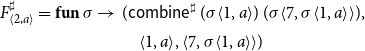 \begin{equation*}F^\sharp_{{\langle2,a\rangle}} =\textbf{fun}\,\sigma\to \begin{array}[t]{l} (\textsf{combine}^\sharp\,(\sigma{\langle1,a\rangle})\,(\sigma{\langle7,\sigma{\langle1,a\rangle}\rangle}),\\ \quad{{\langle1,a\rangle},{\langle7,\sigma{\langle1,a\rangle}\rangle}}) \end{array}\end{equation*}
for the unknown
 ${\langle2,a\rangle}$
. Since for different values in
${\langle2,a\rangle}$
. Since for different values in
 $\sigma$
for
$\sigma$
for
 ${\langle1,a\rangle}$
, different unknowns are queried, this function cannot be monotonic. In order to deal with such non-monotonicities, Frielinghaus et al. (Reference Frielinghaus, Seidl and Vogler2016) have introduced the concept of a lower monotonization of the abstract system
${\langle1,a\rangle}$
, different unknowns are queried, this function cannot be monotonic. In order to deal with such non-monotonicities, Frielinghaus et al. (Reference Frielinghaus, Seidl and Vogler2016) have introduced the concept of a lower monotonization of the abstract system
 $\mathbb{E}^\sharp$
.
$\mathbb{E}^\sharp$
.
For the system
 $\mathbb{E}^\sharp$
with set of unknowns
$\mathbb{E}^\sharp$
with set of unknowns
 $\mathcal{X}^\sharp$
, the lower monotonization
$\mathcal{X}^\sharp$
, the lower monotonization
 $\underline{\mathbb{E}^\sharp}$
is a system of equations with the same set of unknowns where the elaborated right-hand side
$\underline{\mathbb{E}^\sharp}$
is a system of equations with the same set of unknowns where the elaborated right-hand side
 $\underline{F}_{x}^\sharp$
for
$\underline{F}_{x}^\sharp$
for
 $x\in\mathcal{X}^\sharp$
is given by
$x\in\mathcal{X}^\sharp$
is given by
 $\underline{F}_{x}^\sharp\,\sigma = (d,X)$
with
$\underline{F}_{x}^\sharp\,\sigma = (d,X)$
with
 \begin{equation*}\begin{array}{lll} d &=& \sqcap{(F^\sharp{}_{x}\,\sigma')_1\mid \sigma'\sqsupseteq\sigma} \\ X &=& \mathcal{X}^\sharp \\\end{array}\end{equation*}
Thus, we over-approximate the sets of unknowns influencing the result of a right-hand side by the full set
 $\mathcal{X}^\sharp$
while d is the greatest lower bound to all first components of results of
$\mathcal{X}^\sharp$
while d is the greatest lower bound to all first components of results of
 $F^\sharp{}_x$
for assignments exceeding
$F^\sharp{}_x$
for assignments exceeding
 $\sigma$
.
$\sigma$
.
Since all right-hand sides of
 $\underline{\mathbb{E}^\sharp}$
are monotonic, the system has a least total solution
$\underline{\mathbb{E}^\sharp}$
are monotonic, the system has a least total solution
 $\underline\sigma$
. Let
$\underline\sigma$
. Let
 $\sigma$
denote the least total solution of some concrete system
$\sigma$
denote the least total solution of some concrete system
 $\mathbb{E}$
which is described by
$\mathbb{E}$
which is described by
 $\mathbb{E}^\sharp$
. In Frielinghaus et al. (Reference Frielinghaus, Seidl and Vogler2016), it has been proven that then also
$\mathbb{E}^\sharp$
. In Frielinghaus et al. (Reference Frielinghaus, Seidl and Vogler2016), it has been proven that then also
 $\sigma\mathrel{\mathcal{R}}\underline\sigma$
holds. Moreover, let
$\sigma\mathrel{\mathcal{R}}\underline\sigma$
holds. Moreover, let
 $\textit{dom}$
denote the least
$\textit{dom}$
denote the least
 $(\sigma,\mathbb{E})$
-closed subset containing some initial unknown x. Let
$(\sigma,\mathbb{E})$
-closed subset containing some initial unknown x. Let
 $x\mathrel{\mathcal{R}} y$
for some unknown
$x\mathrel{\mathcal{R}} y$
for some unknown
 $y\in\mathcal{X}^\sharp$
. Let
$y\in\mathcal{X}^\sharp$
. Let
 $\sigma':\mathcal{X}^\sharp\to\mathbb{D}$
be some abstract assignment, and
$\sigma':\mathcal{X}^\sharp\to\mathbb{D}$
be some abstract assignment, and
 $\textit{dom}^\sharp$
be
$\textit{dom}^\sharp$
be
 $(\sigma',\mathbb{E}^\sharp)$
-closed with
$(\sigma',\mathbb{E}^\sharp)$
-closed with
 $y\in\textit{dom}^\sharp$
. Assume further that
$y\in\textit{dom}^\sharp$
. Assume further that
 $\underline\sigma\,y'\sqsubseteq\sigma'\,y'$
for all
$\underline\sigma\,y'\sqsubseteq\sigma'\,y'$
for all
 $y'\in\textit{dom}^\sharp$
. Then by the results of Frielinghaus et al. (Reference Frielinghaus, Seidl and Vogler2016), also
$y'\in\textit{dom}^\sharp$
. Then by the results of Frielinghaus et al. (Reference Frielinghaus, Seidl and Vogler2016), also
 $\textit{dom}\mathrel{\mathcal{R}}\textit{dom}^\sharp$
holds. Accordingly, the pair
$\textit{dom}\mathrel{\mathcal{R}}\textit{dom}^\sharp$
holds. Accordingly, the pair
 $(\sigma',\textit{dom}^\sharp)$
can then be understood as a sound description of the least partial post-solution of the concrete system
$(\sigma',\textit{dom}^\sharp)$
can then be understood as a sound description of the least partial post-solution of the concrete system
 $\mathbb{E}$
for x.
$\mathbb{E}$
for x.
Therefore, now assume that we are given a set X of unknowns of the concrete system of equations
 $\mathbb{E}$
, together with a an abstract unknown
$\mathbb{E}$
, together with a an abstract unknown
 $x_0$
so that for all
$x_0$
so that for all
 $x\in X$
,
$x\in X$
,
 $x\mathrel{\mathcal{R}} x_0$
holds. Assume further that the solver
$x\mathrel{\mathcal{R}} x_0$
holds. Assume further that the solver
 $\mathbf{TD}_{\mathbf{term}}$
, when started with the call
$\mathbf{TD}_{\mathbf{term}}$
, when started with the call
 $\textsf{solve}\,\nabla\,x_0$
, returns the abstract assignment
$\textsf{solve}\,\nabla\,x_0$
, returns the abstract assignment
 $\sigma^\sharp$
where by default,
$\sigma^\sharp$
where by default,
 $\sigma^\sharp\,y=\bot$
for all unknowns y which have not been encountered during solving. It therefore suffices to prove:
$\sigma^\sharp\,y=\bot$
for all unknowns y which have not been encountered during solving. It therefore suffices to prove:
-
1. There is a subset
$\textit{dom}^\sharp\subseteq\mathcal{X}^\sharp$
containing
$x_0$
which is
$(\sigma^\sharp,\mathbb{E}^\sharp)$
-closed. -
2.
$\underline\sigma^\sharp\,y\sqsubseteq\sigma^\sharp\,y$
holds for all
$y\in\textit{dom}^\sharp$
.


After evaluation of each call
 $\textsf{solve}\,p\,x$
, evaluation of the right-hand side of an unknown in stable will access only unknowns which are either again in stable, or in called. As a consequence, the set of all stable unknowns after termination of all calls
$\textsf{solve}\,p\,x$
, evaluation of the right-hand side of an unknown in stable will access only unknowns which are either again in stable, or in called. As a consequence, the set of all stable unknowns after termination of all calls
 $\textsf{solve}\,\nabla\,x_0$
is
$\textsf{solve}\,\nabla\,x_0$
is
 $(\sigma^\sharp,\mathbb{E}^\sharp)$
-closed. Therefore, it remains to verify the second property. Let
$(\sigma^\sharp,\mathbb{E}^\sharp)$
-closed. Therefore, it remains to verify the second property. Let
 $\textit{dom}^\sharp$
denote the subset
$\textit{dom}^\sharp$
denote the subset
 $\textit{stable}\subseteq\mathcal{X}^\sharp$
upon termination of the call
$\textit{stable}\subseteq\mathcal{X}^\sharp$
upon termination of the call
 $\textsf{solve}\,\nabla\,x_0$
. Let
$\textsf{solve}\,\nabla\,x_0$
. Let
 $\underline\sigma : \mathcal{X}^\sharp\to\mathbb{D}$
denote the least solution of the lower monotonization
$\underline\sigma : \mathcal{X}^\sharp\to\mathbb{D}$
denote the least solution of the lower monotonization
 $\underline{\mathbb{E}^\sharp}$
of
$\underline{\mathbb{E}^\sharp}$
of
 $\mathbb{E}^\sharp$
. Our goal is to show that
$\mathbb{E}^\sharp$
. Our goal is to show that
 $\underline\sigma\,x\sqsubseteq\sigma^\sharp\,x$
for all
$\underline\sigma\,x\sqsubseteq\sigma^\sharp\,x$
for all
 $x\in\textit{dom}^\sharp$
.
$x\in\textit{dom}^\sharp$
.
Assume that we are given a subset Y of unknowns together with an assignment
 $\tau : Y\to\mathbb{D}$
. Here, we assume Y and
$\tau : Y\to\mathbb{D}$
. Here, we assume Y and
 $\tau$
to represent the set of unknowns which are currently stable (or called) together with their current values. In the following, we use the binary operator
$\tau$
to represent the set of unknowns which are currently stable (or called) together with their current values. In the following, we use the binary operator
 $\oplus$
to denote an update of the left argument with the bindings provided by the right argument. Let
$\oplus$
to denote an update of the left argument with the bindings provided by the right argument. Let
 $\mathbb{E}^\sharp{}_{\tau}$
denote the system of equations with unknowns from
$\mathbb{E}^\sharp{}_{\tau}$
denote the system of equations with unknowns from
 $\mathcal{X}^\sharp\setminus Y$
where the right-hand side
$\mathcal{X}^\sharp\setminus Y$
where the right-hand side
 $f^\sharp_{\tau,y}$
of y behaves like the right-hand side
$f^\sharp_{\tau,y}$
of y behaves like the right-hand side
 $f^\sharp{}_y$
of
$f^\sharp{}_y$
of
 $\mathbb{E}^\sharp$
, but looks up the values for encountered unknowns from Y in
$\mathbb{E}^\sharp$
, but looks up the values for encountered unknowns from Y in
 $\tau$
. Technically, this means that
$\tau$
. Technically, this means that
 \begin{equation*}\begin{array}{lll}f^\sharp{}_{\tau,y}\,\sigma &=& f^\sharp{}_y\,(\sigma\oplus(\textsf{return}\circ\tau))\end{array}\end{equation*}
Accordingly, the elaborated right-hand side
 $F^\sharp{}_{\tau,y}$
for the unknown y is given by
$F^\sharp{}_{\tau,y}$
for the unknown y is given by
 \begin{equation*}F^\sharp{}_{\tau,y}\,\sigma \quad=\begin{array}[t]{l} \textbf{let}\; (d,X) = F^\sharp{}_{y}\,(\sigma\oplus\tau)\\ \textbf{in}\; (d,X\setminus Y) \end{array}\end{equation*}
Let
 $s=(\sigma,\textit{infl},\textit{stable},\textit{called},\textit{point})$
denote a consistent solver state. Let
$s=(\sigma,\textit{infl},\textit{stable},\textit{called},\textit{point})$
denote a consistent solver state. Let
 $\tau : \textit{called}\to\mathbb{D}$
denote the restriction of
$\tau : \textit{called}\to\mathbb{D}$
denote the restriction of
 $\sigma$
to the set
$\sigma$
to the set
 $\textit{called}$
. We call s saturated if for all
$\textit{called}$
. We call s saturated if for all
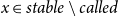 $x\in \textit{stable}\setminus\textit{called}$
,
$x\in \textit{stable}\setminus\textit{called}$
,
 $\underline\sigma\, x \sqsubseteq \sigma\,x$
where
$\underline\sigma\, x \sqsubseteq \sigma\,x$
where
 $(\underline\sigma,X^\sharp\setminus\textit{called})$
is the least total solution of the lower monotonization of
$(\underline\sigma,X^\sharp\setminus\textit{called})$
is the least total solution of the lower monotonization of
 $\mathbb{E}^\sharp{}_\tau$
. We claim:
$\mathbb{E}^\sharp{}_\tau$
. We claim:
Theorem 2. Each call
 $\textsf{solve}\,\nabla\,x$
starting in a saturated solver state, results upon termination, in a solver state
$\textsf{solve}\,\nabla\,x$
starting in a saturated solver state, results upon termination, in a solver state
 $s'=(\sigma',\textit{infl}',\textit{stable}',\textit{called}',\textit{point}')$
which is again saturated where additionally,
$s'=(\sigma',\textit{infl}',\textit{stable}',\textit{called}',\textit{point}')$
which is again saturated where additionally,
 $x\in\textit{stable}'$
. Since before the initial call
$x\in\textit{stable}'$
. Since before the initial call
 $\textsf{solve}\,\nabla\,x_0$
the set
$\textsf{solve}\,\nabla\,x_0$
the set
 $\textit{called}$
is empty, this theorem implies that upon termination,
$\textit{called}$
is empty, this theorem implies that upon termination,
 $\textit{dom}^\sharp$
is
$\textit{dom}^\sharp$
is
 $(\sigma',\mathbb{E}^\sharp)$
-closed with
$(\sigma',\mathbb{E}^\sharp)$
-closed with
 $x_0\in\textit{dom}^\sharp$
, and
$x_0\in\textit{dom}^\sharp$
, and
 $\underline\sigma\,x\sqsubseteq\sigma'\,x$
for all
$\underline\sigma\,x\sqsubseteq\sigma'\,x$
for all
 $x\in\textit{dom}^\sharp$
.
$x\in\textit{dom}^\sharp$
.
Proof. We proceed by induction on the set
 $\mathcal{X}'$
of unknowns not contained in the set
$\mathcal{X}'$
of unknowns not contained in the set
 $\textit{stable}$
of stable unknowns before the call. For
$\textit{stable}$
of stable unknowns before the call. For
 $\mathcal{X}'=\unicode{x00D8}$
, the assertion obviously holds. For the inductive step, first assume that after the evaluation of the right-hand side
$\mathcal{X}'=\unicode{x00D8}$
, the assertion obviously holds. For the inductive step, first assume that after the evaluation of the right-hand side
 $f^\sharp{}_{x}$
, x is not included in
$f^\sharp{}_{x}$
, x is not included in
 $\textit{point}$
. This means that no variable in
$\textit{point}$
. This means that no variable in
 $\mathcal{X}'$
may depend on the unknown x. Assume that the values of x before and after
$\mathcal{X}'$
may depend on the unknown x. Assume that the values of x before and after
 $\textsf{solve}$
are d and d’, respectively. Consider the least total solutions
$\textsf{solve}$
are d and d’, respectively. Consider the least total solutions
 $\underline\sigma$
and
$\underline\sigma$
and
 $\underline\sigma'$
of the lower monotonizations of the systems
$\underline\sigma'$
of the lower monotonizations of the systems
 $\mathbb{E}^\sharp{}_{\tau}$
and
$\mathbb{E}^\sharp{}_{\tau}$
and
 $\mathbb{E}^\sharp{}_{\tau\oplus\{x\mapsto d'\}}$
, respectively, where
$\mathbb{E}^\sharp{}_{\tau\oplus\{x\mapsto d'\}}$
, respectively, where
 $\tau : \textit{stable}\to\mathbb{D}$
records the values of all unknowns from
$\tau : \textit{stable}\to\mathbb{D}$
records the values of all unknowns from
 $\textit{stable}$
. Let
$\textit{stable}$
. Let
 $Y = (F^\sharp{}_{\tau\oplus\{x\mapsto d\},x})_2\setminus\textit{stable}$
be the set of unknowns accessed during the evaluation of the right-hand side for x (in particular,
$Y = (F^\sharp{}_{\tau\oplus\{x\mapsto d\},x})_2\setminus\textit{stable}$
be the set of unknowns accessed during the evaluation of the right-hand side for x (in particular,
 $x\not\in Y$
). Then
$x\not\in Y$
). Then
 $\mathcal{X}'\setminus\{x\}$
is the disjoint union of subsets
$\mathcal{X}'\setminus\{x\}$
is the disjoint union of subsets
 $\mathcal{X}'_y,y\in Y$
, where
$\mathcal{X}'_y,y\in Y$
, where
 $\mathcal{X}'_y$
is the subset of unknowns freshly solved when y is encountered. By applying the inductive hypothesis to the unknowns in y in sequence, we obtain that for all
$\mathcal{X}'_y$
is the subset of unknowns freshly solved when y is encountered. By applying the inductive hypothesis to the unknowns in y in sequence, we obtain that for all
 $y\in Y$
,
$y\in Y$
,
 $\underline\sigma'\,y'\sqsubseteq\sigma\,y'$
for all
$\underline\sigma'\,y'\sqsubseteq\sigma\,y'$
for all
 $y'\in\mathcal{X}{}_y$
. Accordingly, we have for all
$y'\in\mathcal{X}{}_y$
. Accordingly, we have for all
 $y\in\mathcal{X}'\setminus\{x\}$
, that
$y\in\mathcal{X}'\setminus\{x\}$
, that
 \begin{equation*}(\underline F'_y\underline\sigma')_1\sqsubseteq\sigma'\,y\end{equation*}
Here,
 $\underline F'_{y}$
denotes the elaborated right-hand side of the lower monotonization of
$\underline F'_{y}$
denotes the elaborated right-hand side of the lower monotonization of
 $\mathbb{E}{}_{\tau\oplus\{x\mapsto d'\}}$
for y. This allows us to deduce for x that
$\mathbb{E}{}_{\tau\oplus\{x\mapsto d'\}}$
for y. This allows us to deduce for x that
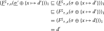 \begin{equation*}\begin{array}{lll}(\underline F^\sharp{}_{\tau,x}(\underline\sigma'\oplus\{x\mapsto d'\}))_1&\sqsubseteq &(\underline F^\sharp{}_{\tau,x}(\sigma\oplus\{x\mapsto d'\}))_1 \\&\sqsubseteq& (F^\sharp{}_{\tau,x}(\sigma\oplus\{x\mapsto d'\}))_1 \\&=& (F^\sharp{}_{\tau,x}(\sigma\oplus\{x\mapsto d\}))_1 \\&=& d'\end{array}\end{equation*}
Thereby, we have used that the value of the unknown x is not contained in
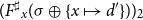 $(F^\sharp{}_{x}(\sigma\oplus\{x\mapsto d'\}))_2$
– implying that it is also not contained in
$(F^\sharp{}_{x}(\sigma\oplus\{x\mapsto d'\}))_2$
– implying that it is also not contained in
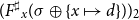 $(F^\sharp{}_{x}(\sigma\oplus\{x\mapsto d\}))_2$
. Moreover, for
$(F^\sharp{}_{x}(\sigma\oplus\{x\mapsto d\}))_2$
. Moreover, for
 $y\in\mathcal{X}'$
different from x,
$y\in\mathcal{X}'$
different from x,
 \begin{equation*}(\underline F^\sharp{}_{\tau,y}\,(\underline\sigma'\oplus\{x\mapsto d'\}))_1 \sqsubseteq(\underline F'_{y}\,\underline\sigma')_1\sqsubseteq\underline\sigma'\,y\end{equation*}
Accordingly,
 $\underline\sigma'\oplus\{x\mapsto d'\}$
is a post-solution of the lower monotonization of
$\underline\sigma'\oplus\{x\mapsto d'\}$
is a post-solution of the lower monotonization of
 $\mathbb{E}{}_\tau$
, implying that
$\mathbb{E}{}_\tau$
, implying that
 $\underline\sigma\sqsubseteq\sigma'$
.
$\underline\sigma\sqsubseteq\sigma'$
.
Now assume that after the evaluation of the right-hand side
 $f^\sharp{}_{x}$
,
$f^\sharp{}_{x}$
,
 $x\in\textit{point}$
holds. We concentrate on the last tail-recursive call
$x\in\textit{point}$
holds. We concentrate on the last tail-recursive call
 $\textsf{solve}\,\nabla\,x$
before the call to
$\textsf{solve}\,\nabla\,x$
before the call to
 $\textsf{solve}\,\Delta\,x$
. Let
$\textsf{solve}\,\Delta\,x$
. Let
 $s_0 = (\sigma{}_0,\textit{infl}{}_0,\textit{stable}{}_0,\textit{called}{}_0,\textit{point}{}_0)$
. Let d denote the value of x before the evaluation of the right-hand side, and d’ the value returned by evaluating the right-hand side. Let
$s_0 = (\sigma{}_0,\textit{infl}{}_0,\textit{stable}{}_0,\textit{called}{}_0,\textit{point}{}_0)$
. Let d denote the value of x before the evaluation of the right-hand side, and d’ the value returned by evaluating the right-hand side. Let
 $\mathcal{X}'$
denote the set of unknowns accessed during the call which are not stable before. Since subsequently
$\mathcal{X}'$
denote the set of unknowns accessed during the call which are not stable before. Since subsequently
 $\textsf{solve}\,\Delta\,x$
is called, after that the evaluation of
$\textsf{solve}\,\Delta\,x$
is called, after that the evaluation of
 $f^\sharp_{x}$
, x is still stable. Therefore, one of the following two situations is encountered after the evaluation of the right-hand side:
$f^\sharp_{x}$
, x is still stable. Therefore, one of the following two situations is encountered after the evaluation of the right-hand side:
-
1.
$d'\sqsubseteq d$
, that is, the value d’ is subsumed by the current value of x; or -
2. subsequent destabilization will not destabilize x.

In the second case, the unknowns from
 $\mathcal{X}'$
that directly or indirectly influence x cannot depend on x (w.r.t. the current map
$\mathcal{X}'$
that directly or indirectly influence x cannot depend on x (w.r.t. the current map
 $\textit{infl}$
). Thus, a similar argument as for unknowns not in
$\textit{infl}$
). Thus, a similar argument as for unknowns not in
 $\textit{point}$
applies.
$\textit{point}$
applies.
Accordingly, it remains to consider the first case. Consider the lower monotonizations of the abstract systems
 $\mathbb{E}^\sharp{}_\tau$
and
$\mathbb{E}^\sharp{}_\tau$
and
 $\mathbb{E}^\sharp{}_{\tau\oplus\{x\mapsto d\}}$
with least solutions
$\mathbb{E}^\sharp{}_{\tau\oplus\{x\mapsto d\}}$
with least solutions
 $\underline\sigma$
and
$\underline\sigma$
and
 $\underline\sigma'$
, respectively. By inductive hypothesis applied to the unknowns in
$\underline\sigma'$
, respectively. By inductive hypothesis applied to the unknowns in
 $\mathcal{X}'\setminus\{x\}$
and
$\mathcal{X}'\setminus\{x\}$
and
 $\tau\oplus\{x\mapsto d\}$
, we find that
$\tau\oplus\{x\mapsto d\}$
, we find that
 $\underline\sigma'\,y\sqsubseteq\sigma{}_0\,y$
for all unknowns
$\underline\sigma'\,y\sqsubseteq\sigma{}_0\,y$
for all unknowns
 $y\in\mathcal{X}'\setminus\{x\}$
. This allows us to prove that
$y\in\mathcal{X}'\setminus\{x\}$
. This allows us to prove that
 $\underline\sigma'\oplus\{x\mapsto d\}$
is a post-solution of the lower monotonization of
$\underline\sigma'\oplus\{x\mapsto d\}$
is a post-solution of the lower monotonization of
 $\mathbb{E}^\sharp{}_\tau$
. Therefore,
$\mathbb{E}^\sharp{}_\tau$
. Therefore,
 $\underline\sigma\,y \sqsubseteq(\underline\sigma'\oplus\{x\mapsto d\})\,y \sqsubseteq(\sigma{}_0\oplus\{x\mapsto d\})\,y$
for all
$\underline\sigma\,y \sqsubseteq(\underline\sigma'\oplus\{x\mapsto d\})\,y \sqsubseteq(\sigma{}_0\oplus\{x\mapsto d\})\,y$
for all
 $y\in\mathcal{X}'$
holds, and the claim follows.
$y\in\mathcal{X}'$
holds, and the claim follows.
Now consider the narrowing iteration performed for x in the subsequent call
 $\textsf{solve}\,\Delta\,x$
. Let
$\textsf{solve}\,\Delta\,x$
. Let
 $d_0$
denote the value after the last call to
$d_0$
denote the value after the last call to
 $\textsf{solve}\,\nabla\,x$
, and
$\textsf{solve}\,\nabla\,x$
, and
 $d_1,\ldots, d_k$
denote the values returned by evaluating the right-hand side of x during this iteration and define
$d_1,\ldots, d_k$
denote the values returned by evaluating the right-hand side of x during this iteration and define
 $d'_0 = d_0$
and for
$d'_0 = d_0$
and for
 $i>0$
,
$i>0$
,
 $d'_i = d'_{i-1}\Delta d_i$
. Let
$d'_i = d'_{i-1}\Delta d_i$
. Let
 $\sigma{}_i$
denote the assignment attained after the ith narrowing step restricted to the unknowns
$\sigma{}_i$
denote the assignment attained after the ith narrowing step restricted to the unknowns
 $\mathcal{X}^\sharp\setminus(\mathcal{X}{}_0\cup\{x\})$
. For
$\mathcal{X}^\sharp\setminus(\mathcal{X}{}_0\cup\{x\})$
. For
 $i>0$
, let
$i>0$
, let
 $\underline\sigma{}_i$
denote the least solution of the lower monotonization of
$\underline\sigma{}_i$
denote the least solution of the lower monotonization of
 $\mathbb{E}^\sharp{}_{\tau\oplus\{x\mapsto d_{i-1}\}}$
. By inductive hypothesis,
$\mathbb{E}^\sharp{}_{\tau\oplus\{x\mapsto d_{i-1}\}}$
. By inductive hypothesis,
 $\underline\sigma{}_i\,y\sqsubseteq\sigma{}_i$
for all
$\underline\sigma{}_i\,y\sqsubseteq\sigma{}_i$
for all
 $y\neq x$
which are stable after the ith iteration. By induction on i, we prove that
$y\neq x$
which are stable after the ith iteration. By induction on i, we prove that
 $\underline\sigma\,x\sqsubseteq d_i$
and thus also
$\underline\sigma\,x\sqsubseteq d_i$
and thus also
 $\underline\sigma\,x\sqsubseteq d'_i$
, and
$\underline\sigma\,x\sqsubseteq d'_i$
, and
 $\underline\sigma\,y\sqsubseteq\sigma{}_i\,y$
for every
$\underline\sigma\,y\sqsubseteq\sigma{}_i\,y$
for every
 $y\in\mathcal{X}^\sharp\setminus(\mathcal{X}{}_0\cup\{x\})$
which is stable after the ith narrowing iteration. This assertion holds for
$y\in\mathcal{X}^\sharp\setminus(\mathcal{X}{}_0\cup\{x\})$
which is stable after the ith narrowing iteration. This assertion holds for
 $i=0$
. For
$i=0$
. For
 $i>0$
, the assertion on the
$i>0$
, the assertion on the
 $y\neq x$
follows by inductive hypothesis for a larger set of called unknowns. And for x, we have
$y\neq x$
follows by inductive hypothesis for a larger set of called unknowns. And for x, we have
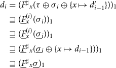 \begin{equation*}\begin{array}{lcl}d_i &=& (F^\sharp{}_{x} (\tau\oplus\sigma{}_i\oplus\{x\mapsto d'_{i-1}\}))_1 \\ &\sqsupseteq& (\underline F^{(i)}_{x}(\sigma{}_i))_1 \\ &\sqsupseteq& (\underline F^{(i)}_{x}(\underline\sigma{}_i))_1 \\ &\sqsupseteq& (\underline F^\sharp{}_{x}(\underline\sigma{}_i\oplus\{x\mapsto d_{i-1}\}))_1 \\ &\sqsupseteq& (\underline F^\sharp{}_{x}\underline\sigma)_1\end{array}\end{equation*}
Here,
 $\underline F^\sharp{}_{x}$
and
$\underline F^\sharp{}_{x}$
and
 $\underline F^{(i)}_{x}$
are the right-hand sides of the lower monotonizations of
$\underline F^{(i)}_{x}$
are the right-hand sides of the lower monotonizations of
 $\mathbb{E}^\sharp{}_\tau$
and
$\mathbb{E}^\sharp{}_\tau$
and
 $\mathbb{E}^\sharp{}_{\tau\oplus\{x\mapsto d_{i-1}\}}$
for x, respectively. This completes the proof of the theorem.
$\mathbb{E}^\sharp{}_{\tau\oplus\{x\mapsto d_{i-1}\}}$
for x, respectively. This completes the proof of the theorem.
7. The Space-efficient Solver TDspace
So far, our solver maintains an abstract value for each queried unknown. Given that the program to be analyzed is not small (e.g., more than 10,000 LOC) and program points must be analyzed for multiple contexts, the number of unknowns to be considered by the solver can be quite large. For more complicated properties to be analyzed, these abstract values to be recorded for these unknowns in themselves are space-consuming. The applicability of solvers for interprocedural analysis based on such solvers therefore is significantly increased if space consumption can be reduced. This is the objective of our second modification to the local generic solver TD.

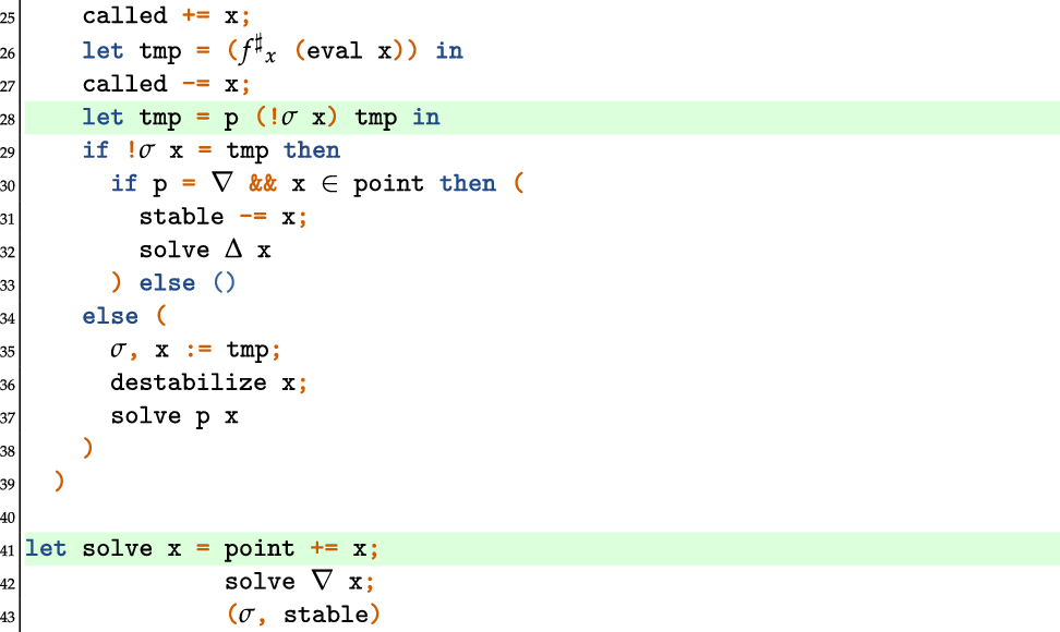
In contrast to algorithm
 $\mathbf{TD}_{\mathbf{term}}$
, the new solver maintains abstract values only for widening and narrowing points as collected in the set
$\mathbf{TD}_{\mathbf{term}}$
, the new solver maintains abstract values only for widening and narrowing points as collected in the set
 $\textit{point}$
. The intuition is that the current values in
$\textit{point}$
. The intuition is that the current values in
 $\sigma$
for all other unknowns can be reconstructed by evaluating their right-hand sides. Thus, we only call
$\sigma$
for all other unknowns can be reconstructed by evaluating their right-hand sides. Thus, we only call
 $\textsf{solve}$
for unknowns in
$\textsf{solve}$
for unknowns in
 $\textit{point}$
, which is why we now always perform widening or narrowing in
$\textit{point}$
, which is why we now always perform widening or narrowing in
 $\textsf{solve}$
.
$\textsf{solve}$
.
We remark that in absence of procedure calls, the set
 $\textit{point}$
may be statically chosen as the set of loop heads – given that each loop is dominated by a single program point. In presence of procedure calls, however, this is no longer easily possible.
$\textit{point}$
may be statically chosen as the set of loop heads – given that each loop is dominated by a single program point. In presence of procedure calls, however, this is no longer easily possible.
Example 11 Consider again the example program from Figure 1, and the corresponding elaborated right-hand sides from Example 5. For the assignment
 $\sigma$
with
$\sigma$
with
 $\sigma{\langle3,a\rangle} = \sigma{\langle4,a\rangle} = \sigma{\langle6,a\rangle} = a$
and
$\sigma{\langle3,a\rangle} = \sigma{\langle4,a\rangle} = \sigma{\langle6,a\rangle} = a$
and
 $\sigma{\langle5,a\rangle} = h^\sharp{}_1\,a$
, the right-hand side of unknown
$\sigma{\langle5,a\rangle} = h^\sharp{}_1\,a$
, the right-hand side of unknown
 ${\langle7,a\rangle}$
accesses, for example, the unknown
${\langle7,a\rangle}$
accesses, for example, the unknown
 ${\langle7,\sigma{\langle5,a\rangle}\rangle} = {\langle7,h^\sharp{}_1\,a\rangle}$
which may put
${\langle7,\sigma{\langle5,a\rangle}\rangle} = {\langle7,h^\sharp{}_1\,a\rangle}$
which may put
 ${\langle7,a\rangle}$
into
${\langle7,a\rangle}$
into
 $\textit{point}$
only if
$\textit{point}$
only if
 $(h^\sharp{}_1)^r a = a$
for some
$(h^\sharp{}_1)^r a = a$
for some
 $r>0$
. The call
$r>0$
. The call
 $\textsf{eval}\,x\,y$
behaves the same as before for unknowns
$\textsf{eval}\,x\,y$
behaves the same as before for unknowns
 $y\in\textit{point}$
. For unknowns
$y\in\textit{point}$
. For unknowns
 $y\not\in\textit{point}$
, the value now must be recovered. For that, y first is marked as
$y\not\in\textit{point}$
, the value now must be recovered. For that, y first is marked as
 $\textit{called}$
. Then, the right-hand side of y is evaluated (still passing x as first argument to eval); finally, y is again removed from
$\textit{called}$
. Then, the right-hand side of y is evaluated (still passing x as first argument to eval); finally, y is again removed from
 $\textit{called}$
. If y is still not in
$\textit{called}$
. If y is still not in
 $\textit{point}$
, the result for y is plainly returned. If, however, the evaluation of
$\textit{point}$
, the result for y is plainly returned. If, however, the evaluation of
 $f^\sharp{}_y$
has inserted y into the set
$f^\sharp{}_y$
has inserted y into the set
 $\textit{point}$
, the function
$\textit{point}$
, the function
 $\textsf{eval}$
proceeds as if y had been contained in
$\textsf{eval}$
proceeds as if y had been contained in
 $\textit{point}$
right from the beginning. This means that
$\textit{point}$
right from the beginning. This means that
 $\textsf{solve}\,\nabla\,y$
is called, x is inserted into the set
$\textsf{solve}\,\nabla\,y$
is called, x is inserted into the set
 $\textit{infl}\,y$
, and subsequently, the value of
$\textit{infl}\,y$
, and subsequently, the value of
 $\sigma$
for y is returned.
$\sigma$
for y is returned.
We remark that on some inputs, the solver
 $\mathbf{TD}_{\mathbf{space}}$
may be rather inefficient, since the same unknown
$\mathbf{TD}_{\mathbf{space}}$
may be rather inefficient, since the same unknown
 $y\not\in\textit{point}$
must be re-evaluated whenever the value of y is queried. At the expense of slightly more space, this deficiency can be remedied by maintaining the values for these unknowns encountered during the re-evaluation of the right-hand side of some unknown
$y\not\in\textit{point}$
must be re-evaluated whenever the value of y is queried. At the expense of slightly more space, this deficiency can be remedied by maintaining the values for these unknowns encountered during the re-evaluation of the right-hand side of some unknown
 $x\in\textit{point}$
in a separate map
$x\in\textit{point}$
in a separate map
 $\tau$
(see the algorithm in Section B of the appendix).
$\tau$
(see the algorithm in Section B of the appendix).
8. Termination and Correctness of TDspace
In the following, we convince ourselves that the solver
 $\mathbf{TD}_{\mathbf{space}}$
has the same termination behavior as the solver
$\mathbf{TD}_{\mathbf{space}}$
has the same termination behavior as the solver
 $\mathbf{TD}_{\mathbf{term}}$
.
$\mathbf{TD}_{\mathbf{term}}$
.
For a finite subset of unknowns
 $Y\subseteq\mathcal{X}^\sharp$
, we construct from
$Y\subseteq\mathcal{X}^\sharp$
, we construct from
 $\mathbb{E}^\sharp$
the residual system
$\mathbb{E}^\sharp$
the residual system
 $\mathbb{E}^\sharp{}_Y$
where the right-hand sides
$\mathbb{E}^\sharp{}_Y$
where the right-hand sides
 $\bar f^\sharp_{Y,y}$
are obtained from the right-hand sides
$\bar f^\sharp_{Y,y}$
are obtained from the right-hand sides
 $f^\sharp_y$
successively exploring the right-hand sides of unknowns not contained in Y. Technically, this means that for
$f^\sharp_y$
successively exploring the right-hand sides of unknowns not contained in Y. Technically, this means that for
 $y\in Y$
and
$y\in Y$
and
 $\sigma:Y\to\mathcal{M}(\mathbb{D})$
,
$\sigma:Y\to\mathcal{M}(\mathbb{D})$
,
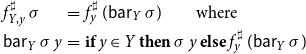 \begin{equation*}\begin{array}{lll}f^\sharp_{Y,y}\,\sigma &=& f^\sharp_y\,(\textsf{bar}_Y\,\sigma)\qquad\text{where} \\\textsf{bar}_Y\,\sigma\,y &=& \textbf{if}\;y\in Y\;\textbf{then}\;\sigma\,y\; \textbf{else}\;f^\sharp_y\,(\textsf{bar}_Y\,\sigma)\end{array}\end{equation*}
Example 12 Consider the monadic right-hand side
 $f^\sharp_{{\langle7,a\rangle}}$
from Example 3 for the program from Figure 1, and
$f^\sharp_{{\langle7,a\rangle}}$
from Example 3 for the program from Figure 1, and
 $Y=\{{\langle7,a\rangle}\mid a\in\mathbb{D}\}$
, we have
$Y=\{{\langle7,a\rangle}\mid a\in\mathbb{D}\}$
, we have
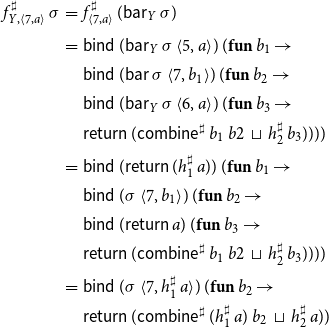 \begin{equation*}\begin{array}{lll}f^\sharp_{Y,{\langle7,a\rangle}}\,\sigma &=& f^\sharp_{{\langle7,a\rangle}}\,(\textsf{bar}_Y\,\sigma) \\[0.5ex] &=& \textsf{bind}\,(\textsf{bar}_Y\,\sigma\,{\langle5,a\rangle})\,(\textbf{fun}\,b_1\to \\ & & \textsf{bind}\,(\textsf{bar}\,\sigma\,{\langle7,b_1\rangle})\,(\textbf{fun}\,b_2\to \\ & & \textsf{bind}\,(\textsf{bar}_Y\,\sigma\,{\langle6,a\rangle})\,(\textbf{fun}\,b_3\to \\ & & \textsf{return}\,(\textsf{combine}^\sharp\,b_1\,b2\;\sqcup\;h^\sharp_2\,b_3)))) \\[0.5ex] &=& \textsf{bind}\,(\textsf{return}\,(h^\sharp_1\,a))\,(\textbf{fun}\,b_1\to \\ & & \textsf{bind}\,(\sigma\,{\langle7,b_1\rangle})\,(\textbf{fun}\,b_2\to \\ & & \textsf{bind}\,(\textsf{return}\,a)\,(\textbf{fun}\,b_3\to \\ & & \textsf{return}\,(\textsf{combine}^\sharp\,b_1\,b2\;\sqcup\;h^\sharp_2\,b_3)))) \\[0.5ex] &=& \textsf{bind}\,(\sigma\,{\langle7,h^\sharp_1\,a\rangle})\,(\textbf{fun}\,b_2\to \\ & & \textsf{return}\,(\textsf{combine}^\sharp\,(h^\sharp_1\,a)\,b_2\;\sqcup\;h^\sharp_2\,a))\end{array}\end{equation*}
In general, let
 $F^\sharp{}_{Y,y}$
be the elaboration of
$F^\sharp{}_{Y,y}$
be the elaboration of
 $f^\sharp_{Y,y}$
. For some
$f^\sharp_{Y,y}$
. For some
 $y\in Y$
and some
$y\in Y$
and some
 $\sigma$
, the evaluation of the right-hand side
$\sigma$
, the evaluation of the right-hand side
 $f^\sharp_{Y,y}$
may not terminate – in which case,
$f^\sharp_{Y,y}$
may not terminate – in which case,
 $F^\sharp{}_{Y,y}\,\sigma$
is undefined. For
$F^\sharp{}_{Y,y}\,\sigma$
is undefined. For
 $\subseteq Y$
, let us call
$\subseteq Y$
, let us call
 $\sigma$
 $(Y,\textit{dom})$
-consistent if
$(Y,\textit{dom})$
-consistent if
 $F^\sharp{}_{Y,y}\,\sigma$
is defined for all
$F^\sharp{}_{Y,y}\,\sigma$
is defined for all
 $y\in \textit{dom}$
. In that case, there is a set
$y\in \textit{dom}$
. In that case, there is a set
 $\bar Y=Y\cup\{y_1,\ldots,y_h\}\subseteq\mathcal{X}$
together with a map
$\bar Y=Y\cup\{y_1,\ldots,y_h\}\subseteq\mathcal{X}$
together with a map
 $\bar\sigma : \bar Y\to\mathbb{D}$
such that
$\bar\sigma : \bar Y\to\mathbb{D}$
such that
 $\bar\sigma|_Y=\sigma$
, and
$\bar\sigma|_Y=\sigma$
, and
-
1.
$(F^\sharp{}_{y_j}\,\bar\sigma)_1=\bar\sigma\,y_j$
and
$(F^\sharp{}_{y_j}\,\bar\sigma)_2\subseteq\bar Y\cup\{y_1,\ldots,y_{j-1}\}$
for all
$j=1,\ldots,h$
; and -
2.
$(F^\sharp{}_{y}\,\bar\sigma)_2\subseteq\bar Y$
for all
$y\in \textit{dom}$
.


The values of the unknowns in
 $\bar Y$
thus are sufficient to evaluate all right-hand sides of unknowns in
$\bar Y$
thus are sufficient to evaluate all right-hand sides of unknowns in
 $\textit{dom}\cup(\bar Y\backslash Y)$
, while the values of
$\textit{dom}\cup(\bar Y\backslash Y)$
, while the values of
 $\bar Y\setminus Y$
can be recovered from the values of the unknowns in Y.
$\bar Y\setminus Y$
can be recovered from the values of the unknowns in Y.
Example 13. Continuing with Example 12, we have that the elaborated right-hand side
 $F^\sharp{}_{Y,{\langle7,a\rangle}}$
is given by:
$F^\sharp{}_{Y,{\langle7,a\rangle}}$
is given by:
 \begin{equation*}\begin{array}{lll}F^\sharp{}_{Y,{\langle7,a\rangle}}\,\sigma &=& \begin{array}[t]{@{}l} (\textsf{combine}^\sharp\,(h^\sharp_1\,a)\,(\sigma\,{\langle7,h^\sharp_1\,a\rangle})\,\sqcup\,h^\sharp{}_2\,a, \{{\langle7,h^\sharp_1\,a\rangle}\}) \end{array}\end{array}\end{equation*}
where the required auxiliary unknowns y are given by
 \begin{equation*}\begin{array}{l}{\langle3,a\rangle},{\langle4,a\rangle},{\langle5,a\rangle},{\langle6,a\rangle}\end{array}\end{equation*}
Subsequently, we adapt the notion of consistency from Section 5 to the case where values from
 $\mathbb{D}$
are only recorded for unknowns in
$\mathbb{D}$
are only recorded for unknowns in
 $\textit{point}$
. Moreover, we maintain that
$\textit{point}$
. Moreover, we maintain that
 $\textit{stable}$
as well as all sets
$\textit{stable}$
as well as all sets
 $\textit{infl}\,y$
are all subsets of
$\textit{infl}\,y$
are all subsets of
 $\textit{point}$
. We now call a solver state
$\textit{point}$
. We now call a solver state
 $s=(\sigma,\textit{infl},\textit{stable},\textit{called},\textit{point})$
consistent if for
$s=(\sigma,\textit{infl},\textit{stable},\textit{called},\textit{point})$
consistent if for
 $Y=(\textit{stable}\cup\textit{called})\cap\textit{point}$
and
$Y=(\textit{stable}\cup\textit{called})\cap\textit{point}$
and
 $\textit{dom}=\textit{stable}\backslash\textit{called}$
,
$\textit{dom}=\textit{stable}\backslash\textit{called}$
,
-
1.
$\sigma$
is
$(Y,\textit{dom})$
-consistent; -
2. for all
$x\in \textit{dom}$
and all
$y \in (F^\sharp{}_{Y,x}\,\sigma)_2$
,
$y\in Y$
and
$x\in\textit{infl}\,y$
holds; -
3. for each
$x\not\in Y$
,
$\textit{infl}\,x=\unicode{x00D8}$
.


With this new notion, the invariants for the calls
 $\textsf{solve}\,p\,x$
, and
$\textsf{solve}\,p\,x$
, and
 $\textsf{destabilize}\,x$
from Section 5, now stay literally the same – with the extra assumption that x should necessarily be contained in
$\textsf{destabilize}\,x$
from Section 5, now stay literally the same – with the extra assumption that x should necessarily be contained in
 $\textit{point}$
. For
$\textit{point}$
. For
 $\textsf{eval}\,x\,y$
, the new invariant must distinguish whether y is contained in
$\textsf{eval}\,x\,y$
, the new invariant must distinguish whether y is contained in
 $\textit{point}$
or not. Assuming that the solver state
$\textit{point}$
or not. Assuming that the solver state
 $s=(\sigma,\textit{infl},\textit{stable},\textit{called},\textit{point})$
before the call is consistent where
$s=(\sigma,\textit{infl},\textit{stable},\textit{called},\textit{point})$
before the call is consistent where
 $x\in\textit{stable}\cap\textit{called}\cap\textit{point}$
, the solver state
$x\in\textit{stable}\cap\textit{called}\cap\textit{point}$
, the solver state
 $s'=(\sigma',\textit{infl}',\textit{stable}',\textit{called}',\textit{point}')$
after the call should now satisfy:
$s'=(\sigma',\textit{infl}',\textit{stable}',\textit{called}',\textit{point}')$
after the call should now satisfy:
-
1. s’ is again consistent;
-
2.
$\textit{called}=\textit{called}'$
, and -
3.
$\textit{stable}\subseteq\textit{stable}'$
where for all
$y'\in(\textit{stable}\cup\textit{called})\cap\textit{point}$
,
$\sigma'\,y'=\sigma\,y'$
and
$\textit{infl}\,y'\subseteq\textit{infl}'\,y'$
; -
4.
$\textit{point}\subseteq\textit{point}'$
where
$y\in\textit{point}'$
whenever
$y\in\textit{called}$
; -
5. If
$y\in(\textit{stable}\cup\textit{called})\cap\textit{point}$
, then -
−
$\sigma = \sigma'$
,
$\textit{stable}=\textit{stable}'$
and
$\textit{point} = \textit{point}'$
; -
−
$\textit{infl}'\,y'=\textit{infl}'\,y'$
for all
$y'\neq y$
, and -
−
$\textit{infl}'\,y= \textit{infl}\,y\cup\{x\}$
. -
6. In all cases when
$y\in\textit{point}'$
, then
$y\in\textit{stable}'$
and
$x\in\textit{infl}'\,y$
and the value
$\sigma'\,y$
is returned; -
7. If
$y\not\in\textit{point}'$
, then
$F^\sharp{}_{Y',y}\,\sigma'$
is defined and produces the return value where
${Y'}=(\textit{stable}'\cup\textit{called}')\cap\textit{point}'$
.


In particular, x is still contained in
 $\textit{stable}'\cap\textit{called}'$
. What we additionally need is an extra argument why evaluation of the right-hand sides of unknowns
$\textit{stable}'\cap\textit{called}'$
. What we additionally need is an extra argument why evaluation of the right-hand sides of unknowns
 $y\not\in\textit{point}$
will necessarily terminate. For that, we observe that, according to our assumption, evaluation of each right-hand side
$y\not\in\textit{point}$
will necessarily terminate. For that, we observe that, according to our assumption, evaluation of each right-hand side
 $f^\sharp{}_y$
will access only finitely many unknowns from
$f^\sharp{}_y$
will access only finitely many unknowns from
 $\mathcal{X}$
. Also, we note that before evaluation of
$\mathcal{X}$
. Also, we note that before evaluation of
 $f^\sharp{}_y$
, the set
$f^\sharp{}_y$
, the set
 $\textit{called}$
additionally receives the unknown y. An unknown z accessed during the evaluation of the right-hand side
$\textit{called}$
additionally receives the unknown y. An unknown z accessed during the evaluation of the right-hand side
 $f^\sharp{}_y$
can only be found not in
$f^\sharp{}_y$
can only be found not in
 $\textit{point}$
, if
$\textit{point}$
, if
 $z\not\in\textit{called}\cup\{y\}$
, that is, each unknown into which recursive evaluation descends must be different from all unknowns added to the set
$z\not\in\textit{called}\cup\{y\}$
, that is, each unknown into which recursive evaluation descends must be different from all unknowns added to the set
 $\textit{called}$
so far.
$\textit{called}$
so far.
Assuming that altogether only finitely many unknowns are encountered during solving, recursive evaluation will eventually terminate having called finitely many times
 $\textsf{solve}$
for unknowns in
$\textsf{solve}$
for unknowns in
 $\textit{point}$
. Therefore, we can adapt the proof of Theorem 1 to obtain:
$\textit{point}$
. Therefore, we can adapt the proof of Theorem 1 to obtain:
Theorem 3. Let
 $\mathbb{E}^\sharp$
denote an arbitrary system of abstract equations, and
$\mathbb{E}^\sharp$
denote an arbitrary system of abstract equations, and
 $x_0\in\mathcal{X}^\sharp$
the unknown of interest. Assume that initially the sets
$x_0\in\mathcal{X}^\sharp$
the unknown of interest. Assume that initially the sets
 $\textit{called}$
and
$\textit{called}$
and
 $\textit{stable}$
are empty, and likewise,
$\textit{stable}$
are empty, and likewise,
 $\textit{infl}$
maps each unknown to the empty set. Assume further that
$\textit{infl}$
maps each unknown to the empty set. Assume further that
 $x\in\textit{point}$
. Then, the call
$x\in\textit{point}$
. Then, the call
 $\textsf{solve}\,x_0$
of solver
$\textsf{solve}\,x_0$
of solver
 $\mathbf{TD}_{\mathbf{space}}$
will always terminate, as long as only finitely many unknowns are encountered.
$\mathbf{TD}_{\mathbf{space}}$
will always terminate, as long as only finitely many unknowns are encountered.
The notion of saturation of solver states literally stays the same. Let
 $s=(\sigma,\textit{infl},\textit{stable},\textit{called},\textit{point})$
denote a consistent solver state. Let
$s=(\sigma,\textit{infl},\textit{stable},\textit{called},\textit{point})$
denote a consistent solver state. Let
 $\tau : \textit{called}\to\mathbb{D}$
denote the restriction of
$\tau : \textit{called}\to\mathbb{D}$
denote the restriction of
 $\sigma$
to the set
$\sigma$
to the set
 $\textit{called}$
. We call s saturated if for all
$\textit{called}$
. We call s saturated if for all
 $x\in \textit{stable}\setminus\textit{called}$
,
$x\in \textit{stable}\setminus\textit{called}$
,
 $\underline\sigma\,x \sqsubseteq \sigma\,x$
where
$\underline\sigma\,x \sqsubseteq \sigma\,x$
where
 $(\underline\sigma,X^\sharp\setminus\textit{called})$
is the least total solution of the lower monotonization of
$(\underline\sigma,X^\sharp\setminus\textit{called})$
is the least total solution of the lower monotonization of
 $\mathbb{E}^\sharp{}_\tau$
. For the space-efficient solver
$\mathbb{E}^\sharp{}_\tau$
. For the space-efficient solver
 $\mathbf{TD}_{\mathbf{space}}$
, Theorem 2 must be re-phrased as follows:
$\mathbf{TD}_{\mathbf{space}}$
, Theorem 2 must be re-phrased as follows:
Theorem 4. Let
 $x\in\textit{point}$
, and consider a call
$x\in\textit{point}$
, and consider a call
 $\textsf{solve}\,\nabla\,x$
encountered by the solver
$\textsf{solve}\,\nabla\,x$
encountered by the solver
 $\mathbf{TD}_{\mathbf{space}}$
during the evaluation of the initial call. Then it always starts in a saturated solver state, and upon termination, it results in a solver state
$\mathbf{TD}_{\mathbf{space}}$
during the evaluation of the initial call. Then it always starts in a saturated solver state, and upon termination, it results in a solver state
 $s' = (\sigma' ,\textit{infl}',\textit{stable}',\textit{called}',\textit{point}')$
which is again saturated so that
$s' = (\sigma' ,\textit{infl}',\textit{stable}',\textit{called}',\textit{point}')$
which is again saturated so that
 $x\in\textit{stable}'$
. The proof is along the same lines as the proof for Theorem 2 – only that now the assignment
$x\in\textit{stable}'$
. The proof is along the same lines as the proof for Theorem 2 – only that now the assignment
 $\sigma$
must be replaced with Y-consistent mappings
$\sigma$
must be replaced with Y-consistent mappings
 $\bar\sigma{}_Y$
for suitable Y with
$\bar\sigma{}_Y$
for suitable Y with
 $\textit{stable}\setminus\textit{called}\subseteq Y\subseteq\textit{stable}'\setminus\textit{called}$
.
$\textit{stable}\setminus\textit{called}\subseteq Y\subseteq\textit{stable}'\setminus\textit{called}$
.
Proof. Let
 $\mathcal{X}'$
denote the set of all unknowns in
$\mathcal{X}'$
denote the set of all unknowns in
 $\textit{stable}'\setminus\textit{called}'$
. In particular,
$\textit{stable}'\setminus\textit{called}'$
. In particular,
 $x\in\mathcal{X}'$
. We proceed by induction on the set of unknowns not contained in the set
$x\in\mathcal{X}'$
. We proceed by induction on the set of unknowns not contained in the set
 $\mathcal{X}{}_0$
of called unknowns. Again, we concentrate on the last tail-recursive call
$\mathcal{X}{}_0$
of called unknowns. Again, we concentrate on the last tail-recursive call
 $\textsf{solve}\,\nabla\,x$
before the call to
$\textsf{solve}\,\nabla\,x$
before the call to
 $\textsf{solve}\,\Delta\,x$
. Let d denote the value of x before the evaluation of the right-hand side, and d’ the value returned by evaluating the right-hand side. Let
$\textsf{solve}\,\Delta\,x$
. Let d denote the value of x before the evaluation of the right-hand side, and d’ the value returned by evaluating the right-hand side. Let
 $\mathcal{X}'$
denote the set of unknowns accessed during the call. Since subsequently
$\mathcal{X}'$
denote the set of unknowns accessed during the call. Since subsequently
 $\textsf{solve}\,\Delta\,x$
is called, after that call x is contained in
$\textsf{solve}\,\Delta\,x$
is called, after that call x is contained in
 $\textit{stable}$
. Therefore, one of the following two situations is encountered after the evaluation of the right-hand side:
$\textit{stable}$
. Therefore, one of the following two situations is encountered after the evaluation of the right-hand side:
-
1.
$d'\sqsubseteq d$
, that is, the value d’ is subsumed by the current value of x; or -
2. subsequent destabilization will not destabilize x.

In the second case, the unknowns that directly or indirectly influence x do cannot depend on x (w.r.t. the current sets
 $\textit{infl}$
). Thus, a similar argument as for unknowns not in
$\textit{infl}$
). Thus, a similar argument as for unknowns not in
 $\textit{point}$
in the proof of Theorem 2 applies. Accordingly, it remains to consider the first case. Let Y denote the set
$\textit{point}$
in the proof of Theorem 2 applies. Accordingly, it remains to consider the first case. Let Y denote the set
 $\textit{stable}\cup\textit{called}$
in the current solver state, and
$\textit{stable}\cup\textit{called}$
in the current solver state, and
 $\tau$
the restriction of
$\tau$
the restriction of
 $\sigma$
to
$\sigma$
to
 $\textit{called}\cap\textit{point}$
, extended with
$\textit{called}\cap\textit{point}$
, extended with
 $\{y\mapsto\bot\mid y\in\textit{called}\setminus\textit{point}\}$
. Consider the lower monotonizations of the abstract systems
$\{y\mapsto\bot\mid y\in\textit{called}\setminus\textit{point}\}$
. Consider the lower monotonizations of the abstract systems
 $\mathbb{E}^\sharp{}_\tau$
and
$\mathbb{E}^\sharp{}_\tau$
and
 $\mathbb{E}^\sharp{}_{\tau\oplus\{x\mapsto d\}}$
with least solutions
$\mathbb{E}^\sharp{}_{\tau\oplus\{x\mapsto d\}}$
with least solutions
 $\underline\sigma$
and
$\underline\sigma$
and
 $\underline\sigma'$
, respectively. Let
$\underline\sigma'$
, respectively. Let
 $\sigma{}_0$
denote the assignment to the unknowns in
$\sigma{}_0$
denote the assignment to the unknowns in
 $\mathcal{X}^\sharp\setminus(\mathcal{X}{}_0\cup\{x\})$
before the call
$\mathcal{X}^\sharp\setminus(\mathcal{X}{}_0\cup\{x\})$
before the call
 $\textsf{solve}\,\Delta\,x$
. By inductive hypothesis applied to the unknowns in
$\textsf{solve}\,\Delta\,x$
. By inductive hypothesis applied to the unknowns in
 $\mathcal{X}'\setminus\{x\}$
and
$\mathcal{X}'\setminus\{x\}$
and
 $\tau\oplus\{x\mapsto d\}$
, we find that
$\tau\oplus\{x\mapsto d\}$
, we find that
 $\underline\sigma'\,y\sqsubseteq\sigma{}_0\,y$
for all unknowns
$\underline\sigma'\,y\sqsubseteq\sigma{}_0\,y$
for all unknowns
 $y\in\mathcal{X}'\setminus\{x\}$
where
$y\in\mathcal{X}'\setminus\{x\}$
where
 $\underline\sigma'\oplus\{x\mapsto d\}$
is a post-solution of the lower monotonization of
$\underline\sigma'\oplus\{x\mapsto d\}$
is a post-solution of the lower monotonization of
 $\mathbb{E}^\sharp{}_\tau$
. Therefore,
$\mathbb{E}^\sharp{}_\tau$
. Therefore,
 $\underline\sigma\,y\sqsubseteq\underline\sigma'\oplus\{x\mapsto d\} \sqsubseteq(\sigma{}_0\oplus\{x\mapsto d\})\,y$
for all
$\underline\sigma\,y\sqsubseteq\underline\sigma'\oplus\{x\mapsto d\} \sqsubseteq(\sigma{}_0\oplus\{x\mapsto d\})\,y$
for all
 $y\in\mathcal{X}'$
holds, and the claim follows. Now consider the narrowing iteration performed for x in the subsequent call
$y\in\mathcal{X}'$
holds, and the claim follows. Now consider the narrowing iteration performed for x in the subsequent call
 $\textsf{solve}\,\Delta\,x$
. Let
$\textsf{solve}\,\Delta\,x$
. Let
 $d_0$
denote the value after the last call to
$d_0$
denote the value after the last call to
 $\textsf{solve}\,\nabla\,x$
, and
$\textsf{solve}\,\nabla\,x$
, and
 $d_1,\ldots, d_k$
denote the values returned by evaluating the right-hand side of x during this iteration, and define
$d_1,\ldots, d_k$
denote the values returned by evaluating the right-hand side of x during this iteration, and define
 $d'_0 = d_0$
and for
$d'_0 = d_0$
and for
 $i>0$
,
$i>0$
,
 $d'_i = d'_{i-1}\Delta d_i$
. Let
$d'_i = d'_{i-1}\Delta d_i$
. Let
 $\sigma{}_i$
denote the assignment attained after the ith narrowing step restricted to the unknowns
$\sigma{}_i$
denote the assignment attained after the ith narrowing step restricted to the unknowns
 $\mathcal{X}^\sharp\setminus(\mathcal{X}{}_0\cup\{x\})$
. For
$\mathcal{X}^\sharp\setminus(\mathcal{X}{}_0\cup\{x\})$
. For
 $i>0$
, let
$i>0$
, let
 $\underline\sigma{}_i$
denote the least solution of the lower monotonization of
$\underline\sigma{}_i$
denote the least solution of the lower monotonization of
 $\mathbb{E}^\sharp{}_{\tau\oplus\{x\mapsto d_{i-1}\}}$
. By inductive hypothesis,
$\mathbb{E}^\sharp{}_{\tau\oplus\{x\mapsto d_{i-1}\}}$
. By inductive hypothesis,
 $\underline\sigma{}_i\,y\sqsubseteq\sigma{}_i$
for all
$\underline\sigma{}_i\,y\sqsubseteq\sigma{}_i$
for all
 $y\neq x$
which are stable after the ith iteration. By induction on i, we prove that
$y\neq x$
which are stable after the ith iteration. By induction on i, we prove that
 $\underline\sigma\,x\sqsubseteq d_i$
and thus also
$\underline\sigma\,x\sqsubseteq d_i$
and thus also
 $\underline\sigma\,x\sqsubseteq d'_i$
, and
$\underline\sigma\,x\sqsubseteq d'_i$
, and
 $\underline\sigma\,y\sqsubseteq\sigma{}_i\,y$
for every
$\underline\sigma\,y\sqsubseteq\sigma{}_i\,y$
for every
 $y\in\mathcal{X}^\sharp\setminus(\mathcal{X}{}_0\cup\{x\})$
which is stable after the ith narrowing iteration. This assertion holds for
$y\in\mathcal{X}^\sharp\setminus(\mathcal{X}{}_0\cup\{x\})$
which is stable after the ith narrowing iteration. This assertion holds for
 $i=0$
. For
$i=0$
. For
 $i>0$
, the assertion on the
$i>0$
, the assertion on the
 $y\neq x$
follows by inductive hypothesis for a larger set of called unknowns. And for x, we have
$y\neq x$
follows by inductive hypothesis for a larger set of called unknowns. And for x, we have
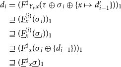 \begin{equation*}\begin{array}{lcl}d_i &=& (F^\sharp{}_{Y_i,x}(\tau\oplus\sigma{}_i\oplus\{x\mapsto d'_{i-1}\}))_1 \\ &\sqsupseteq&(\underline F^{(i)}_{x}(\sigma{}_i))_1 \\ &\sqsupseteq&(\underline F^{(i)}_{x}(\underline\sigma{}_i))_1 \\ &\sqsupseteq&(\underline F^\sharp{}_{x}(\underline\sigma{}_i\oplus\{d_{i-1}\}))_1 \\ &\sqsupseteq&(\underline F^\sharp{}_{x}\underline\sigma)_1\end{array}\end{equation*}
Here,
 $F^\sharp{}_{Y_i,x}$
is the elaborated right-hand side for
$F^\sharp{}_{Y_i,x}$
is the elaborated right-hand side for
 $f^\sharp_{x}\circ\textsf{bar}_{Y_i}$
where
$f^\sharp_{x}\circ\textsf{bar}_{Y_i}$
where
 $Y_i$
equals the union of the set
$Y_i$
equals the union of the set
 $\textit{point}\cup\textit{called}$
after the ith iteration of
$\textit{point}\cup\textit{called}$
after the ith iteration of
 $\textsf{solve}\,\Delta\,x$
. Moreover,
$\textsf{solve}\,\Delta\,x$
. Moreover,
 $\underline F^\sharp{}_{x}$
and
$\underline F^\sharp{}_{x}$
and
 $\underline F^{(i)}_{x}$
are the right-hand sides of the lower monotonizations of
$\underline F^{(i)}_{x}$
are the right-hand sides of the lower monotonizations of
 $\mathbb{E}^\sharp{}_\tau$
and
$\mathbb{E}^\sharp{}_\tau$
and
 $\mathbb{E}^\sharp{}_{\tau\oplus\{x\mapsto d_{i-1}\}}$
for x, respectively. This completes the proof of the theorem.
$\mathbb{E}^\sharp{}_{\tau\oplus\{x\mapsto d_{i-1}\}}$
for x, respectively. This completes the proof of the theorem.
9. Side-Effecting Systems of Equations
Concurrency libraries such as Posix threads (Walli Reference Walli1995) or OSEK (Lemieux Reference Lemieux2001) support communication between threads by means of shared program variables and data structures, while primitives such as mutexes or resources are provided to synchronize their executions.
Example 14. Consider the program
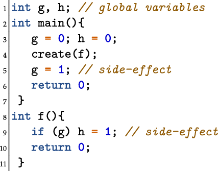
with global variables g,h, where the call create(f) is meant to spawn a new thread which executes the parameterless function f. The function main thus first initializes the globals g,h. Then, a thread is spawned executing the function f. Finally, g is set to 1, followed by returning with 0. The function f, when executed, checks the global variable g. If it is different from 0, 1 is assigned to h. Finally, 0 is returned. Accordingly, the two threads communicate via the shared program variable g.
One natural way to de-couple the analysis of multi-threaded code is to interprocedurally analyze only the thread-local states, while a flow-insensitive global invariant is accumulated for shared data (Seidl and Vogler Reference Seidl, Vogler, D’Souza and Narayan Kumar2017; Vojdani and Vene Reference Vojdani and Vene2009). This idea is realized in the analyzer Goblint (Vojdani et al. Reference Vojdani, Apinis, RÕtov, Seidl, Vene and Vogler2016). To a certain extent, this approach can be accommodated also to analyses taking mutexes into account such as Mine (2012, 2014). One way of conveniently combining flow-insensitive analysis of shared data with context-sensitive analysis of local state is by extending systems of equations with side effects (Apinis et al. Reference Apinis, Seidl, Vojdani and Igarashi2012). Side effects during solving should be seen in analogy to the meta-predicate assert in Prolog clauses: while computing a contribution to the predicate of the head, a contribution to some other predicate is triggered. A right-hand side function
 $f^\sharp{}_x$
in monadic form now has type:
$f^\sharp{}_x$
in monadic form now has type:
 \begin{equation*}(\mathcal{X}^\sharp\to\mathcal{M}(\mathbb{D}))\to(\mathcal{X}\to\mathbb{D}\to\mathcal{M}(\bullet))\to\mathcal{M}(\mathbb{D})\end{equation*}
for any monad
 $\mathcal{M}$
. The
$\mathcal{M}$
. The
 $\bullet$
here represents the one-element complete lattice
$\bullet$
here represents the one-element complete lattice
 $\bullet=\{()\}$
. The second argument function is meant to be called for triggering side effects. These events are observed by the solver, but otherwise do not affect the computed value. Accordingly, the return values of the second argument function should be in
$\bullet=\{()\}$
. The second argument function is meant to be called for triggering side effects. These events are observed by the solver, but otherwise do not affect the computed value. Accordingly, the return values of the second argument function should be in
 $\mathcal{M}(\bullet)$
.
$\mathcal{M}(\bullet)$
.
Example 15. Consider the program from Example 14. Let us assume that we use intervals as values for each of these unknowns. Since the functions have no local variables, but a return value each, let us represent the local state of a function by a single interval as well which may initially be thought of having value
 $\top = [-\infty,\infty]$
. The part of the system of abstract equations for calling contexts
$\top = [-\infty,\infty]$
. The part of the system of abstract equations for calling contexts
 $\top$
is given by the right-hand sides (in monadic form) of the unknowns g,h as well as
$\top$
is given by the right-hand sides (in monadic form) of the unknowns g,h as well as
 ${\textsf{main}}$
, and f corresponding to the end points of the respective functions:
${\textsf{main}}$
, and f corresponding to the end points of the respective functions:
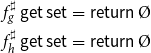 \begin{equation*}\begin{array}{lll} f^\sharp_g\,\textsf{get}\,\textsf{set} &=& \textsf{return}\,\unicode{x00D8} \\ f^\sharp_h\,\textsf{get}\,\textsf{set} &=& \textsf{return}\,\unicode{x00D8} \\\end{array}\end{equation*}
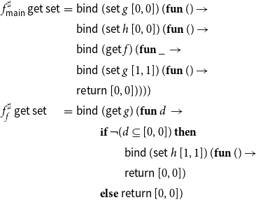 \begin{equation*}\begin{array}{lll} f^\sharp_{{\textsf{main}}}\,\textsf{get}\,\textsf{set} &=& \textsf{bind}\,(\textsf{set}\,g\,[0,0])\,(\textbf{fun}\,()\to\\ & & \textsf{bind}\,(\textsf{set}\,h\,[0,0])\,(\textbf{fun}\,()\to\\ & & \textsf{bind}\,(\textsf{get}\,f)\,(\textbf{fun}\,\_\,\to\\ & & \textsf{bind}\,(\textsf{set}\,g\,[1,1])\,(\textbf{fun}\,()\to\\ & & \textsf{return}\,[0,0])))) \\ f^\sharp_f\,\textsf{get}\,\textsf{set} &=& \textsf{bind}\,(\textsf{get}\,g)\,(\textbf{fun}\,d\,\to \\ & & \qquad\begin{array}[t]{@{}l} \textbf{if}\;\neg(d\subseteq[0,0])\;\textbf{then}\; \\ \qquad\textsf{bind}\,(\textsf{set}\,h\,[1,1])\,(\textbf{fun}\,()\to\\ \qquad\textsf{return}\,[0,0]) \\ \textbf{else}\;\textsf{return}\,[0,0]) \end{array}\end{array}\end{equation*}
The unknowns g and h corresponding to the global variables of the program thus have trivial right-hand sides. Both unknowns are meant to receive their values solely via side effects.
Due to parametricity in the monad, each right-hand side function of a side-effecting abstract system of equations again can be represented by a generalized execution tree
 $t_x$
such that
$t_x$
such that
 $f^\sharp{}_x={t_x}$
. Generalized execution trees now make not only explicit which unknowns are accessed, but also which side effects should be triggered during evaluation. Therefore, they additionally may contain a constructor
$f^\sharp{}_x={t_x}$
. Generalized execution trees now make not only explicit which unknowns are accessed, but also which side effects should be triggered during evaluation. Therefore, they additionally may contain a constructor
 \begin{equation*}\textsf{S}\,(\mathcal{X}^\sharp,\mathbb{D},\mathcal T)\end{equation*}
The intention is that evaluation of
 $\textsf{S}\,(x,d,t)$
first adds
$\textsf{S}\,(x,d,t)$
first adds
 $d\in\mathbb{D}$
to the value of x and then continues with the evaluation of t. Accordingly, the semantics of such a generalized tree t is the function
$d\in\mathbb{D}$
to the value of x and then continues with the evaluation of t. Accordingly, the semantics of such a generalized tree t is the function
 ${t}:(\mathcal{X}^\sharp\to\mathcal{M}(\mathbb{D}))\to (\mathcal{X}^\sharp\to\mathbb{D}\to\mathcal{M}(\bullet))\to \mathcal{M}(\mathbb{D})$
which for functions
${t}:(\mathcal{X}^\sharp\to\mathcal{M}(\mathbb{D}))\to (\mathcal{X}^\sharp\to\mathbb{D}\to\mathcal{M}(\bullet))\to \mathcal{M}(\mathbb{D})$
which for functions
 $\textsf{get}:\mathcal{X}\to\mathcal{M}(\mathbb{D})$
and
$\textsf{get}:\mathcal{X}\to\mathcal{M}(\mathbb{D})$
and
 $\textsf{set}:\mathcal{X}\to\mathbb{D}\to\mathcal{M}(\bullet)$
is defined by
$\textsf{set}:\mathcal{X}\to\mathbb{D}\to\mathcal{M}(\bullet)$
is defined by
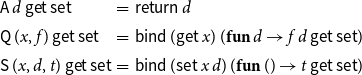 \begin{equation*}\begin{array}{lll} {\textsf{A}\,d}\,\textsf{get}\,\textsf{set} &=& \textsf{return}\,d \\ {\textsf{Q}\,(x,f)}\,\textsf{get}\,\textsf{set} &=& \textsf{bind}\,(\textsf{get}\,x)\, (\textbf{fun}\,d\to {f\,d}\,\textsf{get}\,\textsf{set}) \\ {\textsf{S}\,(x,d,t)}\,\textsf{get}\,\textsf{set} &=& \textsf{bind}\,(\textsf{set}\,x\,d)\,(\textbf{fun}\,()\to{t}\,\textsf{get}\,\textsf{set})\end{array}\end{equation*}
In case of a state transformer monad with set of states S, this amounts to
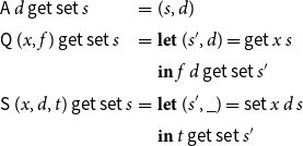 \begin{equation*}\begin{array}{lll} {\textsf{A}\,d}\,\textsf{get}\,\textsf{set}\,s &=& (s,d) \\ {\textsf{Q}\,(x,f)}\,\textsf{get}\,\textsf{set}\,s &=& \textbf{let}\;(s',d) = \textsf{get}\,x\,s \\ & & \textbf{in}\;{f\,d}\,\textsf{get}\,\textsf{set}\,s' \\ {\textsf{S}\,(x,d,t)}\,\textsf{get}\,\textsf{set}\,s &=& \textbf{let}\;(s',\_) = \textsf{set}\,x\,d\,s \\ & & \textbf{in}\;{t}\,\textsf{get}\,\textsf{set}\,s' \\\end{array}\end{equation*}
Consider the set of extended states
 $S = (\mathcal{X}^\sharp\to\mathbb{D})\times \mathcal{P} ({\mathcal{X}^\sharp})\times(\mathcal{X}^\sharp\to\mathbb{D})$
where the third component accumulates side effects. Consider the functions
$S = (\mathcal{X}^\sharp\to\mathbb{D})\times \mathcal{P} ({\mathcal{X}^\sharp})\times(\mathcal{X}^\sharp\to\mathbb{D})$
where the third component accumulates side effects. Consider the functions
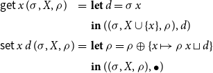 \begin{equation*}\begin{array}{lll} \textsf{get}\,x\,(\sigma,X,\rho) &=& \textbf{let}\;d = \sigma\,x \\ & & \textbf{in}\;((\sigma,X\cup\{x\},\rho),d) \\ \textsf{set}\,x\,d\,(\sigma,X,\rho) &=& \textbf{let}\;\rho = \rho\oplus\{x\mapsto \rho\,x\sqcup d\} \\ & & \textbf{in}\;((\sigma,X,\rho),\bullet) \\\end{array}\end{equation*}
Then, the elaborated right-hand side function
 $F^\sharp{}_x$
has type
$F^\sharp{}_x$
has type
 \begin{equation*}F^\sharp{}_x: (\mathcal{X}^\sharp\to\mathbb{D})\to(\mathbb{D}\times \mathcal{P} ({\mathcal{X}^\sharp})\times(\mathcal{X}^\sharp\to\mathbb{D}))\end{equation*}
where the third component of the result represents the side effects to other unknowns encountered during evaluation of
 $f^\sharp{}_{x}$
. This function is given by:
$f^\sharp{}_{x}$
. This function is given by:
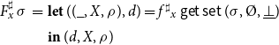 \begin{equation*}\begin{array}{lll}F_x^\sharp\,\sigma &=& \textbf{let}\;((\_,X,\rho),d) = f^\sharp{}_x\,\textsf{get}\,\textsf{set}\,(\sigma,\unicode{x00D8},\underline\bot) \\& & \textbf{in}\; (d,X,\rho)\end{array}\end{equation*}
Example 16. Let us consider the right-hand side functions from Example 15 for the interval analysis of the program in Example 14 at the beginning of this section. These are now are given by
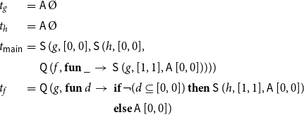 \begin{equation*}\begin{array}{lll} t_g &=& \textsf{A}\,\unicode{x00D8} \\ t_h &=& \textsf{A}\,\unicode{x00D8} \\ t_{{\textsf{main}}} &=& \textsf{S}\,(g,[0,0], \textsf{S}\,(h,[0,0], \\ & & \textsf{Q}\,(f,\textbf{fun}\,\_\,\to \, \textsf{S}\,(g,[1,1],\textsf{A}\,[0,0])))) \\ t_f &=& \textsf{Q}\,(g,\textbf{fun}\,d\,\to\,\begin{array}[t]{@{}l} \textbf{if}\;\neg(d\subseteq[0,0])\;\textbf{then}\; \textsf{S}\,(h,[1,1],\textsf{A}\,[0,0]) \\ \textbf{else}\;\textsf{A}\,[0,0]) \end{array}\end{array}\end{equation*}
The computation tree
 $t_{\textsf{main}}$
for
$t_{\textsf{main}}$
for
 ${\textsf{main}}$
first produces side effects [0,0] onto the unknowns g and h, respectively. Then, it queries the return value of f, but ignores that value. This query enables the local solver to start the evaluation of the unknown f and thus the exploration of the function f. Subsequently, another side effect [1,1] is produced onto the unknown g, before the value [0,0] is returned. The computation tree
${\textsf{main}}$
first produces side effects [0,0] onto the unknowns g and h, respectively. Then, it queries the return value of f, but ignores that value. This query enables the local solver to start the evaluation of the unknown f and thus the exploration of the function f. Subsequently, another side effect [1,1] is produced onto the unknown g, before the value [0,0] is returned. The computation tree
 $t_f$
for f first queries g. Depending on the obtained value, a side effect of [1,1] is produced onto the variable h or omitted. Eventually then the value [0,0] is returned. Elaboration of the right-hand side functions results in the functions
$t_f$
for f first queries g. Depending on the obtained value, a side effect of [1,1] is produced onto the variable h or omitted. Eventually then the value [0,0] is returned. Elaboration of the right-hand side functions results in the functions
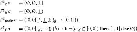 \begin{equation*}\begin{array}{lll} F^\sharp{}_g\,\sigma &=& (\unicode{x00D8},\unicode{x00D8},\underline\bot) \\ F^\sharp{}_h\,\sigma &=& (\unicode{x00D8},\unicode{x00D8},\underline\bot) \\ F^\sharp{}_{{\textsf{main}}}\,\sigma &=& ([0,0],{f},\underline\bot\oplus\{g\mapsto[0,1]\}) \\ F^\sharp{}_f\,\sigma &=& ([0,0],{g}, \underline\bot\oplus\{h\mapsto\textbf{if}\,\neg(\sigma\,g\subseteq[0,0])\, \textbf{then}\,[1,1]\,\textbf{else}\,\unicode{x00D8}\})\end{array}\end{equation*}
Here,
 $\underline\bot$
denotes the assignment mapping each unknown to
$\underline\bot$
denotes the assignment mapping each unknown to
 $\bot$
– which in the example equals
$\bot$
– which in the example equals
 $\unicode{x00D8}$
. As can be seen for
$\unicode{x00D8}$
. As can be seen for
 $\textsf{main}$
, elaborated right-hand side functions may combine multiple side effects to the same unknown (in this case, g) into one and also no longer differentiate when during the evaluation, each side effect is produced.
$\textsf{main}$
, elaborated right-hand side functions may combine multiple side effects to the same unknown (in this case, g) into one and also no longer differentiate when during the evaluation, each side effect is produced.
Side effects also come in handy when only parts of the context are used to discriminate procedure calls (Apinis et al. Reference Apinis, Seidl, Vojdani and Igarashi2012). Assume that we are given a mapping
 $\pi:\mathbb{D}\to A$
for some set A of distinguishing abstract properties of contexts. Consider the abstract effect of a call to a procedure p. Let u,v denote the program points before and after the call, respectively. Then for every abstract context
$\pi:\mathbb{D}\to A$
for some set A of distinguishing abstract properties of contexts. Consider the abstract effect of a call to a procedure p. Let u,v denote the program points before and after the call, respectively. Then for every abstract context
 $a\in A$
, the right-hand side for the unknown
$a\in A$
, the right-hand side for the unknown
 ${\langle v,a\rangle}$
is given by
${\langle v,a\rangle}$
is given by
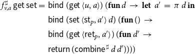 \begin{equation*}f^\sharp_{v,a}\,\textsf{get}\,\textsf{set} = \begin{array}[t]{l} \textsf{bind}\,(\textsf{get}\,{\langle u,a\rangle})\,(\textbf{fun}\,d\,\to\,\textbf{let}\;\; a'\;=\; \pi\,d\;\textbf{in} \\ \textsf{bind}\,(\textsf{set}\,{\langle\textsf{st}_p,a'\rangle}\,d)\,(\textbf{fun}\,()\,\to \\ \textsf{bind}\,(\textsf{get}\,{\langle\textsf{ret}_p,a'\rangle})\,(\textbf{fun}\,d'\,\to \\ \textsf{return}\,(\textsf{combine}^\sharp\,d\,d')))) \end{array}\end{equation*}
or, alternatively, by the computation tree
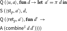 \begin{equation*} \begin{array}[t]{l} \textsf{Q}\,({\langle u,a\rangle},\textbf{fun}\, d \to \textbf{let}\;\; a'= \pi\,d\;\textbf{in} \\ \textsf{S}\,({\langle\textsf{st}_p,a'\rangle}, d, \\ \textsf{Q}\,({\langle\textsf{ret}_p,a'\rangle},\textbf{fun}\,d'\,\to \\ \textsf{A}\,(\textsf{combine}^\sharp\,d\,d')))) \end{array}\end{equation*}
where
 $\textsf{combine}^\sharp : \mathbb{D}\to\mathbb{D}\to\mathbb{D}$
again combines the abstract program state attained at the endpoint
$\textsf{combine}^\sharp : \mathbb{D}\to\mathbb{D}\to\mathbb{D}$
again combines the abstract program state attained at the endpoint
 $\textsf{ret}_p$
of p with the state before the call to the state of the caller after the call.
$\textsf{ret}_p$
of p with the state before the call to the state of the caller after the call.
In this formalization, the side effect to the start point
 $\textsf{st}_p$
of the called procedure p is used to accumulate all values d leading to the same abstract context a’ for which p is analyzed. In order to prove the resulting analysis sound, it is convenient to reformulate also the concrete collecting semantics by introducing side effects. For a concrete program state q, the right-hand side
$\textsf{st}_p$
of the called procedure p is used to accumulate all values d leading to the same abstract context a’ for which p is analyzed. In order to prove the resulting analysis sound, it is convenient to reformulate also the concrete collecting semantics by introducing side effects. For a concrete program state q, the right-hand side
 $\mathbb{E}\,{\langle v,q\rangle}\,\sigma$
for the unknown representing the procedure call in concrete calling context q, is given by
$\mathbb{E}\,{\langle v,q\rangle}\,\sigma$
for the unknown representing the procedure call in concrete calling context q, is given by
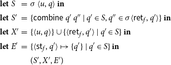 \begin{equation*}\begin{array}{llll}\textbf{let}& S &=& \sigma\,{\langle{u,q}\rangle}\;\textbf{in} \\ \textbf{let}&S'&=& \{\textsf{combine}\,q'\,q''\mid q'\in S, q''\in \sigma{\langle\textsf{ret}_f,q'\rangle}\}\;\textbf{in} \\ \textbf{let}&X'&=& \{{\langle{u,q}\rangle}\}\cup \{{\langle\textsf{ret}_f,q'\rangle}\mid q'\in S\}\;\textbf{in} \\ \textbf{let}&E'&=& \{{\langle\textsf{st}_f,q'\rangle}\mapsto \{q'\} \mid q'\in S\} \;\textbf{in} \\ & & &(S',X',E')\end{array}\end{equation*}
For convenience we here introduce the convention that those unknowns not explicitly listed as arguments in E’ are implicitly all mapped to
 $\bot$
(
$\bot$
(
 $\unicode{x00D8}$
in case of the concrete collecting semantics).
$\unicode{x00D8}$
in case of the concrete collecting semantics).
Interestingly, the description relation
 $\mathrel{\mathcal{R}}$
between unknowns of the concrete and abstract systems can now no longer be specified as is, but must take some over-approximation
$\mathrel{\mathcal{R}}$
between unknowns of the concrete and abstract systems can now no longer be specified as is, but must take some over-approximation
 $\rho$
of all abstract side effects into account. In order to see this, assume for a moment that the set A contains a single element
$\rho$
of all abstract side effects into account. In order to see this, assume for a moment that the set A contains a single element
 $\bullet$
, that is, procedures are analyzed without context. Consider the unknown
$\bullet$
, that is, procedures are analyzed without context. Consider the unknown
 ${\langle\textsf{st}_p,\bullet\rangle}$
for the procedure p. This unknown should describe concrete unknowns
${\langle\textsf{st}_p,\bullet\rangle}$
for the procedure p. This unknown should describe concrete unknowns
 ${\langle\textsf{st}_p,q\rangle}$
– however, not for all program states q. Instead, only those q must be taken into account which actually occur as calling contexts of p in the collecting semantics of the program. A (hopefully not too large) superset of these is given by
${\langle\textsf{st}_p,q\rangle}$
– however, not for all program states q. Instead, only those q must be taken into account which actually occur as calling contexts of p in the collecting semantics of the program. A (hopefully not too large) superset of these is given by
 $\gamma(\rho{\langle\textsf{st}_p,\bullet\rangle})$
if
$\gamma(\rho{\langle\textsf{st}_p,\bullet\rangle})$
if
 $\rho$
is an over-approximation of the side effects encountered during the abstract fixpoint iteration. More generally, we define for interprocedural analysis with a set A of abstract distinguishing contexts,
$\rho$
is an over-approximation of the side effects encountered during the abstract fixpoint iteration. More generally, we define for interprocedural analysis with a set A of abstract distinguishing contexts,
 \begin{equation*}{\langle u',q\rangle} \mathrel{\mathcal{R}_\rho} {\langle u',a\rangle}\quad\text{iff}\quad q\in\gamma(\rho\,{\langle\textsf{st}_p,a\rangle})\end{equation*}
if u’ is a program point of the procedure p and
 $a\in A$
. Subsequently, we therefore assume that we are given a description relation
$a\in A$
. Subsequently, we therefore assume that we are given a description relation
 $\mathrel{\mathcal{R}_\rho} \subseteq \mathcal{X} \times \mathcal{X}^\sharp$
between the concrete and abstract unknowns depending on some over-approximation of the side effects
$\mathrel{\mathcal{R}_\rho} \subseteq \mathcal{X} \times \mathcal{X}^\sharp$
between the concrete and abstract unknowns depending on some over-approximation of the side effects
 $\rho$
. As in Section 3, the description relation
$\rho$
. As in Section 3, the description relation
 $\mathrel{\mathcal{R}_\rho}$
on unknowns is extended to sets of unknowns and assignments to unknowns, right-hand sides and systems of equations. For elaborated right-hand side functions
$\mathrel{\mathcal{R}_\rho}$
on unknowns is extended to sets of unknowns and assignments to unknowns, right-hand sides and systems of equations. For elaborated right-hand side functions
 $F,F^\sharp$
,
$F,F^\sharp$
,
 $F \mathrel{\mathcal{R}_\rho} F^\sharp$
is meant to hold whenever for assignments
$F \mathrel{\mathcal{R}_\rho} F^\sharp$
is meant to hold whenever for assignments
 $\sigma,\sigma^\sharp$
with
$\sigma,\sigma^\sharp$
with
 $\sigma \mathrel{\mathcal{R}_\rho} \sigma^\sharp$
, the following holds:
$\sigma \mathrel{\mathcal{R}_\rho} \sigma^\sharp$
, the following holds:
-
$(F\,\sigma)_1\subseteq\gamma(F^\sharp\,\sigma^\sharp)_1$
;
-
$(F\,\sigma)_2 \mathrel{\mathcal{R}_\rho} (F^\sharp\,\sigma^\sharp)_2$
where
-
$(F\,\sigma)_3 \mathrel{\mathcal{R}_\rho} \rho$
as well as
$(F^\sharp\,\sigma^\sharp)_3\sqsubseteq\rho$
.
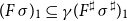
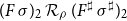


while then for equation systems
 $\mathbb{E},\mathbb{E}^\sharp$
,
$\mathbb{E},\mathbb{E}^\sharp$
,
 $\mathbb{E} \mathrel{\mathcal{R}_\rho} \mathbb{E}^\sharp$
holds if
$\mathbb{E} \mathrel{\mathcal{R}_\rho} \mathbb{E}^\sharp$
holds if
 $F_x \mathrel{\mathcal{R}_\rho} F^\sharp{}_{x^\sharp}$
holds for all unknowns
$F_x \mathrel{\mathcal{R}_\rho} F^\sharp{}_{x^\sharp}$
holds for all unknowns
 $x,x^\sharp$
with
$x,x^\sharp$
with
 $x \mathrel{\mathcal{R}_\rho} x^\sharp$
.
$x \mathrel{\mathcal{R}_\rho} x^\sharp$
.
Accordingly, the mapping
 $\rho$
is used to de-couple individual occurrences of side effects in right-hand sides of the concrete and the abstract semantics, respectively. Now assume that we are given a system
$\rho$
is used to de-couple individual occurrences of side effects in right-hand sides of the concrete and the abstract semantics, respectively. Now assume that we are given a system
 $\mathbb{E}^\sharp$
of abstract equations with side effects where the elaborated right-hand side for an unknown
$\mathbb{E}^\sharp$
of abstract equations with side effects where the elaborated right-hand side for an unknown
 $x\in\mathcal{X}^\sharp$
is given by
$x\in\mathcal{X}^\sharp$
is given by
 $F^\sharp{}_x:(\mathcal{X}^\sharp\to\mathbb{D})\to(\mathbb{D}\times \mathcal{P} ({\mathcal{X}^\sharp})\times(\mathcal{X}^\sharp\to\mathbb{D}))$
. Assume that
$F^\sharp{}_x:(\mathcal{X}^\sharp\to\mathbb{D})\to(\mathbb{D}\times \mathcal{P} ({\mathcal{X}^\sharp})\times(\mathcal{X}^\sharp\to\mathbb{D}))$
. Assume that
 $\textit{leaf}$
is a subset of abstract unknowns y where the right-hand side is described by the computation tree
$\textit{leaf}$
is a subset of abstract unknowns y where the right-hand side is described by the computation tree
 $A\,\bot$
, that is,
$A\,\bot$
, that is,
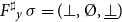 $F^\sharp{}_y\,\sigma = (\bot,\unicode{x00D8},\underline\bot)$
where
$F^\sharp{}_y\,\sigma = (\bot,\unicode{x00D8},\underline\bot)$
where
 $\underline\bot$
is the mapping which assigns
$\underline\bot$
is the mapping which assigns
 $\bot$
to each unknown. For convenience, we make the extra assumption that side effects only occur to unknowns in
$\bot$
to each unknown. For convenience, we make the extra assumption that side effects only occur to unknowns in
 $\textit{leaf}$
.
$\textit{leaf}$
.
A partial post-solution of
 $\mathbb{E}^\sharp$
has to take side effects incurred by the evaluation of the right-hand sides into account. Let
$\mathbb{E}^\sharp$
has to take side effects incurred by the evaluation of the right-hand sides into account. Let
 $\sigma : \mathcal{X}^\sharp\to\mathbb{D}$
and
$\sigma : \mathcal{X}^\sharp\to\mathbb{D}$
and
 $\textit{dom}^\sharp\subseteq\mathcal{X}^\sharp$
. Then we call
$\textit{dom}^\sharp\subseteq\mathcal{X}^\sharp$
. Then we call
 $\textit{dom}^\sharp$
 $(\sigma,\mathbb{E}^\sharp)$
-closed if for all
$(\sigma,\mathbb{E}^\sharp)$
-closed if for all
 $x\in\textit{dom}^\sharp$
and
$x\in\textit{dom}^\sharp$
and
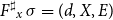 $F^\sharp{}_x\,\sigma = (d,X,E)$
,
$F^\sharp{}_x\,\sigma = (d,X,E)$
,
 $X\subseteq\textit{dom}^\sharp$
and also
$X\subseteq\textit{dom}^\sharp$
and also
 $E\,y\neq\bot$
only for unknowns
$E\,y\neq\bot$
only for unknowns
 $y\in\textit{dom}^\sharp$
. The pair
$y\in\textit{dom}^\sharp$
. The pair
 $(\sigma,\textit{dom}^\sharp)$
is a partial post-solution of
$(\sigma,\textit{dom}^\sharp)$
is a partial post-solution of
 $\mathbb{E}^\sharp$
if
$\mathbb{E}^\sharp$
if
-
1.
$\textit{dom}^\sharp$
is
$(\sigma,\mathbb{E}^\sharp)$
-closed, and -
2. for all
$x\in\textit{dom}^\sharp$
with
$F^\sharp{}_x\,\sigma = (d,X,E)$
,-
(a)
$\sigma\sqsupseteq E$
, and -
(b)
$\sigma\,x\sqsupseteq d$
.
-


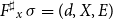


Our goal is to design an extension of the generic local solver
 $\mathbf{TD}_{\mathbf{term}}$
which is able to deal with side-effecting systems of abstract equations. Due to the intertwined narrowing iterations, property (2.b) may be violated. Therefore, consider a pair
$\mathbf{TD}_{\mathbf{term}}$
which is able to deal with side-effecting systems of abstract equations. Due to the intertwined narrowing iterations, property (2.b) may be violated. Therefore, consider a pair
 $(\sigma,\textit{dom}^\sharp)$
satisfying properties (1) and (2.a). Let
$(\sigma,\textit{dom}^\sharp)$
satisfying properties (1) and (2.a). Let
 $\rho:\mathcal{X}^\sharp\to\mathbb{D}$
denote the accumulated side effects of the pair, that is,
$\rho:\mathcal{X}^\sharp\to\mathbb{D}$
denote the accumulated side effects of the pair, that is,
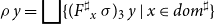 \begin{equation*}\rho\,y = \bigsqcup\{(F^\sharp{}_x\,\sigma)_3\,y\mid x\in\textit{dom}^\sharp\}\end{equation*}
We remark that
 $\rho\,y\neq\bot$
only for unknowns
$\rho\,y\neq\bot$
only for unknowns
 $y\in\textit{dom}^\sharp$
. Let
$y\in\textit{dom}^\sharp$
. Let
 $\mathbb{E}^{\rho}$
denote the system of abstract equations (without side effects) where the right-hand side
$\mathbb{E}^{\rho}$
denote the system of abstract equations (without side effects) where the right-hand side
 $f^\rho_x$
of
$f^\rho_x$
of
 $x\in\mathcal{X}^\sharp$
is given by
$x\in\mathcal{X}^\sharp$
is given by
 \begin{equation*}f^\rho_x\,\sigma'' =\textsf{bind}\,(f^\sharp{}_x\,\sigma''\,(\textbf{fun}\,\_\,\_\to \textsf{return}\,()))\,(\textbf{fun}\,b\to\textsf{return}\,(\rho\,x\sqcup b))\end{equation*}
for
 $\sigma'':\mathcal{X}\to\mathcal{M}(\mathbb{D})$
. This means that all side effects are now ignored, while instead the returned values take the contributions of
$\sigma'':\mathcal{X}\to\mathcal{M}(\mathbb{D})$
. This means that all side effects are now ignored, while instead the returned values take the contributions of
 $\rho$
into account. For the elaborated right-hand side for x and
$\rho$
into account. For the elaborated right-hand side for x and
 $\sigma:\mathcal{X}\to\mathbb{D},$
this means that
$\sigma:\mathcal{X}\to\mathbb{D},$
this means that
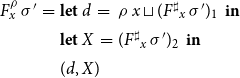 \begin{equation*}\begin{array}{rlll}F^\rho_x\,\sigma' &=& \textbf{let}\;d \;=& \rho\,x\sqcup(F^\sharp{}_x\,\sigma')_1\;\;\textbf{in} \\ & & \textbf{let}\;X \;=& (F^\sharp{}_x\,\sigma')_2\;\;\textbf{in}\\ & & (d,X)\end{array}\end{equation*}
Let
 $\underline\sigma^\rho$
denote the least solution of the lower monotonization of
$\underline\sigma^\rho$
denote the least solution of the lower monotonization of
 $\mathbb{E}^\rho$
. Then, we replace condition (2.b) for
$\mathbb{E}^\rho$
. Then, we replace condition (2.b) for
 $(\sigma,\textit{dom}^\sharp)$
with the condition
$(\sigma,\textit{dom}^\sharp)$
with the condition
(2.b’)
 $\underline\sigma^\rho\,x\sqsubseteq\sigma\,x$
for all
$\underline\sigma^\rho\,x\sqsubseteq\sigma\,x$
for all
 $x\in\textit{dom}^\sharp$
.
$x\in\textit{dom}^\sharp$
.
In this case, we call
 $(\sigma,\textit{dom}^\sharp)$
an improved partial post-condition. The significance of that notion is provided by the next proposition.
$(\sigma,\textit{dom}^\sharp)$
an improved partial post-condition. The significance of that notion is provided by the next proposition.
In the following, we assume that the concrete system
 $\mathbb{E}$
of equations may have side effects, but is monotonic. In that case, it also has for each subset X of unknowns, a unique least partial solution
$\mathbb{E}$
of equations may have side effects, but is monotonic. In that case, it also has for each subset X of unknowns, a unique least partial solution
 $(\sigma,\textit{dom})$
with
$(\sigma,\textit{dom})$
with
 $X\subseteq\textit{dom}$
. For the following proposition, we make the reasonable assumption that the abstract value
$X\subseteq\textit{dom}$
. For the following proposition, we make the reasonable assumption that the abstract value
 $\bot$
only describes an empty set of concrete states, that is,
$\bot$
only describes an empty set of concrete states, that is,
 $\gamma\,\bot = \unicode{x00D8}$
. In an earlier version of this paper, we additionally introduced the restriction that each concrete unknown x is described by at most one unknown
$\gamma\,\bot = \unicode{x00D8}$
. In an earlier version of this paper, we additionally introduced the restriction that each concrete unknown x is described by at most one unknown
 $x^\sharp$
in the abstract. This property, for example, is met for unknowns representing global variables such as g and h in Example 14 – but is violated when partial contexts are used. Removal of the given restriction is now possible due to the parametrization of the description relation
$x^\sharp$
in the abstract. This property, for example, is met for unknowns representing global variables such as g and h in Example 14 – but is violated when partial contexts are used. Removal of the given restriction is now possible due to the parametrization of the description relation
 $\mathrel{\mathcal{R}}$
, that is, the (perhaps) surprising observation that the description relation may not be given before-hand – but is calculated by the analysis itself. We have:
$\mathrel{\mathcal{R}}$
, that is, the (perhaps) surprising observation that the description relation may not be given before-hand – but is calculated by the analysis itself. We have:
Proposition 4. Assume that
 $(\sigma^\sharp,\textit{dom}^\sharp)$
is an improved partial post-solution of
$(\sigma^\sharp,\textit{dom}^\sharp)$
is an improved partial post-solution of
 $\mathbb{E}^\sharp$
with
$\mathbb{E}^\sharp$
with
 $X^\sharp\subseteq\textit{dom}^\sharp$
, and that
$X^\sharp\subseteq\textit{dom}^\sharp$
, and that
 $\mathbb{E} \mathrel{\mathcal{R}_\rho} \mathbb{E}^\sharp$
holds and
$\mathbb{E} \mathrel{\mathcal{R}_\rho} \mathbb{E}^\sharp$
holds and
 $X \mathrel{\mathcal{R}_\rho} X^\sharp$
for some set X of concrete unknowns. Assume further that
$X \mathrel{\mathcal{R}_\rho} X^\sharp$
for some set X of concrete unknowns. Assume further that
 $(\sigma,\textit{dom})$
is the least partial solution of the concrete system with
$(\sigma,\textit{dom})$
is the least partial solution of the concrete system with
 $X\subseteq\textit{dom}$
, Then
$X\subseteq\textit{dom}$
, Then
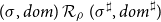 $(\sigma,\textit{dom}) \mathrel{\mathcal{R}_\rho} (\sigma^\sharp,\textit{dom}^\sharp)$
holds.
$(\sigma,\textit{dom}) \mathrel{\mathcal{R}_\rho} (\sigma^\sharp,\textit{dom}^\sharp)$
holds.
Proof. Let
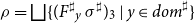 $\rho = \bigsqcup\{(F^\sharp{}_y\,\sigma^\sharp)_3\mid y\in\textit{dom}^\sharp\}$
denote the accumulated side effect corresponding to
$\rho = \bigsqcup\{(F^\sharp{}_y\,\sigma^\sharp)_3\mid y\in\textit{dom}^\sharp\}$
denote the accumulated side effect corresponding to
 $\sigma^\sharp$
. Let
$\sigma^\sharp$
. Let
 $\underline\sigma^\rho$
denote the least solution of the lower monotonization
$\underline\sigma^\rho$
denote the least solution of the lower monotonization
 $\underline{\mathbb{E}^\rho}$
. As in the case without side effects, we proceed by ordinal induction. For each ordinal
$\underline{\mathbb{E}^\rho}$
. As in the case without side effects, we proceed by ordinal induction. For each ordinal
 $\iota$
, we define the corresponding approximation
$\iota$
, we define the corresponding approximation
 $(\sigma{}_\iota,\textit{dom}{}_\iota)$
of
$(\sigma{}_\iota,\textit{dom}{}_\iota)$
of
 $(\sigma,\textit{dom})$
by:
$(\sigma,\textit{dom})$
by:
-
$\sigma{}_0\,x=\unicode{x00D8}$
for all
$x\in\mathcal{X}$
and
$\textit{dom}{}_0=X$
;
-
For each successor ordinal
$\iota'=\iota+1$
,
\begin{equation*} \begin{array}{lll} \sigma{}_{\iota'}\,y &=& (F_y\,\sigma{}_\iota)_1\cup \{(F_z\,\sigma{}_\iota)_3\,y\mid z\in\textit{dom}{}_\iota\} \\ \textit{dom}{}_{\iota'} & = & \textit{dom}{}_\iota\;\cup \bigcup\{(F_y\,\sigma{}_\iota)_2\mid y\in\textit{dom}{}_\iota\}\;\cup\\ & & \{y\mid z\in\textit{dom}{}_\iota,(F_z\,\sigma{}_\iota)_3\,y\neq\unicode{x00D8}\} \end{array} \end{equation*}
-
For each limit ordinal
$\iota'$
,
$\sigma{}_{\iota'}\,y = \bigcup\{\sigma{}_\iota\,y\mid \iota<\iota'\}$
, and
$\textit{dom}{}_{\iota'} = \bigcup\{\textit{dom}{}_\iota\mid \iota<\iota'\}$
.


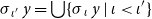
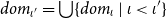
where generally,
 $\sigma{}_{\iota'}\,y=\unicode{x00D8}$
for all
$\sigma{}_{\iota'}\,y=\unicode{x00D8}$
for all
 $y\not\in\textit{dom}{}_{\iota'}$
. Our goal is to prove for each ordinal
$y\not\in\textit{dom}{}_{\iota'}$
. Our goal is to prove for each ordinal
 $\iota'$
, that
$\iota'$
, that
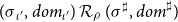 $(\sigma{}_{\iota'},\textit{dom}{}_{\iota'}) \mathrel{\mathcal{R}_\rho} (\sigma^\sharp,\textit{dom}^\sharp)$
holds. This assertion clearly holds for
$(\sigma{}_{\iota'},\textit{dom}{}_{\iota'}) \mathrel{\mathcal{R}_\rho} (\sigma^\sharp,\textit{dom}^\sharp)$
holds. This assertion clearly holds for
 $\iota'=0$
, and also for each limit ordinal
$\iota'=0$
, and also for each limit ordinal
 $\iota'$
, if it holds for each ordinal
$\iota'$
, if it holds for each ordinal
 $\iota<\iota'$
. Therefore, it remains to consider the case of a successor ordinal
$\iota<\iota'$
. Therefore, it remains to consider the case of a successor ordinal
 $\iota'=\iota+1$
. Then, we have by inductive hypothesis, for each
$\iota'=\iota+1$
. Then, we have by inductive hypothesis, for each
 $y\in\textit{dom}{}_\iota$
, there exists some
$y\in\textit{dom}{}_\iota$
, there exists some
 $y^\sharp\in\textit{dom}^\sharp$
with
$y^\sharp\in\textit{dom}^\sharp$
with
 $y \mathrel{\mathcal{R}_\rho} y^\sharp$
, and also
$y \mathrel{\mathcal{R}_\rho} y^\sharp$
, and also
 $\sigma{}_\iota \mathrel{\mathcal{R}_\rho} \sigma^\sharp$
. Since
$\sigma{}_\iota \mathrel{\mathcal{R}_\rho} \sigma^\sharp$
. Since
 $\mathbb{E} \mathrel{\mathcal{R}_\rho} \mathbb{E}^\sharp$
, we have that for each such
$\mathbb{E} \mathrel{\mathcal{R}_\rho} \mathbb{E}^\sharp$
, we have that for each such
 $y^\sharp$
,
$y^\sharp$
,
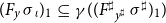 \begin{equation*}\begin{array}{lll}(F_y\,\sigma{}_\iota)_1&\subseteq&\gamma((F^\sharp{}_{y^\sharp}\,\sigma^\sharp)_1)\end{array}\end{equation*}
and thus likewise,
 \begin{equation*}\begin{array}{lll}(F_y\,\sigma{}_\iota)_1&\subseteq&\gamma((\underline F^\sharp{}_{y^\sharp}\,\sigma^\sharp)_1) \\ &\subseteq&\gamma(\underline\sigma^\rho\,y^\sharp) \\ &\subseteq&\gamma(\underline\sigma^\sharp\,y^\sharp)\end{array}\end{equation*}
furthermore for unknowns
 $z\in\textit{dom}{}_\iota$
and
$z\in\textit{dom}{}_\iota$
and
 $z^\sharp\in\textit{dom}^\sharp$
with
$z^\sharp\in\textit{dom}^\sharp$
with
 $z \mathrel{\mathcal{R}_\rho} z^\sharp$
,
$z \mathrel{\mathcal{R}_\rho} z^\sharp$
,
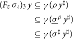 \begin{equation*}\begin{array}{lll}(F_z\,\sigma{}_\iota)_3\,y &\subseteq& \gamma(\rho\,y^\sharp) \\ &\subseteq& \gamma(\underline\sigma^\rho\,y^\sharp) \\ &\subseteq& \gamma(\sigma^\sharp\,y^\sharp)\end{array}\end{equation*}
Altogether therefore,
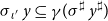 \begin{equation*}\sigma{}_{\iota'}\,y \subseteq \gamma(\sigma^\sharp\,y^\sharp)\end{equation*}
which we wanted to prove. It remains to prove that also
 $\textit{dom}{}_{\iota'} \mathrel{\mathcal{R}_\rho} \textit{dom}^\sharp$
holds. By induction hypothesis for
$\textit{dom}{}_{\iota'} \mathrel{\mathcal{R}_\rho} \textit{dom}^\sharp$
holds. By induction hypothesis for
 $\iota$
,
$\iota$
,
 $\textit{dom}{}_\iota \mathrel{\mathcal{R}_\rho} \textit{dom}^\sharp$
holds. Since
$\textit{dom}{}_\iota \mathrel{\mathcal{R}_\rho} \textit{dom}^\sharp$
holds. Since
 $\mathbb{E} \mathrel{\mathcal{R}_\rho} \mathbb{E}^\sharp$
, also
$\mathbb{E} \mathrel{\mathcal{R}_\rho} \mathbb{E}^\sharp$
, also
 $(F_y\,\sigma{}_\iota)_2 \mathrel{\mathcal{R}_\rho} (F^\sharp{}_{y^\sharp}\,\sigma^\sharp)_2$
holds. Moreover,
$(F_y\,\sigma{}_\iota)_2 \mathrel{\mathcal{R}_\rho} (F^\sharp{}_{y^\sharp}\,\sigma^\sharp)_2$
holds. Moreover,
 $(F_z\,\sigma{}_\iota)_3\,y\neq\unicode{x00D8}$
implies that
$(F_z\,\sigma{}_\iota)_3\,y\neq\unicode{x00D8}$
implies that
 $\rho\,y^\sharp\neq\bot$
whenever
$\rho\,y^\sharp\neq\bot$
whenever
 $y \mathrel{\mathcal{R}_\rho} y^\sharp$
holds. But then there must be some
$y \mathrel{\mathcal{R}_\rho} y^\sharp$
holds. But then there must be some
 $z^\sharp$
with
$z^\sharp$
with
 $(F^\sharp{}_{z^\sharp}\,\sigma^\sharp)_3\,y^\sharp\neq\bot$
. Accordingly,
$(F^\sharp{}_{z^\sharp}\,\sigma^\sharp)_3\,y^\sharp\neq\bot$
. Accordingly,
 $y^\sharp\in\textit{dom}^\sharp$
. This completes the proof.
$y^\sharp\in\textit{dom}^\sharp$
. This completes the proof.
In light of Proposition 4, it therefore suffices to design algorithms for computing improved partial post-solutions of the abstract system starting from a given set of abstract unknowns. For that, we assume that the abstract system
 $\mathbb{E}^\sharp$
provides us for each abstract unknown
$\mathbb{E}^\sharp$
provides us for each abstract unknown
 $x^\sharp\in\mathcal{X}^\sharp$
, with a right-hand side function
$x^\sharp\in\mathcal{X}^\sharp$
, with a right-hand side function
 $f^\sharp{}_{x^\sharp}$
of type
$f^\sharp{}_{x^\sharp}$
of type
 $(\mathcal{X}\to\mathcal{M}(\mathbb{D}))\to(\mathcal{X}\to\mathbb{D}\to\mathcal{M}(\bullet))\to\mathcal{M}(\mathbb{D})$
for every monad
$(\mathcal{X}\to\mathcal{M}(\mathbb{D}))\to(\mathcal{X}\to\mathbb{D}\to\mathcal{M}(\bullet))\to\mathcal{M}(\mathbb{D})$
for every monad
 $\mathcal{M}$
. As before, the solver state is maintained in mutable data structures. Therefore, the algorithm assumes right-hand side functions to have the OCaml type
$\mathcal{M}$
. As before, the solver state is maintained in mutable data structures. Therefore, the algorithm assumes right-hand side functions to have the OCaml type
 $(\mathcal{X}\to\mathbb{D})\to(\mathcal{X}\to\mathbb{D}\to\bullet)\to\mathbb{D}$
. As an extension of
$(\mathcal{X}\to\mathbb{D})\to(\mathcal{X}\to\mathbb{D}\to\bullet)\to\mathbb{D}$
. As an extension of
 $\mathbf{TD}_{\mathbf{term}}$
, we introduce the solver
$\mathbf{TD}_{\mathbf{term}}$
, we introduce the solver
 $\mathbf{TD}_{\mathbf{side}}$
. In order to decide whether or not the different side effects to a leaf unknown y should be combined by the join operator
$\mathbf{TD}_{\mathbf{side}}$
. In order to decide whether or not the different side effects to a leaf unknown y should be combined by the join operator
 $\sqcup$
or widening, the solver now maintains an additional data structure to record for each unknown y the set of unknowns from which it has received a side effect.
$\sqcup$
or widening, the solver now maintains an additional data structure to record for each unknown y the set of unknowns from which it has received a side effect.
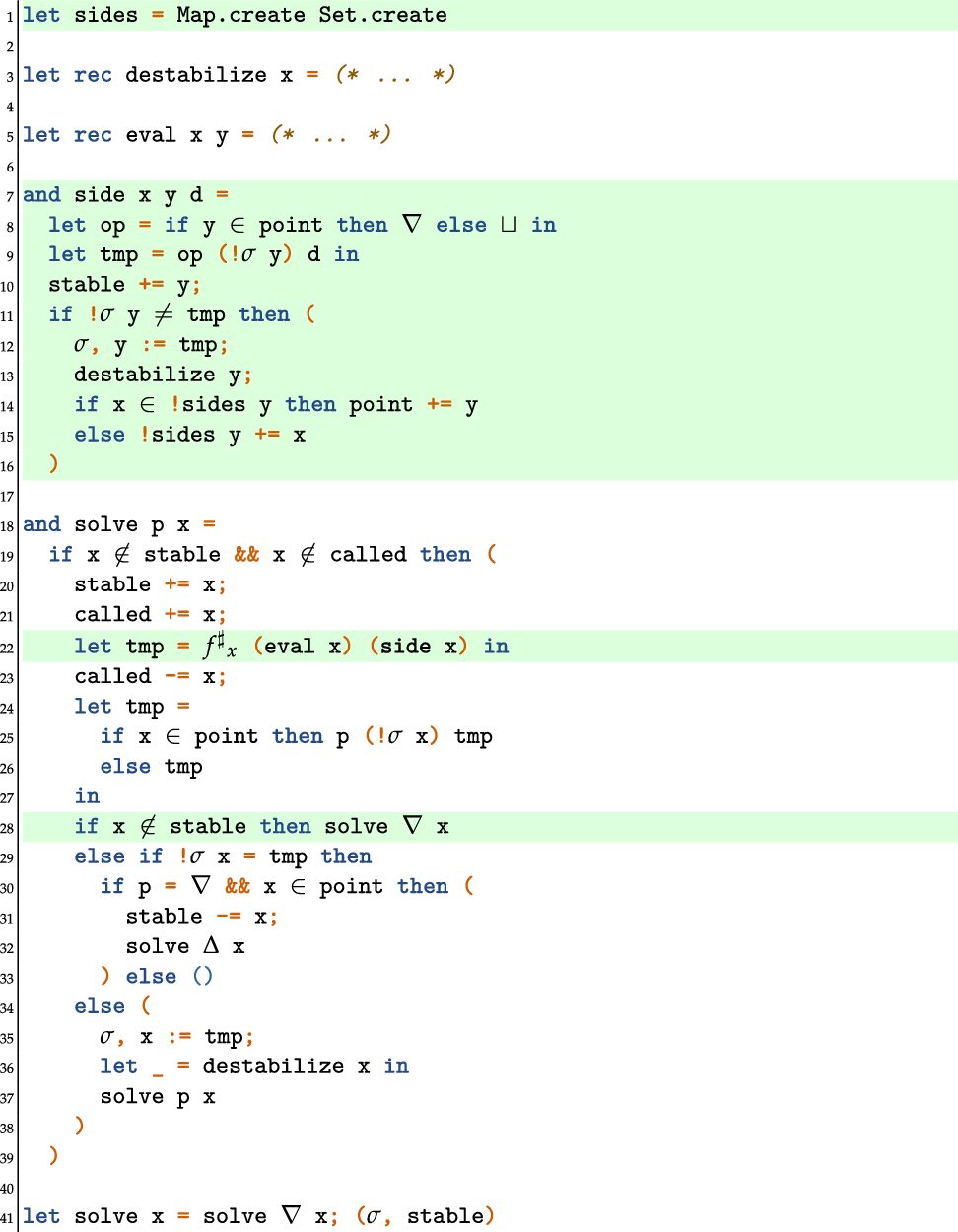
The functions
 $\textsf{destabilize}$
and
$\textsf{destabilize}$
and
 $\textsf{eval}$
have not been changed. New, however, is the function
$\textsf{eval}$
have not been changed. New, however, is the function
 $\textsf{side}$
. A call
$\textsf{side}$
. A call
 $\textsf{side}\;x\;y\;d$
realizes the side effect from the unknown x onto the unknown y by combining the old value for y in
$\textsf{side}\;x\;y\;d$
realizes the side effect from the unknown x onto the unknown y by combining the old value for y in
 $\sigma$
with the new contribution d. If y is marked as a widening point, the value is combined using the widening operator, otherwise using the join operator. Generally, y is marked as stable. If the result is different from the old value for y, then the value of y in
$\sigma$
with the new contribution d. If y is marked as a widening point, the value is combined using the widening operator, otherwise using the join operator. Generally, y is marked as stable. If the result is different from the old value for y, then the value of y in
 $\sigma$
is updated, and all influenced unknowns are destabilized by means of the call
$\sigma$
is updated, and all influenced unknowns are destabilized by means of the call
 $\textsf{destabilize}\;y$
.
$\textsf{destabilize}\;y$
.
In order to decide whether y should be included into the set
 $\textit{point}$
, the algorithm maintains for each (leaf) unknown y’ the set
$\textit{point}$
, the algorithm maintains for each (leaf) unknown y’ the set
 $\textit{sides}\,y'$
of all unknowns whose evaluations so far have led to an increase of the value of y’. Thus, if the current contribution d is not subsumed by
$\textit{sides}\,y'$
of all unknowns whose evaluations so far have led to an increase of the value of y’. Thus, if the current contribution d is not subsumed by
 $\sigma\,y$
and x is already contained in
$\sigma\,y$
and x is already contained in
 $\textit{sides}\,y$
, then y is added to the set
$\textit{sides}\,y$
, then y is added to the set
 $\textit{point}$
.
$\textit{point}$
.
We remark that the call
 $\textsf{side}\;x\;y\;d$
may update the value of the leaf unknown y, but does not itself call the procedure solve. Accordingly, it removes those unknowns from stable whose latest values have been computed based on the out-dated assumption on y.
$\textsf{side}\;x\;y\;d$
may update the value of the leaf unknown y, but does not itself call the procedure solve. Accordingly, it removes those unknowns from stable whose latest values have been computed based on the out-dated assumption on y.
Finally, the main function
 $\textsf{solve}$
is adapted to take side effects into account. This means that the evaluation of the right-hand side for an unknown x must now take the partial application
$\textsf{solve}$
is adapted to take side effects into account. This means that the evaluation of the right-hand side for an unknown x must now take the partial application
 $\textsf{side}\,x$
as second argument. In presence of side effects, we may no longer assume that, after evaluation of
$\textsf{side}\,x$
as second argument. In presence of side effects, we may no longer assume that, after evaluation of
 $f^\sharp{}_x\,(\textsf{eval}\,x)\,(\textsf{side}\,x)$
, the left-hand side x is necessarily contained in
$f^\sharp{}_x\,(\textsf{eval}\,x)\,(\textsf{side}\,x)$
, the left-hand side x is necessarily contained in
 $\textit{stable}$
. Destabilization of x could only have been caused due to some side effect during solving of subsequent unknowns. In this case, we call
$\textit{stable}$
. Destabilization of x could only have been caused due to some side effect during solving of subsequent unknowns. In this case, we call
 $\textsf{solve}\,\nabla\,x$
– no matter whether we had already reached the narrowing iteration for x or not.
$\textsf{solve}\,\nabla\,x$
– no matter whether we had already reached the narrowing iteration for x or not.
Example 17. Consider, for example, the abstract equation system from Example 16 for the program from Example 14.
Starting
 $\mathbf{TD}_{\mathbf{side}}$
for the unknown
$\mathbf{TD}_{\mathbf{side}}$
for the unknown
 $\textsf{main}$
in an initial solver state
$\textsf{main}$
in an initial solver state
 $s_0$
where all data structures are empty, will first produce side effects to g,h and record that increasing side effects have occurred from main. Then the evaluation of the unknown f is triggered.
$s_0$
where all data structures are empty, will first produce side effects to g,h and record that increasing side effects have occurred from main. Then the evaluation of the unknown f is triggered.
Evaluating the computation tree
 $t_f$
will query g (which is already found stable) and result in another side effect to h. None of these unknowns so far is put into the set point.
$t_f$
will query g (which is already found stable) and result in another side effect to h. None of these unknowns so far is put into the set point.
Continuing with the evaluation of the computation tree
 $t_{\textsf{main}}$
will produce another side effect onto g. Since the value of g in
$t_{\textsf{main}}$
will produce another side effect onto g. Since the value of g in
 $\sigma$
is again modified, g is now put into the set
$\sigma$
is again modified, g is now put into the set
 $\textit{point}$
. Furthermore,
$\textit{point}$
. Furthermore,
 $\textsf{destabilize}\,g$
is called – which will remove f as well as
$\textsf{destabilize}\,g$
is called – which will remove f as well as
 $\textsf{main}$
from the set stable. At that point,
$\textsf{main}$
from the set stable. At that point,
 $\textsf{main}$
is still contained in called. This implies that
$\textsf{main}$
is still contained in called. This implies that
 $\textsf{solve}\,\nabla\,\textsf{main}$
is called again.
$\textsf{solve}\,\nabla\,\textsf{main}$
is called again.
The second round of solving with
 $\nabla$
, though, will only update the values of h (recording at h an increasing contribution from f) and
$\nabla$
, though, will only update the values of h (recording at h an increasing contribution from f) and
 $\textsf{main}$
in
$\textsf{main}$
in
 $\sigma$
to [0,1] and [0,0], respectively, while leaving all unknowns in stable. Also, the subsequent call
$\sigma$
to [0,1] and [0,0], respectively, while leaving all unknowns in stable. Also, the subsequent call
 $\textsf{destabilize}\,\textsf{main}$
will not remove
$\textsf{destabilize}\,\textsf{main}$
will not remove
 $\textsf{main}$
from stable, and the iteration terminates with
$\textsf{main}$
from stable, and the iteration terminates with
 \begin{equation*}\sigma = \{g\mapsto[0,1],h\mapsto[0,1],f\mapsto[0,0],\textsf{main}\mapsto[0,0]\}\end{equation*}
We remark that in the preliminary version of the solver
 $\mathbf{TD}_{\mathbf{side}}$
in Seidl and Vogler (Reference Seidl, Vogler and Thiemann2018), the fresh values for globals are always combined with the corresponding old values by means of widening. This has been improved in the present version of the solver where widening for globals is restricted only to those globals which have been put into point.
$\mathbf{TD}_{\mathbf{side}}$
in Seidl and Vogler (Reference Seidl, Vogler and Thiemann2018), the fresh values for globals are always combined with the corresponding old values by means of widening. This has been improved in the present version of the solver where widening for globals is restricted only to those globals which have been put into point.
In order to reason about termination and soundness of
 $\mathbf{TD}_{\mathbf{side}}$
, we extend the notion of consistency as introduced in Section 5 appropriately. We now call a solver state
$\mathbf{TD}_{\mathbf{side}}$
, we extend the notion of consistency as introduced in Section 5 appropriately. We now call a solver state
 $s=(\sigma,\textit{infl},\textit{sides},\textit{stable},\textit{called},\textit{point})$
consistent if
$s=(\sigma,\textit{infl},\textit{sides},\textit{stable},\textit{called},\textit{point})$
consistent if
-
1. for all
$x\in(\textit{stable}\setminus\textit{called})$
, -
(a) for all
$y \in (F^\sharp{}_x\sigma)_2$
,
$y\in(\textit{stable}\,\cup\,\textit{called})$
and
$x\in\textit{infl}\,y$
holds; -
(b) for all y with
$(F^\sharp{}_x\sigma)_3\,y\neq\bot$
,
$(F^\sharp{}_x\sigma)_3\,y\sqsubseteq\sigma\,y$
; -
2. for each
$x\not\in(\textit{stable}\,\cup\,\textit{called})$
,
$\textit{infl}\,x=\unicode{x00D8}$
.


With this modified definition, the invariant for destabilize from Section 5 essentially remains the same, while the invariants for solve and eval must be refined.
Each call
 $\textsf{solve}\,p\,x$
encountered during the evaluation of the initial call, starts in a consistent solver state
$\textsf{solve}\,p\,x$
encountered during the evaluation of the initial call, starts in a consistent solver state
 $s=(\sigma,\textit{infl},\textit{sides},\textit{stable},\textit{called},\textit{point})$
. Upon its termination, a solver state
$s=(\sigma,\textit{infl},\textit{sides},\textit{stable},\textit{called},\textit{point})$
. Upon its termination, a solver state
 $s'=(\sigma',\textit{infl}',\textit{sides}',\textit{stable}',\textit{called}',\textit{point}')$
is attained such that
$s'=(\sigma',\textit{infl}',\textit{sides}',\textit{stable}',\textit{called}',\textit{point}')$
is attained such that
 $s = s'$
when
$s = s'$
when
 $x\in\textit{stable}\cup\textit{called}$
. If
$x\in\textit{stable}\cup\textit{called}$
. If
 $x\not\in\textit{called}\cup\textit{stable}$
, the following holds:
$x\not\in\textit{called}\cup\textit{stable}$
, the following holds:
-
(1). s’ is again consistent;
-
(2).
$\textit{called}'=\textit{called}$
where
$\sigma'\,y=\sigma\,y$
for all
$y\in\textit{called}$
; -
(3).
$\textit{sides}\,y\subseteq\textit{sides}'\,y$
for all y, and
$\textit{point}\subseteq\textit{point}'$
; -
(4).
$x\in\textit{stable}'$
.


In particular, the set of stable unknowns is not necessarily monotonically increasing.
Each call
 $\textsf{eval}\,x\,y$
encountered during the evaluation, starts in a consistent state
$\textsf{eval}\,x\,y$
encountered during the evaluation, starts in a consistent state
 $s=(\sigma,\textit{infl},\textit{sides},\textit{stable},\textit{called},\textit{point})$
where
$s=(\sigma,\textit{infl},\textit{sides},\textit{stable},\textit{called},\textit{point})$
where
 $x\in\textit{called}$
(no longer necessarily also in stable). Upon its termination, a solver state
$x\in\textit{called}$
(no longer necessarily also in stable). Upon its termination, a solver state
 $s'=(\sigma',\textit{infl}',\textit{sides}',\textit{stable}',\textit{called}',\textit{point}')$
is attained such that
$s'=(\sigma',\textit{infl}',\textit{sides}',\textit{stable}',\textit{called}',\textit{point}')$
is attained such that
-
(1). s’ is again consistent;
-
(2).
$\textit{called}'=\textit{called}$
where
$\sigma'\,y'=\sigma\,y'$
for all
$y'\in\textit{called}$
; -
(3).
$\textit{sides}\,y'\subseteq\textit{sides}'\,y'$
for all y’, and
$\textit{point}\subseteq\textit{point}'$
; -
(4). If
$y\in\textit{stable}\cup\textit{called}$
, then-
$\sigma' = \sigma$
,
$\textit{sides}' =\textit{sides}$
,
$\textit{stable}'=\textit{stable}$
, and
$\textit{point}' = \textit{point}$
if
$y\not\in\textit{called}$
whereas
$\textit{point}'=\textit{point}\cup\{y\}$
if
$y\in\textit{called}$
;
-
$\textit{infl}'\,y'=\textit{infl}\,y'$
for all
$y'\neq y$
, and
-
$\textit{infl}'\,y= \textit{infl}\,y\cup\{x\}$
;
-
-
5.
$y\in\textit{stable}'$
,
$x\in\textit{infl}'\,y$
, and the value
$\sigma'\,y$
is returned.


In particular upon termination of
 $\textsf{eval}\,x\,y$
, we are also no longer guaranteed that
$\textsf{eval}\,x\,y$
, we are also no longer guaranteed that
 $x\in\textit{stable}'$
.
$x\in\textit{stable}'$
.
Each call
 $\textsf{side}\,x\,y\,d$
encountered during the evaluation, starts in a consistent state
$\textsf{side}\,x\,y\,d$
encountered during the evaluation, starts in a consistent state
 $s=(\sigma,\textit{infl},\textit{sides},\textit{stable},\textit{called},\textit{point})$
where
$s=(\sigma,\textit{infl},\textit{sides},\textit{stable},\textit{called},\textit{point})$
where
 $x\in\textit{called}$
. Upon its termination, a solver state
$x\in\textit{called}$
. Upon its termination, a solver state
 $s'=(\sigma',\textit{infl}',\textit{sides}',\textit{stable}',\textit{called}',\textit{point}')$
is attained such that
$s'=(\sigma',\textit{infl}',\textit{sides}',\textit{stable}',\textit{called}',\textit{point}')$
is attained such that
 $s = s'$
whenever
$s = s'$
whenever
 $d\sqsubseteq\sigma\,y$
. Otherwise,
$d\sqsubseteq\sigma\,y$
. Otherwise,
-
(1). s’ is again consistent where
$\textit{called}'=\textit{called}$
; -
(2).
$\textit{sides}'\,y = \textit{sides}\,y\cup\{x\}$
, and
$\textit{sides}\,y'=\textit{sides}'\,y'$
for all
$y'\neq y$
; -
(3). If
$x\in\textit{sides}\,y$
then
$\textit{point}' = \textit{point}\cup\{y\}$
, and
$\textit{point}' = \textit{point}$
otherwise; -
(4).
$\sigma'\,y\sqsupseteq \sigma\,y\sqcup d$
, and
$\sigma\,y'=\sigma'\,y'$
for all
$y'\neq y$
; -
(5).
$y\in\textit{stable}'$
where
$\textit{infl}'$
and
$\textit{stable}'$
are obtained from
$\textit{infl}$
and
$\textit{stable}$
by destabilizing y, that is, for all y’,
$\textit{infl}'\,y'$
either equals
$\unicode{x00D8}$
or
$\textit{infl}\,y'$
where
$\textit{infl}'$
and
$\textit{stable}'$
are maximal so that s’ is consistent while
$\textit{infl}'\,y=\unicode{x00D8}$
and
$\textit{infl}\,y\cap\textit{stable}'=\unicode{x00D8}$
.


Given that the number of unknowns encountered during the evaluation of the right-hand side is finite, let us first assume that only finitely many calls
 $\textsf{side}\,x\,y\,d$
ever will result in a modification of
$\textsf{side}\,x\,y\,d$
ever will result in a modification of
 $\sigma$
. Once within the iteration on some x,
$\sigma$
. Once within the iteration on some x,
 $\sigma$
is no longer modified due to side effects; however, the same invariants as for the non-side-effecting solver
$\sigma$
is no longer modified due to side effects; however, the same invariants as for the non-side-effecting solver
 $\mathbf{TD}_{\mathbf{term}}$
apply – allowing us thus to deduce that each encountered call to solve will necessarily terminate. Now assume for a contradiction, that for some consistent solver state, the evaluation of
$\mathbf{TD}_{\mathbf{term}}$
apply – allowing us thus to deduce that each encountered call to solve will necessarily terminate. Now assume for a contradiction, that for some consistent solver state, the evaluation of
 $\textsf{solve}\,p\,x$
results in an infinite number of updates to leaf unknowns, say from set G. From some point on then all leaf unknowns y which have been added to
$\textsf{solve}\,p\,x$
results in an infinite number of updates to leaf unknowns, say from set G. From some point on then all leaf unknowns y which have been added to
 $\textit{point}$
will not change anymore. In particular, none of the unknowns from G has been added to
$\textit{point}$
will not change anymore. In particular, none of the unknowns from G has been added to
 $\textit{point}$
. Then, there must exist some unknown x’ and some unknown
$\textit{point}$
. Then, there must exist some unknown x’ and some unknown
 $g\in G$
so that an infinite sequence of calls
$g\in G$
so that an infinite sequence of calls
 $\textsf{solve}\,p_i\,x'$
is encountered for consistent solver states
$\textsf{solve}\,p_i\,x'$
is encountered for consistent solver states
 $s_i$
immediately before these calls where during the evaluation of the right-hand side of x’ in each of these calls, a side effect to g occurs which results in a change to the value of g.
$s_i$
immediately before these calls where during the evaluation of the right-hand side of x’ in each of these calls, a side effect to g occurs which results in a change to the value of g.
After the first call, however, x’ necessarily will be contained in the set sides y, that is, is contained in sides y at states
 $s_i$
for all
$s_i$
for all
 $i\geq 2$
. This means that g is contained in the set
$i\geq 2$
. This means that g is contained in the set
 $\textit{point}$
after the second call – in contradiction to our assumption. We therefore obtain:
$\textit{point}$
after the second call – in contradiction to our assumption. We therefore obtain:
Theorem 5. Let
 $\mathbb{E}^\sharp$
denote an arbitrary system of abstract equations, and
$\mathbb{E}^\sharp$
denote an arbitrary system of abstract equations, and
 $x_0\in\mathcal{X}^\sharp$
is the unknown of interest. Assume that initially the sets
$x_0\in\mathcal{X}^\sharp$
is the unknown of interest. Assume that initially the sets
 $\textit{called}$
and
$\textit{called}$
and
 $\textit{stable}$
are empty, and likewise,
$\textit{stable}$
are empty, and likewise,
 $\textit{infl}$
maps each unknown to the empty set. Then, the call
$\textit{infl}$
maps each unknown to the empty set. Then, the call
 $\textsf{solve}\,x_0$
of solver
$\textsf{solve}\,x_0$
of solver
 $\mathbf{TD}_{\mathbf{side}}$
will always terminate, as long as only finitely many unknowns are encountered.
$\mathbf{TD}_{\mathbf{side}}$
will always terminate, as long as only finitely many unknowns are encountered.
Likewise, we can adapt the proof of Theorem 2 for the case of no side effects to obtain:
Theorem 6. Each call
 $\textsf{solve}\,\nabla\,x$
encountered during the evaluation of the call
$\textsf{solve}\,\nabla\,x$
encountered during the evaluation of the call
 $\textsf{solve}\,\,x_0$
starting in a saturated solver state
$\textsf{solve}\,\,x_0$
starting in a saturated solver state
 $s=(\sigma,\textit{infl},\textit{stable},\textit{called},\textit{point})$
, results upon termination, in a solver state
$s=(\sigma,\textit{infl},\textit{stable},\textit{called},\textit{point})$
, results upon termination, in a solver state
 $s'=(\sigma',\textit{infl}',\textit{stable}',\textit{called}',\textit{point}')$
which is again saturated where additionally
$s'=(\sigma',\textit{infl}',\textit{stable}',\textit{called}',\textit{point}')$
which is again saturated where additionally
 $x\in\textit{stable}'$
.
$x\in\textit{stable}'$
.
The proof is based on a variant of the proof of Theorem 2. Taking into account that from some point in evaluation on, only calls
 $\textsf{solve}\,p\,x$
occur where
$\textsf{solve}\,p\,x$
occur where
 $\sigma\,y$
does no longer change for any encountered unknown
$\sigma\,y$
does no longer change for any encountered unknown
 $y\in\textit{leaf}$
via side effects, we obtain as a corollary:
$y\in\textit{leaf}$
via side effects, we obtain as a corollary:
Corollary 5. Assume that
 $\mathbb{E}^\sharp$
is a system of abstract equations with side effects and
$\mathbb{E}^\sharp$
is a system of abstract equations with side effects and
 $x_0$
is an unknown of
$x_0$
is an unknown of
 $\mathbb{E}^\sharp$
. Assume that the sets
$\mathbb{E}^\sharp$
. Assume that the sets
 $\textit{stable}$
and
$\textit{stable}$
and
 $\textit{called}$
are empty, and
$\textit{called}$
are empty, and
 $\textit{infl}$
maps each unknown to
$\textit{infl}$
maps each unknown to
 $\unicode{x00D8}$
. Assume that the top-level call
$\unicode{x00D8}$
. Assume that the top-level call
 $\textsf{solve}\,x_0$
is evaluated by
$\textsf{solve}\,x_0$
is evaluated by
 $\mathbf{TD}_{\mathbf{side}}$
for
$\mathbf{TD}_{\mathbf{side}}$
for
 $\mathbb{E}^\sharp$
. Let
$\mathbb{E}^\sharp$
. Let
 $\sigma$
and
$\sigma$
and
 $\textit{stable}$
denote the values of these data structures after termination. Then
$\textit{stable}$
denote the values of these data structures after termination. Then
 $x_0\in\textit{stable}$
, and
$x_0\in\textit{stable}$
, and
 $(\sigma,\textit{stable})$
is an improved partial post-solution of
$(\sigma,\textit{stable})$
is an improved partial post-solution of
 $\mathbb{E}^\sharp$
.
$\mathbb{E}^\sharp$
.
10. Experimental Evaluation
We implemented the presented solvers within the analysis framework Goblint.Footnote 1 In particular, we also realized a solver TDspaceτ+side which combines the optimization for space with side effects (see Appendix C for this solver). The solvers were evaluated on the SPECint benchmark suiteFootnote 2 consisting of not too small real-world C programs (1600–34,000 LOC after preprocessing). The programs 433.milc, 470.lbm, and 482.sphinx are part of the CFP2006 benchmark suite.Footnote 3 Furthermore, the following C programs were analyzed: duff-0.5,Footnote 4 ent-2008-01-28,Footnote 5 figlet-2.2.5,Footnote 6 maradns-1.4.06,Footnote 7 wget-1.12, Footnote 8 and some programs from the coreutilsFootnote 9 package. The analyzed program wget-1.12 is the largest one with around 77,000 LOC. However, lines of code is not a good metric for complexity since there might be a lot of unused definitions from header files, and on the other hand many revisited lines due to loops and function calls. The most complex program by number of unknowns is 458.sjeng with 322,321 unknowns but only 17,336 LOC. On top of a basic analysis of pointers and strings, we put an interval analysis of integer variables. By this, we chose the simplest meaningful setup where widening and narrowing is required. Clearly, at the expense of worse scalability, more complicated abstract domains could be tried within the same analysis framework. The benchmark programs were analyzed with full context-sensitivity of local data while globals were treated flow-insensitively. For programs with recursive function calls, the functions will be analyzed for more and more contexts which may lead to excessively long analysis times, stack overflows, or exhaustion of memory. We added an extra option that keeps the contexts for currently called functions for each unknown and widens the context for recursive calls. This can be seen as an abstraction of the call stack with a partial map from function names to abstract calling contexts. This partial map itself is not included into the context, but propagated via side effect to the entry points of the called functions. The analysis of the following programs only terminated with this widening on contexts enabled (these are suffixed with * below in figures and text): 458.sjeng, 482.sphinx, duff-0.5, maradns-1.4.06, coreutils-8.13-ls, coreutils-8.13-sort. The analysis of the following programs did not terminate within the given timeout of eight hours: 400.perlbench, 445.gobmk, wget-1.12. Our hypothesis is that widening on contexts for these programs still results in too many intermediate contexts. All benchmarks ran with an increased stack space of 48 MB (ulimit -Ss 49152).
Figure 3 compares the solvers TDspaceτ+side and
 $\mathbf{TD}_{\mathbf{side}}$
in terms of space and time. As a metric for space, we choose the total number of unknowns (i.e., occurring pairs of program points and contexts), and for time the total number of evaluations of right-hand sides of corresponding unknowns. Solver
$\mathbf{TD}_{\mathbf{side}}$
in terms of space and time. As a metric for space, we choose the total number of unknowns (i.e., occurring pairs of program points and contexts), and for time the total number of evaluations of right-hand sides of corresponding unknowns. Solver
 $\mathbf{TD}_{\mathbf{side}}$
requires more than four times as many unknowns as the solver TDspaceτ+side. As expected, the price to be paid by solver TDspaceτ+side for the fewer unknowns is an increase in the number of evaluations of right-hand sides. In practice, the CPU times and memory usage are of interest. For our experiments, we used an Intel Xeon E3–1270 v3 (3.50 GHz) with 32 GB of RAM.
$\mathbf{TD}_{\mathbf{side}}$
requires more than four times as many unknowns as the solver TDspaceτ+side. As expected, the price to be paid by solver TDspaceτ+side for the fewer unknowns is an increase in the number of evaluations of right-hand sides. In practice, the CPU times and memory usage are of interest. For our experiments, we used an Intel Xeon E3–1270 v3 (3.50 GHz) with 32 GB of RAM.
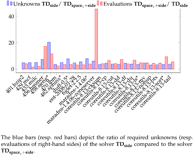
Figure 3. Performance of TDspaceτ+side vs.
 $\mathbf{TD}_{\mathbf{side}}$
.
$\mathbf{TD}_{\mathbf{side}}$
.
Table 1 shows the number of unknowns, evaluations, the CPU time, and peak memory usage for
 $\mathbf{TD}_{\mathbf{side}}$
(left columns) and TDspaceτ+side (right columns). The maximum values for each column are bold. In the benchmark column, coreutils has been shortened to cu, as well as zoneserver to zs. The run times roughly correlate with the number of required evaluations of right-hand sides. Concerning memory usage, TDspaceτ+side was 69% of
$\mathbf{TD}_{\mathbf{side}}$
(left columns) and TDspaceτ+side (right columns). The maximum values for each column are bold. In the benchmark column, coreutils has been shortened to cu, as well as zoneserver to zs. The run times roughly correlate with the number of required evaluations of right-hand sides. Concerning memory usage, TDspaceτ+side was 69% of
 $\mathbf{TD}_{\mathbf{side}}$
on average with widening of contexts enabled, and 92% for benchmarks that ran without widening of contexts. The minimum memory usage was around 29 MB which can be seen as the overhead of the rest of the analyzer and the garbage collector. The memory saving gets more noticeable with an increasing number of unknowns. The biggest benchmarks 458.sjeng* and maradns-1.4.06* only consumed 43% and 69% of memory compared to
$\mathbf{TD}_{\mathbf{side}}$
on average with widening of contexts enabled, and 92% for benchmarks that ran without widening of contexts. The minimum memory usage was around 29 MB which can be seen as the overhead of the rest of the analyzer and the garbage collector. The memory saving gets more noticeable with an increasing number of unknowns. The biggest benchmarks 458.sjeng* and maradns-1.4.06* only consumed 43% and 69% of memory compared to
 $\mathbf{TD}_{\mathbf{side}}$
. We have not profiled how efficiently intermediate values can be freed by the garbage collector. The results without widening of contexts give an indication how TDspaceτ+side could be useful for bigger benchmarks: for maradns-1.4.06* it calculated 25,755 widening points, whereas
$\mathbf{TD}_{\mathbf{side}}$
. We have not profiled how efficiently intermediate values can be freed by the garbage collector. The results without widening of contexts give an indication how TDspaceτ+side could be useful for bigger benchmarks: for maradns-1.4.06* it calculated 25,755 widening points, whereas
 $\mathbf{TD}_{\mathbf{side}}$
only managed to calculate 4797 widening points before both failed with a stack overflow with 3.15 GB and 6.23 GB peak memory usage, respectively.
$\mathbf{TD}_{\mathbf{side}}$
only managed to calculate 4797 widening points before both failed with a stack overflow with 3.15 GB and 6.23 GB peak memory usage, respectively.
Table 1. Performance of
 $\mathbf{TD}_{\mathbf{side}}$
and TDspaceτ+side
$\mathbf{TD}_{\mathbf{side}}$
and TDspaceτ+side

Another important question is how the
 $\textbf{TD}_{\unicode{x29C4}}$
solver, that is the version of the TD solver equipped with the warrowing operator as in Apinis et al. (Reference Apinis, Seidl, Vojdani, Probst, Hankin and Hansen2016) and enhanced with our novel treatment of side effects, compares with the solver
$\textbf{TD}_{\unicode{x29C4}}$
solver, that is the version of the TD solver equipped with the warrowing operator as in Apinis et al. (Reference Apinis, Seidl, Vojdani, Probst, Hankin and Hansen2016) and enhanced with our novel treatment of side effects, compares with the solver
 $\mathbf{TD}_{\mathbf{side}}$
in terms of run time and precision. Interestingly, we found that
$\mathbf{TD}_{\mathbf{side}}$
in terms of run time and precision. Interestingly, we found that
 $\mathbf{TD}_{\mathbf{side}}$
on average runs 25% longer and gives the same results, that is, no differences in precision. The run times of the two variants are shown in Figure 4 in absolute numbers as well as in Figure 5 in relation.
$\mathbf{TD}_{\mathbf{side}}$
on average runs 25% longer and gives the same results, that is, no differences in precision. The run times of the two variants are shown in Figure 4 in absolute numbers as well as in Figure 5 in relation.
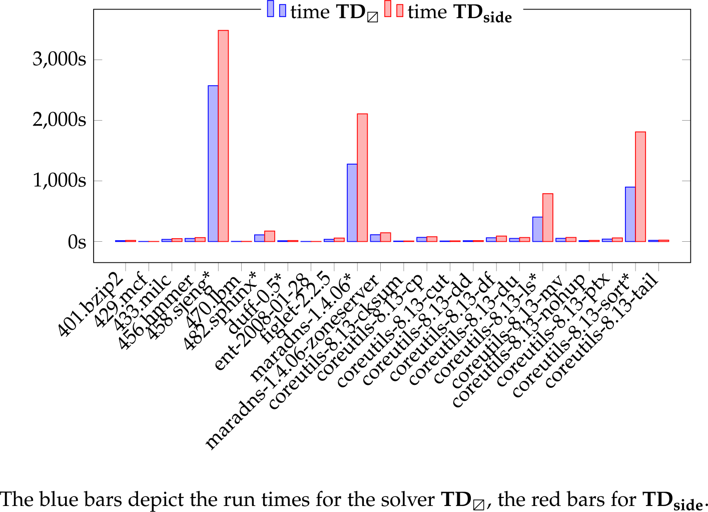
Figure 4. Absolute run times of
 $\textbf{TD}_{\unicode{x29C4}}$
vs.
$\textbf{TD}_{\unicode{x29C4}}$
vs.
 $\mathbf{TD}_{\mathbf{side}}$
.
$\mathbf{TD}_{\mathbf{side}}$
.

Figure 5. Relative run times of
 $\mathbf{TD}_{\mathbf{side}}$
over
$\mathbf{TD}_{\mathbf{side}}$
over
 $\textbf{TD}_{\unicode{x29C4}}$
.
$\textbf{TD}_{\unicode{x29C4}}$
.
Finally, we also compared the impact of reluctantly widening for globals (as in the algorithm from the present paper) with default widening (as considered in Seidl and Vogler Reference Seidl, Vogler and Thiemann2018). The run times of the two variants are the same on average. The detection of widening points for side effects leads to higher precision for globals compared to always widening (which was never more precise). The advantage in precision depends on the configuration of the analyzer as well as the analyzed program. 21 out of the 24 benchmarks had higher precision. Of those, the average increase of precision was 2.94%. The highest precision benefit was 25% for the benchmark 429.mcf.
All in all, we find that the optimization for space consumption had a significant beneficial impact on the practical behavior of the resulting solver – a factor of five in the number of unknowns may be a game changer for the overall space consumption, even at the expense of longer running times. On the given benchmarks, though, it did not result in different (practical) termination behavior.
11. Conclusion
The generic local solver TD from Hermenegildo and Muthukumar (Reference Hermenegildo and Muthukumar1992), Charlier and Van Hentenryck (Reference Charlier and Van Hentenryck1992) is not suited to deal with complicated abstract domains with infinite strictly ascending and/or descending chains. Equipping the original TD with warrowing as in Apinis et al. (Reference Apinis, Seidl, Vojdani, Probst, Hankin and Hansen2016) on the other hand results in a solver which is only guaranteed to terminate for monotonic systems of abstract equations, and as is, provides no support for side-effecting. Therefore, we have provided three enhancements or additions. First, we considered extra program logic to conceptually guarantee termination for arbitrary systems of abstract equations – whenever only finitely many unknowns are encountered. We then showed how the self-monitoring capability of the solver can be used to reduce space consumption by only storing values at unknowns where also widening and narrowing should be applied. We finally indicated how these solvers can be extended to local generic solvers that operate on side-effecting systems of abstract equations. All three solvers could be proven to conceptually terminate (whenever only finitely many unknowns are encountered). The terminating variant could be proven sound by referring to the lower monotonization of the system of abstract equations. In the space-efficient version, that concept had to be complemented with an argument about consistent closures of mappings. In presence of side effects, we additionally had to collect all occurring side effects before-hand and apply the lower monotonization only then.
Compared to the preceding conference version of this paper (Seidl and Vogler Reference Seidl, Vogler and Thiemann2018), we have elaborated the proofs considerably. In particular, we have provided detailed invariants for the solvers to hold, which can be formally verified by local reasoning over the code. We have also generalized the concept of description relations between concrete and abstract unknowns and illustrated the approach by meaningful examples. Finally, we have re-done the experimental evaluation in order to take the latest evolution of the analyzer Goblint into account, which has introduced a variety of improvements, for example, at the treatment of integer domains and conditions, and removed a series of subtle soundness bugs. The goal thereby was to pin-point the impact of design decisions such as using
 $\textbf{TD}_{\unicode{x29C4}}$
vs. the new one, the
$\textbf{TD}_{\unicode{x29C4}}$
vs. the new one, the
 $\mathbf{TD}_{\mathbf{side}}$
vs. TDspaceτ+side or to what extent the novel technique of auto-detection of widening points at side-effected unknowns is preferable to default widening. Practically, the terminating solver with side effects as well as its space-efficient version turned out to be promising fixpoint engines for static analyzers based on side-effecting systems of equations. Further experimentation is required to evaluate how well these solvers behave for advanced static analyses, for example, for complicated relational domains or more sophisticated analyses of dynamic data structures.
$\mathbf{TD}_{\mathbf{side}}$
vs. TDspaceτ+side or to what extent the novel technique of auto-detection of widening points at side-effected unknowns is preferable to default widening. Practically, the terminating solver with side effects as well as its space-efficient version turned out to be promising fixpoint engines for static analyzers based on side-effecting systems of equations. Further experimentation is required to evaluate how well these solvers behave for advanced static analyses, for example, for complicated relational domains or more sophisticated analyses of dynamic data structures.
It also remains for future research to explore in how far information gathered during the fixpoint iteration itself can systematically be used for further increasing either precision or efficiency of TD solvers.
Conflicts of interest
The authors declare none.
Appendix A. The Original Solver TD
For a better comparison, we recall the original solver TD in the formulation of Fecht and Seidl (Reference Fecht and Seidl1999). This version is slightly more generic than the versions presented in Hermenegildo and Muthukumar (Reference Hermenegildo and Muthukumar1992), Charlier and Van Hentenryck (Reference Charlier and Van Hentenryck1992) as it does not refer explicitly to partial tabulation of procedure summaries. In order to deal with non-monotonicity, the presented version performs an accumulating iteration, that is, updates maintained values of unknowns with the least upper bound of the respective old value and the new contribution. Side-effecting is not supported.
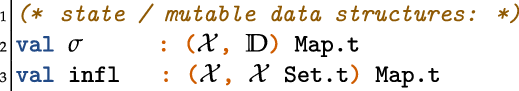
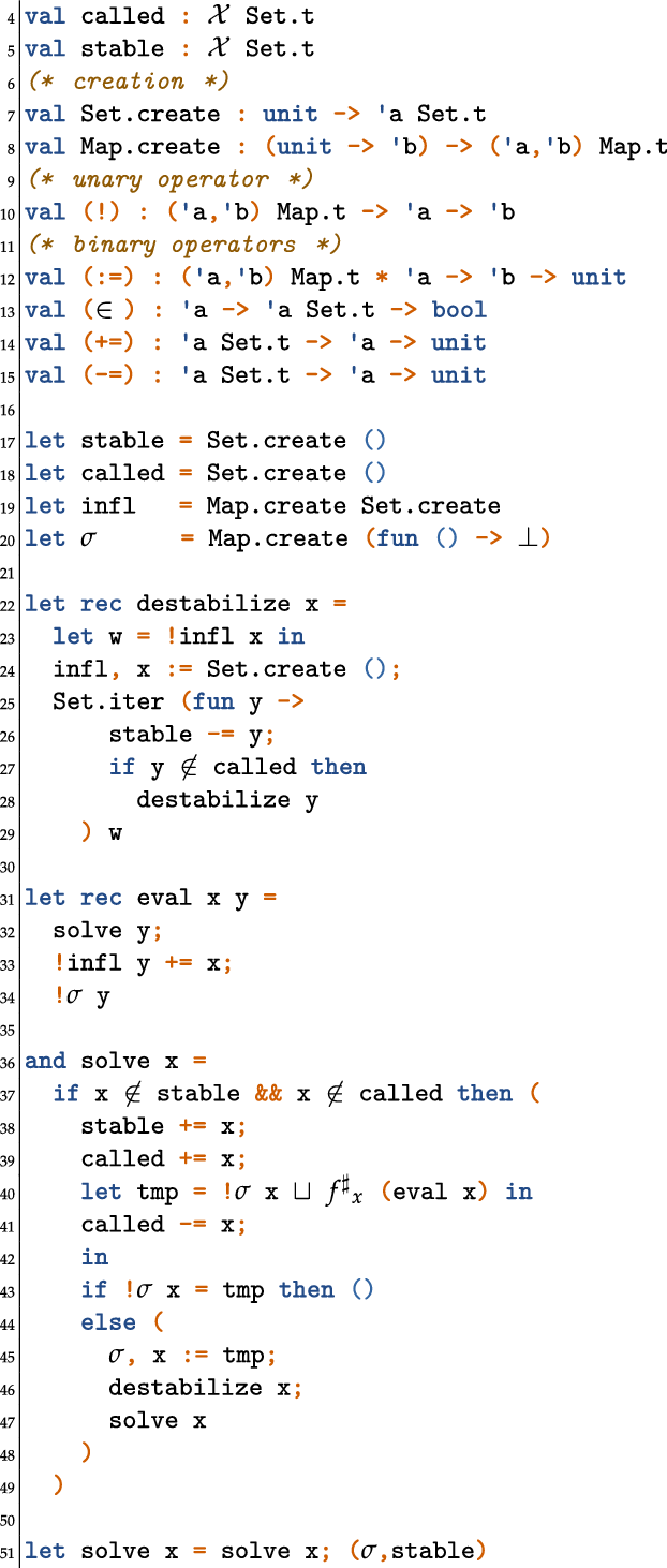
Similar to the solvers
 $\mathbf{TD}_{\mathbf{term}}$
,
$\mathbf{TD}_{\mathbf{term}}$
,
 $\mathbf{TD}_{\mathbf{space}}$
or TDspaceτ+side, the algorithm starts with calling solve for a particular unknown
$\mathbf{TD}_{\mathbf{space}}$
or TDspaceτ+side, the algorithm starts with calling solve for a particular unknown
 $x_0$
. By means of the two functions solve and eval, it descends into unknowns accessed during the evaluation of right-hand sides for recursive evaluation. Similar to what we still do, dependencies between unknowns are detected and recorded on-the-fly. Thereby, the function destabilize for removing unknowns, possibly affected by an update to the value of
$x_0$
. By means of the two functions solve and eval, it descends into unknowns accessed during the evaluation of right-hand sides for recursive evaluation. Similar to what we still do, dependencies between unknowns are detected and recorded on-the-fly. Thereby, the function destabilize for removing unknowns, possibly affected by an update to the value of
 $\sigma$
for an unknown, is identical in our algorithms.
$\sigma$
for an unknown, is identical in our algorithms.
It is mentioned in Charlier and Van Hentenryck (Reference Charlier and Van Hentenryck1992) that an extension of the algorithm with widening is possible. No mechanism, though, is provided for detecting widening points on-the-fly. Also, no intertwined narrowing iteration is introduced. Since no widening/narrowing points are at hand, it seems inevitable to use accumulating updates for all unknowns. Instead, our solvers apply such merging at widening/narrowing points only (and there then together with
 $\nabla$
or
$\nabla$
or
 $\Delta$
) – while at all other points, the old value in
$\Delta$
) – while at all other points, the old value in
 $\sigma$
is replaced (or just recomputed).
$\sigma$
is replaced (or just recomputed).
Appendix B. The Solver TDspace with Caching
The generic local solver TDspaceτ enhances solver
 $\mathbf{TD}_{\mathbf{space}}$
by additionally caching the values for all unknowns
$\mathbf{TD}_{\mathbf{space}}$
by additionally caching the values for all unknowns
 $y\not\in\textit{point}$
which intermediately have been computed during the evaluation of a right-hand side
$y\not\in\textit{point}$
which intermediately have been computed during the evaluation of a right-hand side
 $f^\sharp{}_x$
for some unknown
$f^\sharp{}_x$
for some unknown
 $x\in\textit{point}$
.
$x\in\textit{point}$
.
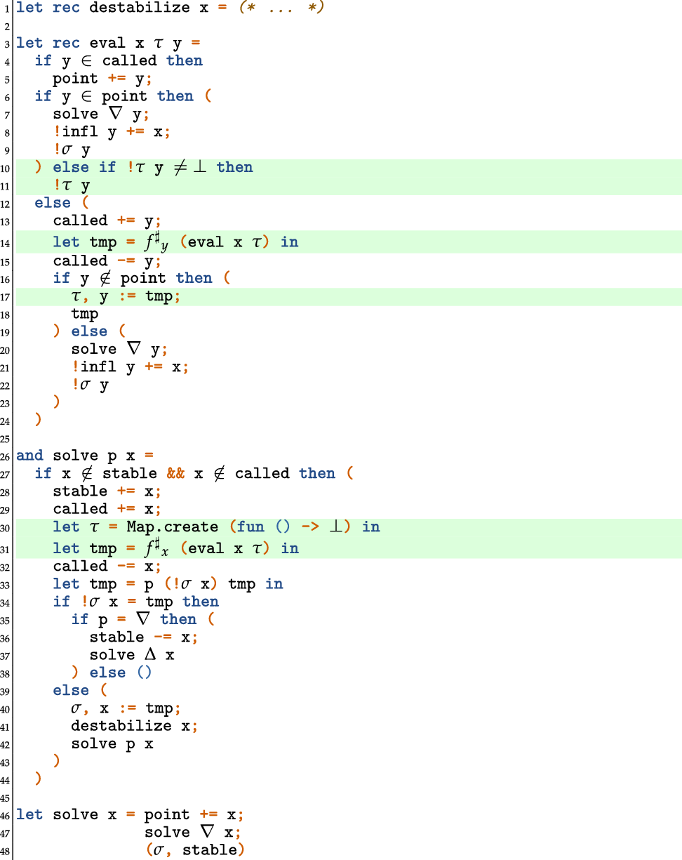
The central modification of solver
 $\mathbf{TD}_{\mathbf{space}}$
is that a fresh mutable map
$\mathbf{TD}_{\mathbf{space}}$
is that a fresh mutable map
 $\tau$
is created before evaluation of the right-hand side
$\tau$
is created before evaluation of the right-hand side
 $f^\sharp{}_x$
inside a call
$f^\sharp{}_x$
inside a call
 $\textsf{solve}\,p\,x$
. That map then is passed to the function
$\textsf{solve}\,p\,x$
. That map then is passed to the function
 $\textsf{eval}$
as an additional argument. In a call
$\textsf{eval}$
as an additional argument. In a call
 $\textsf{eval}\,x\,\tau\,y$
, x is an unknown in
$\textsf{eval}\,x\,\tau\,y$
, x is an unknown in
 $\textit{point}$
whose right-hand side is currently under evaluation;
$\textit{point}$
whose right-hand side is currently under evaluation;
 $\tau$
is the mutable map created in the surrounding call
$\tau$
is the mutable map created in the surrounding call
 $\textsf{solve}\,p\,x$
, and y is the unknown whose value is currently queried. The value of
$\textsf{solve}\,p\,x$
, and y is the unknown whose value is currently queried. The value of
 $\tau\,y$
is only queried when
$\tau\,y$
is only queried when
 $y\not\in\textit{called}\cup\textit{point}$
. When
$y\not\in\textit{called}\cup\textit{point}$
. When
 $\tau\,y$
is found to be different from
$\tau\,y$
is found to be different from
 $\bot$
, this value will be returned. Otherwise, evaluation of
$\bot$
, this value will be returned. Otherwise, evaluation of
 $f^\sharp{}_y\,(\textsf{eval}\,x\,\tau)$
proceeds as in
$f^\sharp{}_y\,(\textsf{eval}\,x\,\tau)$
proceeds as in
 $\mathbf{TD}_{\mathbf{space}}$
. If after evaluation, y still is not contained in
$\mathbf{TD}_{\mathbf{space}}$
. If after evaluation, y still is not contained in
 $\textit{point}$
, the new value for y is recorded in
$\textit{point}$
, the new value for y is recorded in
 $\tau$
and then returned.
$\tau$
and then returned.
Appendix C. The Combined Solver TDspaceτ+side
In this appendix, we finally put all ingredients into one generic solver.
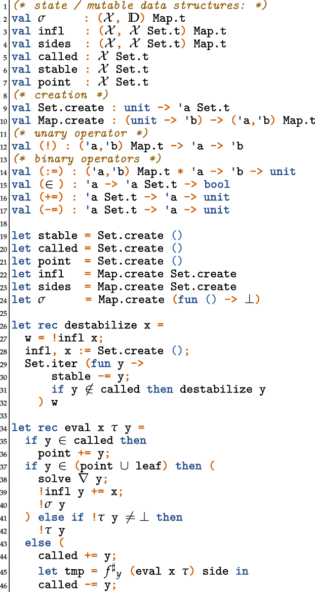
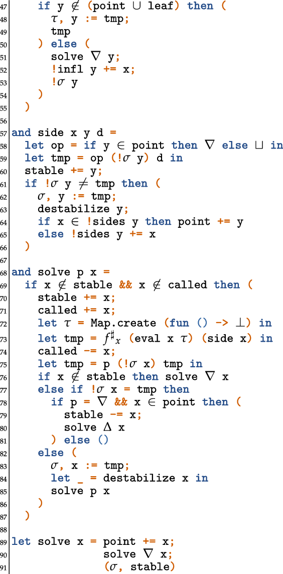
This solver now proceeds essentially as the solver TDspaceτ – but additionally takes side effects into account. This means in particular that unknowns from the set leaf, that is, those which may receive contributions via side effects, must now be treated by the function eval like unknowns from point.


 Open access