

1. The Need for Stochastic Models for Insurers
Modelling has long been a critical component of life insurance companies, and this historically arose due to the complexity and long dated nature of the liabilities.
One can go all the way back to the development of a with-profits product, first suggested by James Dodson in 1756, in a document entitled “First Lectures on Insurance”. A key feature was the development of a whole-of-life assurance policy, when only short-term (1–2 year) assurance was sold. The summary features included a description of a with-profit system “where participating and non-participating policies were simultaneously provided” and “The surplus on non-participating business would be distributed equitably amongst participating policyholders, in proportion to how much profit their own policies had generated for the corporation by virtue of their longevity”. The product as described above was later implemented by Equitable Life, which subsequently led the development of Life Assurance within United Kingdom.
The with-profits product also emerged as a key product within the United Kingdom, and along with it the role of an actuary to calculate and model the distributions from the surplus of the with-profits fund. The sophistication in modelling increased over time as the with-profits product emerged, with huge strides in the understanding of mortality, following the founding of the Institute of Actuaries in 1848 (Faculty of Actuaries in 1856). A detailed exposition of these developments can be found in the 8 volume History of Insurance (Jenkins & Yoneyauma, Reference Jenkins and Yoneyauma2000).
Most of the models at this time still had a single view of the future, either best-estimate or with various shades of prudence for the purposes of pricing, valuation and reserving. This huge volume of actuarial thought developed at a time when the main investments of insurance companies were fixed interest, loans and securities, which provided relatively low yields at a time when long-term inflation was virtually nil (19th century), and focussed very much on deterministic models. The conventional actuarial concept of a single fixed rate of interest was considered reasonably appropriate in these circumstances. However, over the 30 years from 1920 to 1950, British life offices started increasingly investing in equity and property, with the equity allocations increasing from 2% in 1920 to 21% by 1952 (Turnbull, Reference Turnbull2017) which increased the importance and complexity of the asset model.
“Now I am become Death, the destroyer of worlds”.
These were the immortal words that that were brought to Robert Oppenheimer’s mind as he saw the detonation of the first ever atomic bomb in 1945 (Wikipedia, n.d.). 1945 was also the year that the first electronic computer was built at the University of Pennsylvania in Philadelphia by John Mauchly and Presper Eckert. Electronic Numerical Integrator And Computer (ENIAC) was an impressive machine, it had 18,000 vacuum tubes with 500,000 solder joints (Metropolis, Reference Metropolis1987).
ENIAC brought the renaissance of an old mathematical technique known at the time as statistical sampling. Statistical sampling had fallen out of favour because of the length and tediousness of the calculations.
While recovering from an illness in 1946 Stanislaw Ulam questioned the probability of winning a game of Canfield Solitaire (Wikipedia, n.d.). After spending a lot of time trying to come up with an abstract solution to the problem, he hit upon the idea of using sampling methods which could be used with the aid of fast computers (Eckhardt, Reference Eckhardt1987).
During the review of ENIAC in spring of 1946 at Los Alamos, Stanislaw Ulam discussed the idea of using Statistical sampling with John von Neumann to solve the problem of neutron diffusion in fissionable material. This piqued Neumann’s interest and in 1947 he sent a handwritten note to Robert Richtmyer outlining a possible approach to the method for solving the problem as well as a rudimentary algorithm (Neumann & Richtmyer, Reference Neumann and Richtmyer1947). This was most likely the first ever written implementation of the statistical sampling technique.
It was during this time that Nicholas Metropolis suggested the name Monte Carlo Method – a suggestion not unrelated to the fact that Stanislaw Ulam had an uncle who would borrow money from relatives because he “just had to go to Monte Carlo” (Metropolis, Reference Metropolis1987).
Metropolis and Ulam published their seminal paper on the Monte Carlo method in 1949 (Metropolis & Ulam, Reference Metropolis and Ulam1949). The method was implemented successfully for use in development of the Hydrogen Bomb and subsequently went on to be used in a wide array of fields including finance.
One of the core aspects of the Monte Carlo method is the use of Random Numbers to see the evolution of the decision paths. For the first implementation of the Monte Carlo method, the pseudo random number generator used was von Neumann’s “middle-square digits” (Metropolis, Reference Metropolis1987). The generator produced uniform random deviates which were then transformed into non-uniform deviates based on a transformation function.
Like Monte Carlo methods, random number generation has evolved substantially since their use in 1949 and continues to be developed at a rapid pace within the field of mathematical finance as well as outside.
A paper by the Maturity Guarantee Working Party (MGWP) (Benjamin et al., Reference Benjamin, Ford, Gillespie, Hager, Loades, Rowe, Ryan, Smith and Wilkie1980) summarises the need for stochastic models quite eloquently:
“The traditional methods of life office valuation are deterministic with margins incorporated implicitly in the basis. This is the same as using expected values in the commonly understood statistical sense but with a cautious probability distribution. This approach works in practice because, on the one hand, deaths are usually independent and there are large numbers exposed to risk and, on the other hand, the investment risk can be matched. The result is a small variability in claims”.
“In the case of maturity guarantees, however, the investment risk cannot be matched and policies with guarantees maturing at the same time are not independent. There is, therefore, a much greater variability in claims. The Working Party was, therefore, looking for a distribution of claim values and was looking at one tail of that distribution where the proceeds arising from the unit fund were less than the amount guaranteed. If expected values had been used, the initial contingency reserves for maturity guarantees would have been zero when taking into account future premiums for the guarantee”.
Thus, there was an increasing awareness of the uncertainty in future solvency driven by the inherent uncertainty in the capital markets, as indicated in Figure 1.
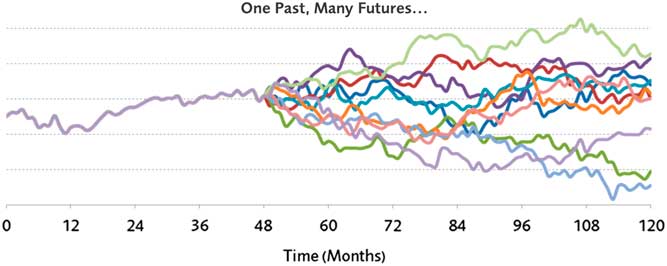
Figure 1 An example simulation of a single path
The need for stochastic models for a life insurer with path-dependent liabilities and a global asset allocation then provides some challenges, which we aim to summarise in the next section.
2. The Challenge Inherent in Stochastic Asset Models (SAMs)
In the context of history, whilst stochastic asset modelling has come relatively late to the party of complex actuarial modelling, it is perhaps the most challenging aspect in some respects. In addition to the pure inherent uncertainty of future capital market outcomes, there are a number of other factors which compound the complexity, as we see in Figure 2.
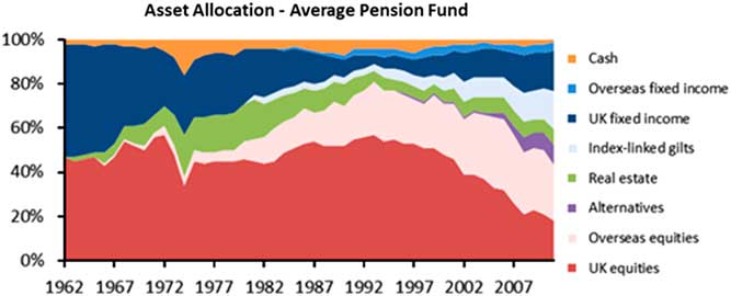
Figure 2 Asset allocation for an average pension fund (United Kingdom)
2.1. The Increasingly Global Nature of the Assets
UK institutional investors have followed a long-term trend of diversifying their portfolios both geographically and from an asset class perspective. While the average UK pension fund was almost wholly invested in domestic equities and domestic bonds in the 1960s, UK assets now occupy a minority share of their portfolio as institutions diversify geographically into overseas markets. Similarly, the portfolios have also been diversified at an asset class level, including real estate and other alternatives. Even within asset classes, diversification is achieved through increasing granularity into sub-asset classes with differing risk and return characteristics.
The changing profile of asset portfolios has improved the overall risk-adjusted returns and insulated portfolios from idiosyncratic risks and political uncertainty specific to the United Kingdom. However, they have added additional layers of complexity to the stochastic modelling of risks and returns for each asset class which determines the overall risk and returns profile of the portfolio.
A truly accurate model of the asset world would potentially be as large as the asset world itself, given the inter-linked nature of all asset classes. Capital can move in three ways, either within different segments of an overall asset class, e.g. a movement from short dated government bonds to long dated government bonds, or from one overall asset class to another, e.g. bonds to equities, or internationally from one country to another. Ideally the SAM under consideration would capture all these features.
2.2. Long Dated Liabilities, Which Require Extrapolation in Time
The other key factor is the long dated nature of the liabilities, which require extrapolation of scenarios across a long period of time. Thus (philosophically) an accurate model not only needs to be as large as the asset world, but run several times faster to extrapolate in time.
This feature was further embedded in the insurance company valuations as part of the Realistic Balance Sheet, introduced by the Prudential Sourcebook, 2003. This made it even clearer that a significant proportion of balance sheet volatility arose from the asset side of the balance sheet.
The issue of duration mismatching has frequently arisen in asset liability modelling, where assets of sufficient duration to match the liabilities have not been available historically, with the issue coming into sharper focus in the historically low interest rate environment of the past 10 years since the 2008 global financial crisis. In response to this, bonds of longer duration have been issued (mainly by governments) with keen take up from insurers, together with investing in long term property lease arrangements which offer the required duration to match the length of long dated liabilities, and hence reduce potential balance sheet volatility.
2.3. Capital Regulations, Which Require Extrapolation in Terms of Probability
The third step in the increasing complexity was the nature of the capital regulations, first introduced in 2004 as part of the Individual Capital Adequacy Standards (ICAS) regime introduced by the Financial Services Authority (FSA), and latterly the Solvency II regime adopted by the European Insurance and Occupational Pensions Authority (EIOPA). This meant that, not only was one required to model the global asset universe, one needed to be able to run the valuation faster than real time in order to be useful. Finally, the Solvency II regulations required the model to extrapolate to extreme probabilistic events that were often far outside an average (or even extreme) career as well as beyond the reasonable histories of a large number of asset classes.
3. Evolution of Asset Models
Having taken as input a large range of literature on Actuarial history, conducted a range of interviews with developers and users of economic scenario generators (ESGs), and pored through a range of Actuarial and Academic papers, journals and books, it appears that there were a number of stages in the evolution of ESGs, as shown in Figure 3.
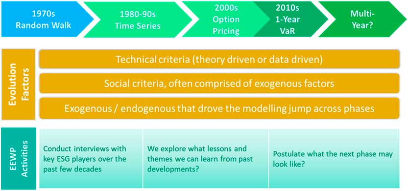
Figure 3 Evolution of economic scenario generators
This led to broadly four stages of ESGs, and we shall explore each in further detail in the next four sections:
■ Random Walk Models
■ Time Series Models
■ Market Consistent (MC) and Arbitrage-Free Models
■ Value at Risk (VaR) Models
Whilst the VaR Models are in practice less complex relative to the other ESGs and there is a strong distinction between the two; in general, ESGs are generally time series models that consider the evolution of an economic quantity over time, whereas VaR models focus more on a statistical distribution of outcomes over a shorter time period – usually up to 1 year in the insurance industry. Nevertheless, we have included them both in the scope of this paper as their history is to some extent interlinked.
4. Random Walk Models
In the warm summer months of 1905, Karl Pearson was perplexed by the problem of the “random walk”, as illustrated in Figure 4. He appealed to the readers of Nature for a solution as the problem was – as it still is – “of considerable interest”. The random walk, also known as the drunkard’s walk, is central to probability theory and still occupies the mathematical mind today. Among Pearson’s respondents was Lord Rayleigh, who had already solved a more general form of this problem in 1880, in the context of sound waves in heterogeneous materials. With the assistance of Lord Rayleigh, Pearson concluded that “the most probable place to find a drunken man who is at all capable of keeping on his feet is somewhere near his starting point!” (Nature, 2006).
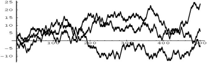
Figure 4 Random Walks
In Reference Bachelier1900 Louis Bachelier published his truly remarkable doctoral thesis, La Théorie de la Spéculation (Theory of Speculation), on random walk or Brownian motion. Bachelier is credited with being the first person to apply the concept of random walk to modelling stock price dynamics and calculating option prices. It was his pioneering research that eventually led to development of the efficient market hypothesis (Rycroft & Bazant, Reference Rycroft and Bazant2005).
It was Norbert Weiner who provided the rigorous mathematical construction of Brownian motion and proceeded to describe many of its properties: it is continuous everywhere but nowhere differentiable. It is self-similar in law, i.e. if one zooms in or zooms out on a Brownian motion, it is still a Brownian motion. It is one of the best known Lévy processes (càdlàg stochastic processes, i.e. right continuous left limit process with stationary independent increments) and it is also a martingale.
It was in 1951 in the Memoirs of the American Mathematical Society; Volume No. 4, a paper titled “On Stochastic Differential Equation” was published by Kiyoshi Ito (Reference Ito1951). This seminal work first introduced the concept of “Ito’s Lemma” which went on to become a fundamental construct in financial mathematics.
Around the same time Harry Markowitz (Reference Markowitz1952) published his paper “Portfolio Selection” which was the first influential work on mathematical finance which captured attention outside academia. Markowitz (Reference Markowitz1952), the paper, together with his book “Portfolio Selection: Efficient Diversification of Investments” (Markowitz, Reference Markowitz1959), laid the groundwork for what is today referred to as MPT, “modern portfolio theory”.
Prior to Markowitz’s work, investors formed portfolios by evaluating the risks and returns of individual stocks. Hence, this leads to construction of portfolios of securities with the same risk and return characteristics. However, Markowitz argued that investors should hold portfolios based on their overall risk-return characteristics by showing how to compute the mean return and variance for a given portfolio. Markowitz introduced the concept of the efficient frontier which is a graphical illustration of the set of portfolios yielding the highest level of expected return at different levels of risk. These concepts also opened the gate for James Tobin’s super-efficient portfolio and the capital market line and William Sharpe’s formalisation of the capital asset pricing model (CAPM) (Rycroft & Bazant, Reference Rycroft and Bazant2005).
This leads to a theoretically optimal asset mix where one can define a utility function, and subsequently choose portfolio weights to maximise expected utility. In practice, utility functions contain unknown risk aversion parameters, so we use theory to explain the relationship between asset mix and risk aversion and identify “efficient” portfolios that are best for a given investor’s risk preferences.
There were several advantages to random walk models; they captured the key moments of risk, return and correlation of different asset classes. They were also practical and intuitive, with a small number of intuitive parameters and easily connected to the efficient markets hypothesis. Additionally, the common collection and reporting of historical statistics made them very amenable to calibrate to historical data.
A further development in financial economics came in 1973, when two papers in two different journals had a major impact on the world of modern finance. This biggest impact to the Actuarial profession was not until much later, as we went on a journey through time series models, and the Wilkie model in particular.
5. Time Series Models
5.1. A brief history of time series models
First, it is appropriate to define a time series as a stretch of values on the same scale indexed by a time-like parameter.
The analysis of time series history stretches back to at least the 10th or 11th century AD, where a graph based on time series speculated on the movements of the planets and sun. In this paper we are interested in time series modelling or forecasting – the next step on from the analysis of a time series.
Contemporary time series analysis began in the late 1920s and 1930s with likes of George Udny Yule and Sir Gilbert Thomas Walker. Moving averages were introduced to remove periodic fluctuations in the time series, e.g. fluctuations due to seasonality, and Herman Wold introduced ARMA (AutoRegressive Moving Average) models for stationary series. A non-mathematical definition of a stationary time series is a time series in which there are no systematic changes in mean (equivalent to no trend), there is no systematic change in variance and no periodic variations exist.
1970 saw the publication of “Time Series Analysis” by G. E. P. Box and G. M. Jenkins (Reference Box and Jenkins1970), containing a full modelling procedure for individual series: specification, estimation, diagnostics and forecasting. Box-Jenkins procedures are perhaps the most commonly used procedures for time series analysis and many techniques used for forecasting and seasonal adjustment can be traced back to the work of Box and Jenkins.
In forecasting, the use of multivariate ARMA and VAR models (Vector Auto Regressive) has become popular. However, these are only applicable for stationary time series and economic time series often exhibit non-stationarity. More precisely, a linear stochastic process whose characteristic equation has a root of 1 (a unit root) is non-stationary. Tests for unit roots were developed during the 1980s. In the multivariate case, it was found that non-stationary time series could have a common unit root. These time series are called cointegrated time series and can be used in so called error-correction models within which both long-term relationships and short-term dynamics are estimated. The use of error-correction models has become invaluable in systems where short-run dynamics are affected by large random disturbances and long-run dynamics are restricted by economic equilibrium relationships.
Another line of development in time series, originating from Box–Jenkins models, are the non-linear generalisations, mainly ARCH (Auto Regressive Conditional Heteroscedasticity) – and GARCH – (G=Generalised) models. These models allow parameterisation and prediction of non-constant variance. These models have thus proved very useful for financial time series.
The 2003 Nobel Memorial Prize in Economic Sciences was shared by C. W. J. Granger and R. F. Engle. Granger discovered cointegrated time series and Engle found that ARCH models capture the properties of many time series and developed methods for the modelling of time-varying volatility.
5.2. Actuarial implementation of time series models
In November 1984 A. D. Wilkie presented to the Faculty of Actuaries his paper “A Stochastic Investment Model for Actuarial Use”. In his introduction to the model, Wilkie describes the advantage of a stochastic model – allowing the user to move beyond considering the average outcome and look at the range of outcomes. In the language of the previous section, the Wilkie model is essentially an ARMA modelFootnote 1 but the relationships between the modelled variables does add some complications.
The model described in the 1984 paper applied many of the ideas of time series modelling and forecasting to produce a SAM. Wilkie had been a member of the 1980 MGWP which developed a reserving model for (unit linked) maturity guarantees. The MGWP modelled only equity prices, but did adopt a time series approach based on historic values of the De Zoete equity index. The MGWP modelled the equity price as the ratio of dividend pay-out and the dividend yield. The dividend pay-out was modelled as a random walk with non-zero mean with the dividend yield fluctuating around a fixed mean. The 1984 paper adopted a similar approach for equities, but extended it to other asset classes by adding inflation and a long-term fixed interest yield.
The 1984 paper adopted a “cascade” structure to link the modelled investment variables, with inflation as the entry point. In the 1970s and early 1980s inflation fluctuations, as shown in Figure 5, had a large influence on asset prices.
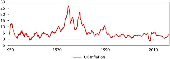
Figure 5 UK inflation from 1950 (Source: ONS)
Professor Wilkie wrote:
“The substantial fluctuations that have been observed in the rate of inflation, the prices of ordinary shares and the rate of interest on fixed interest securities lead one to wish to consider more carefully likely possible future fluctuations in these variables. The actuary should not only be interested in the average return that may be achieved on investments, but in the range of possible returns. Unless he does this, he cannot know to what extent any single figure he chooses is sufficiently much “on the safe side”. A consideration also of the possible fluctuations in investment experience may be of value in considering alternative strategies for investment policy, bonus declaration, etc”.
“The classical model used by financial economists to describe the stochastic movement of ordinary share prices has been that of a random walk. The MGWP showed that, over a long time period, a model based on dividends and dividend yields was more appropriate”.
It is interesting to observe that Professor Wilkie chose a specific time series formulation with two primary and two secondary variables over a fuller multi-variate structure. Wilkie clearly states in the paper that he is considering a model suitable for actuarial use – over the long term – and distinguishes an actuarial model from a model that an economist or statistician might build to prepare short term forecasts.Footnote 2 Wilkie’s specific time series formulation is discussed in a separate note (itself 30 pages long). The formulation reflects the relationships Wilkie found in data from UK time series (1919–1982) and that were considered appropriate for the intended use of the model – with the process adopted being transparent. Whilst the formulation is more parsimonious than a full multi-variate structure, it is far from simple – e.g. the Consol’s yield is a third-order autoregressive process.
The 1984 paper describes the model in full but the cascade structure linking the investment variable is described in Figure 6.
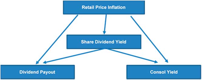
Figure 6 Cascade structure of Wilkie model (Source: Wilkie, Reference Wilkie1984)
Wilkie extended the model presented in the 1984 paper in a 1995 paper. In the period between the two papers the actuarial profession had reviewed the model’s structure (Geoghegan, Reference Geoghegan, Clarkson, Feldman, Green, Kitts, Lavecky, Ross, Smith and Toutounchi1992), with assistance from Wilkie, and the 1995 update (Wilkie, Reference Wilkie1995) addressed some of the challenges and also extended the asset coverage of the model.
5.3. Actuarial use of time series models
The Wilkie model was quickly applied to a range of actuarial issues in insurance, investment and pensions work. It is interesting to speculate on why use of the Wilkie stochastic model became so widespread. Some of the key themes behind the rapid adoption of the Wilkie model identified by the authors of this paper were:
■ Publication and transparency – The Wilkie model was specifically intended for the longer-term problems which concern actuaries. Its design was transparent and had been formally discussed by the Faculty of Actuaries which gave it credibility. There are occasional references in the discussion of actuarial papers to other, proprietary, stochastic models but their closed nature is seen as a disadvantage.Footnote 3 Similarly, there are occasional references in actuarial discussions to investment houses having inspected the Wilkie model and had no significant criticism of it.Footnote 4
■ Practicality – The Wilkie model was relatively easy to apply – it could be coded into a spreadsheet. The published details included all the formulae and recommended parameters. Wilkie (Reference Wilkie1985) subsequently published a paper to the Institute of Actuaries Students’ Society in which he applied the model to a variety of actuarial topics.
■ Consistency with prior beliefs – This theme is contentious and is anecdotal. The structure and calibration of the Wilkie model implied that equities displayed mean reversion over terms of a few years. Accordingly, the use of a static “strategic” asset allocation modestly improves expected return for an acceptable level of risk, by increasing equity allocation or making portfolios more efficient (according to the model). This feature was rapidly identified (Wilkie himself described the feature in his 1985 paper to the Institute of Actuaries Students’ Society) but did not halt the widespread use of the model. Arguably the model was merely encoding support for a “buy on a dip” philosophy.Footnote 5 In a similar fashion the Wilkie model’s assumption of normality in residuals limits the occurrence of extremes in the modelled variables – this might be a desirable feature for certain purposes, e.g. concentrating on the most likely outcomes in the longer term and avoiding distortions from past extreme events. Obviously for other purposes, e.g. capital requirements, such features are not desirable.
■ Social factors – again, this theme is necessarily anecdotal. Under this theme we group a variety of factors that we have labelled “social factors”.
o The desire of actuaries to adopt the latest techniques in their work and move beyond just considering the average outcome. The credibility of the Wilkie model helped here.
o Did the rush to apply the technique of new applications lead to a reduced focus on understanding the influence of model features on the analysis being performed?
o Whilst many alternative formulations and calibrations to Wilkie are possible (indeed Wilkie discussed some in the Reference Wilkie1984 paper) the volume of work and the subsequent levels of explanation required (relative to applying “standard” Wilkie) would be enormous.
For the above reasons, and perhaps many more, the Wilkie SAM became the standard for actuarial work for the remainder of the 1980s and much of the next decade.
5.4. Identification of limitations in the Wilkie time series models
The Wilkie model was fundamentally different to the arbitrage-free concepts being developed within the banking world, and it was ultimately the concept of MC valuation that drove a shift away from the time series approach of the Wilkie model.
The actuarial profession gave the 1984 paper a thorough review with the discussion raising many challenges (Wilkie, Reference Wilkie1984). Various speakers challenged parameter values and even the time series analysis that led to Willkie’s model structure. As described earlier, Wilkie’s Reference Wilkie1985 paper to the Institute of Actuaries Students’ Society described how the use of a static “strategic” asset allocation could modestly improve expected return. This feature of the model was in the public domain although the extent of it in a particular application of the model would vary from case to case.
The equity volatility term structure in the Wilkie model implies shares are a good long-term match for inflation linked liabilities, such as many defined benefit pension scheme liabilities. The period following the publication of the Wilkie model was accompanied by a general rise in pension scheme equity allocations – although, of course, this outcome cannot be traced directly to the use of the Wilkie model and the trend was already established before the Wilkie model was published (see Figure 2).
In 1985 the Government Actuary’s Department introduced a requirement for Life Insurers to carry out prescribed stresses to ensure that there was sufficient prudence built into the calculation of liabilities to reduce the risk of insolvency. The additional reserves required under this approach were referred to as Resilience Reserves and reflected the largest adverse difference in movement of asset values and liability values in each of the adverse stresses, allowing the valuation basis to be modified but only in accordance with other regulatory requirements.
Market movements over subsequent years caused some actuaries to believe that fixed prescribed stresses were not effective in creating a consistent level of additional security and indeed a number of modifications were made to these requirements by the Regulators over time. The Actuarial Profession established a Working Party to consider whether some underlying model could be used to introduce a level of stability of effectiveness of the method by varying the stresses in a prescribed way with market conditions. Initially the Working Party utilised the Wilkie model for its work, but swiftly realised that the extent of mean reversion meant that when markets strayed too far from the observed mean, the additional reserves required by such a model would tend to either significantly increase or reduce, to an extent which appeared excessive.
The size of this effect was influenced heavily by the choice of assumed mean and the Working Party developed an alternative approach which was based on the Wilkie model, but under which the mean of the various parameters could be allowed to change, or jump, from one level to another from time to time. This produced interesting results, particularly when applied to historic data. However, around the same time, there was the emergence of a significant shift away from Net Premium valuations on which the Resilience Methodologies at the time were largely based to MC valuations, and policyholder security started to be considered largely in terms of 1-year VaR Capital requirements, so the work was not pursued and never formally published.
Given the wide ranging use of the Wilkie model within the profession it is possible that individual actuaries and companies may well have similarly developed the model along lines specific to their own needs but again without the results being published.
In the discussion of the 1989 paper “Reflections on Resilience” (Purchase et al., Reference Purchase, Fine, Headdon, Hewitson, Johnson, Lumsden, Maple, O’Keeffe, Pook and Robinson1989), Sidney Benjamin stated:
“Professor Wilkie’s model is being used time and time again in actuarial literature. As far as I know it has never been validated. People are just taking it for granted because it is the only one around. I suggest that if we are going to carry on using that model in actuarial literature, we need a Working Party to examine its validity”.
The 1989 resilience paper contains an examination of the Resilience Reserve where the investment returns behave according to the Wilkie model. Benjamin suggests a good starting point for such a validation review would be the 1988 paper from Arno Kitts, “Applications of Stochastic Financial Models: A Review” (Kitts, Reference Kitts1988) prepared whilst a Research Fellow at the University of Southampton. The Working Party that Benjamin had suggested was formed later in 1989 and produced a report in 1992, “Report on the Wilkie Stochastic Investment Model” (Geoghegan, Reference Geoghegan, Clarkson, Feldman, Green, Kitts, Lavecky, Ross, Smith and Toutounchi1992). The Working Party engaged Professor Andrew Harvey of the London School of Economics for review of the statistical procedures behind the model and Professor Wilkie assisted in the review. The report focusses on the statistical quality of the model – particularly to inflation (as it is the entry point for the “cascade”). Alternative model structures are described at a high level but the Working Party make clear their work should be the springboard for further work. The report does contain an interesting discussion on whether the parameters in the model remain constant over time. Professor Harvey pointed out that if actuaries were to make serious use of stochastic models, and to use them in an intelligent and critical way, it is necessary for those in the profession to understand the way such models are built, and the nature of their strengths and weaknesses. This would have implications for the education of actuaries. The discussion, when the paper was presented to the Institute, contains many, and varied views, but the final words here from the Working Party are taken from the report’s Conclusion:
“Further in this respect, several members of the Working Party expressed concerns that practitioners (both actuaries and non-actuaries) without the appropriate knowledge and understanding of econometric and time series models might enthrone a single particular model, and scenarios generated by it, with a degree of spurious accuracy”.
While Wilkie’s model stands out for its impact within the published literature, the 1990s was a time of rapid technical innovation and a number of other models were in use, particularly for pensions work.
The use of stochastic modelling for pensions asset-liability studies was largely carried out within consulting firms, on behalf either of the plan trustees or the sponsoring employer (or, sometimes, both). Several firms sought to establish their credentials in this area by publishing SAMs, although generally more briefly than Wilkie’s paper and without the extensive supporting analysis. Here we summarise some relevant papers.
In the paper “Asset/Liability modelling for pension funds” (Kemp, Reference Kemp1996), Malcolm Kemp proposes using random walk models for real returns, as alternatives to the Wilkie model. Chapman et al. (Reference Chapman, Gordon and Speed2001) described a further updating of this model.
In 1999, Yakoubov et al. (Reference Yakoubov, Teeger and Duval1999) presented their “TY” model to the Staple Inn Actuarial Society. This is a time series model, with many similarities to the Wilkie model.
Dyson & Exley (Reference Dyson and Exley1995) published one of the first models to include a full term structure of interest rates in 1995, in an appendix to their Institute Sessional Paper: Pension Fund Asset Valuation and Investment.
The Institute of Actuaries’ annual investment conferences carried further papers describing stochastic models, including McKelvey’s (Reference McKelvey1996) Canonical Variate Analysis approach, Smith (Reference Smith1997) multi-asset fat-tailed model and Hibbert et al. (Reference Hibbert, Mowbray and Turnbull2001) model. Like Dyson & Exley’s model, Smith’s model and the Hibbert & Turnbull’s model provided a full interest rate term structure in continuous time, now with the added property that the model is arbitrage-free.
These models were published not only with formulae, but also with parameters. Other firms developed proprietary models whose details were published only in part. One example was the paper “Generating Scenarios for The Towers Perrin Investment System”, by John Mulvey (Reference Mulvey1996), published in Towers Perrin’s own journal, Interfaces, in 1996.
Meanwhile, Wilkie continued to enhance his own model by adding further asset classes and other outputs. David Wilkie and Patrick Lee presented a summary paper – A Comparison of SAMs – to the 2000 AFIR conference in Tromso (Lee & Wilkie, Reference Lee and Wilkie2000). As well as comparing some existing models, they further developed Wilkie’s model, providing work-arounds for various earlier model limitations, including extensions to monthly time steps, full yield curve term structures, and some proposals on allowing for parameter estimation error.
6. MC and Arbitrage-Free Models
It was in 1973 that two papers in two different journals had the biggest impact on the world of modern finance. Fischer Black and Myron Scholes (Reference Black and Scholes1973) published the paper “The Pricing of Options and Corporate Liabilities” in the Journal of Political Economy and Robert Merton (Reference Merton1973) published the paper “On the pricing of corporate debt: the risk structure of interest rates” in the in Journal of Finance. These papers introduced methodologies for valuation of financial instruments, in particular one of the most famous equations in finance, the “Black-Scholes” Partial Differential Equation (PDE)
 $${{\partial V} \over {\partial t}}{\plus}{1 \over 2}\sigma ^{2} S^{2} {{\partial ^{2} V} \over {\partial S^{2} }}{\plus}rS{{\partial V} \over {\partial S}}{\minus}rV{\equals}0$$
where $V$
is the option value,
$V$
is the option value, $S$
the underlying asset,
$S$
the underlying asset, $\sigma $
the volatility and
$\sigma $
the volatility and $r$
the risk-free interest rate.
$r$
the risk-free interest rate.
It was during the 1970s that another breakthrough on the industry side was the foundation of the Chicago Board Options Exchange (CBOE). CBOE became the first marketplace for trading listed options. The market was quick to adopt these models and by 1975, almost all traders were valuing and hedging option portfolios using the Black–Scholes model built in their hand calculators. From a tiny market trading only 16 option contracts in 1973, the derivatives market has grown enormously in notional amount to trillions of dollars (Akyıldırım & Soner, Reference Akyıldırım and Soner2014).
The work of Black and Scholes led to an explosion in research in mathematical finance. To recount all the discoveries since 1973 in the world of mathematical finance would be an attempt in futility. Initially simple models (1 factor) but more sophisticated models followed (better able to capture initial yield curve and an implied volatility surface)
■ Examples for interest rates include: Vasicek, Hull White, Cox–Ingersoll–Ross, LIBOR market model.
■ Examples for equities include Geometric Brownian Motion, Geometric Brownian Motion with drift, and extensions to include term structure, volatility surface (see Figure 7), stochastic volatility as well as jumps.
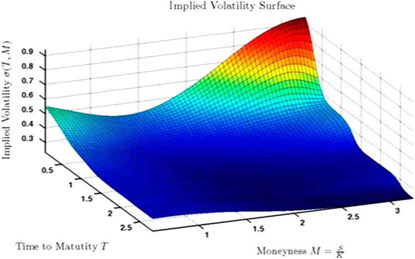
Figure 7 Example of a volatility surface
The work of Black and Scholes was picked up by Academic actuaries relatively quickly, with one of the early papers by Brennan & Schwartz (Reference Brennan and Schwartz1976) from the University of British Columbia in Vancouver, dated December 1975.
However, there was a significant lag before widespread use within the actuarial community specifically within the United Kingdom, partly due to the then alien concept of no-arbitrage and dynamic hedging concepts, and partly because a probabilistic model solving for a specific ruin probability as suggested by Wilkie at least solved the stochastic nature of the issue (see previous chapter), together with the report by the (unit linked) maturity guarantee working party and the subsequent widespread use and adoption of the Wilkie model.
Having said that, it was actually a paper by Professor Wilkie in 1987 on “An Option Pricing Approach to Bonus Policy” (Wilkie, Reference Wilkie1987), that drew the link between option pricing and with profit policies and introduced the idea of option pricing and financial economics to a number of UK Actuaries.
Into the early and mid-1990s, there was increasing awareness and subsequent references to, and discussion about, Financial Economics. For example, in March 1993, there was a Sessional meeting and debate on “This house believes that the contribution of actuaries to investment could be enhanced by the work of financial economics”. This was one of a series of debates on the subject in the mid-90s, both at the Institute and Faculty of Actuaries. The topic of financial economics was also formally noted in a wide ranging paper on “The Future of the Profession”, commissioned by the Councils of both the Institute and Faculty of Actuaries in December 1994. The study was presented by Nowell et al. to the Faculty of Actuaries in November 1995 and the Institute of Actuaries in January 1996 (Nowell, 1996).
In particular, it highlighted a requirement for additional skills to achieve “a better understanding of investment vehicles and financial economics”. The paper also highlighted a need for structurally incorporating the new skillsets in terms of education and Continuous Profession Development (CPD):
■ financial economics;
■ understanding of investment instruments;
■ financial condition reporting (e.g. risk of ruin);
■ a broad-based understanding of risk and finance; and
■ the ability to apply these, together with the more traditional skills, to a wide variety of problems in an innovative way.
On a more practical scale, there was a detailed paper by A. D. Smith (March, Reference Smith1996) on “How Actuaries can use Financial Economics”. The aim of the paper is neatly summarised in the introductory section:
“It is not the purpose of this paper to review established models such the CAPM or the Black-Scholes formula. Instead, I will examine some underlying techniques which have been fruitful in financial economics. Economists have applied these techniques to classical economic problems in order to derive the established models. In this paper I have applied the same techniques to some current actuarial problems, and obtained solutions which fuse traditional actuarial methods with powerful insights from economics”.
The paper goes on to provide a series of case studies, on the concepts of risk neutrality, risk discount rates, arbitrage and their applications to option pricing and asset-liability models and methodology. The first concluding remark was also quite insightful into the novelty of financial economics at the time:
“Actuaries pre-date financial economics by at least a century, but the problems addressed by the two schools intersect to a large degree. Financial economics has opened a Pandora’s box of new concepts and techniques. Many of these techniques were developed in the context of asset selection models. For actuaries, the insight which can be obtained into the behaviour of liabilities and their interaction with assets is at least as important as the asset models themselves. Financial economics is eminently applicable in the traditional areas of actuarial endeavour, namely: insurance, pensions and investments”.
There were also a number of other papers on even more specific applications of financial theory, and one that particularly comes to mind was by Exley et al. (Reference Exley, Metha and Smith1997) on the financial theory of defined benefit pension schemes, presented to the Institute of Actuaries in April 1997.
This focussed on the application of MC valuation techniques to the valuations of pensions schemes, and had a profound impact on the subsequent management and investment strategy of pension schemes.
Meanwhile, there were also some regulatory developments that further enshrined the concept of a MC valuation for an insurer’s balance sheet.
■ 1997 – the International Accounting Standards Board started working on a new accounting standard for insurance.
■ 1999 – The Faculty and Institute Life Board established a working party – the “Fair Value Working Party”. This presented a paper to the Institute and Faculty in November 2001.
■ 2002, 2003 – Consultations published by UK’s FSA.
■ 2003 – FSA published the Integrated Prudential Sourcebook, requiring a MC valuation for any firm with more the £500m in with profit liabilities.
■ This would be soon followed by the Individual Capital Assessment (ICA), which required stressing the newly created MC balance sheet to 99.5th percentile 1-year VaR, which is described more fully in the following chapter.
6.1. Key challenges of MC and Arbitrage-Free Models
These models assume that markets follow the expectations hypothesis, whereby the implied pricing in the market is the best estimate of future outcomes:
■ By construction, the no-arbitrage principal does not follow the CAPM, although the model can be extended by the use of “risk premia” to form a real-world model.
■ More exotic models (e.g. stochastic volatility, jumps) require a greater number of parameters and as such are much more difficult to calibrate, requiring significantly more judgment and (usually) historical data, and being less robust to changes in empirical data.
7. VaR Models
In the early years of the millennium, following a notable regulatory failure, there was a desire to improve the approach to regulatory supervision of UK Life Insurers and particularly with profits companies. Given that one of the key issues was a desire to monitor guarantees and options which existed within life insurance contracts, the use of a MC valuation of liabilities and assets, which was being considered as an accounting standard, formed a natural starting point. However, the previous regulatory framework, which presumed the existence of implicit liability margins, would not sit well with a margin-free MC view of liabilities. Hence a new approach was needed.
Given that banks had developed “ ${\rm VaR}$
” as a mechanism for determining capital adequacy that could be applied to realistic valuations, this appeared a reasonable starting point for insurers. However, the nature of banking and insurance and consequently their supervisory regimes are significantly different so consideration had to be given to the implications of these differences.
${\rm VaR}$
” as a mechanism for determining capital adequacy that could be applied to realistic valuations, this appeared a reasonable starting point for insurers. However, the nature of banking and insurance and consequently their supervisory regimes are significantly different so consideration had to be given to the implications of these differences.
In its simplest form ${\rm VaR}$
requires the identification of the amount of capital required to ensure that in the event of a stress of defined probability the stressed assets held remain sufficient to cover the stressed liabilities. If there is only one risk factor then this concept is relatively simple to model once the distribution of out-turns of the risk are known. However, for even a simple Life Insurer there would usually be multiple risks relating to liability risks, asset risks and valuation basis stresses. For a multi-line Life Insurer, the numbers of risks can be numbered in hundreds. Many of these risks will not be independent and it is normal practice to make allowance for the correlations, typically using copulas. In these cases, there will be a surface of possible combinations of stresses each of which may be considered possible with the defined probability level. The particular stress of this level which produces the largest capital stress is sometimes referred to as the critical stress and is the stress which defines the required capital.
${\rm VaR}$
requires the identification of the amount of capital required to ensure that in the event of a stress of defined probability the stressed assets held remain sufficient to cover the stressed liabilities. If there is only one risk factor then this concept is relatively simple to model once the distribution of out-turns of the risk are known. However, for even a simple Life Insurer there would usually be multiple risks relating to liability risks, asset risks and valuation basis stresses. For a multi-line Life Insurer, the numbers of risks can be numbered in hundreds. Many of these risks will not be independent and it is normal practice to make allowance for the correlations, typically using copulas. In these cases, there will be a surface of possible combinations of stresses each of which may be considered possible with the defined probability level. The particular stress of this level which produces the largest capital stress is sometimes referred to as the critical stress and is the stress which defines the required capital. ${\rm VaR}$
modelling was a requirement of the ICA regime introduced in the UK ~ 2004. A similar requirement is now required under Solvency II. In both cases the defined probability level is a year on year stress with probability of
${\rm VaR}$
modelling was a requirement of the ICA regime introduced in the UK ~ 2004. A similar requirement is now required under Solvency II. In both cases the defined probability level is a year on year stress with probability of $0.5\,\%\,$
. This is sometimes referred to as a 1 in 200 years event.
$0.5\,\%\,$
. This is sometimes referred to as a 1 in 200 years event.
The methodology used here is effectively an extension of the MC methodologies except that the result is typically far more sensitive to the tail of the distribution rather than being averaged over the whole distribution. Also, it is common practice to derive the probability distribution from historic data rather than option prices. In theory the model could be calibrated from option prices but at the levels of risks considered many of the prices used would be far out of the money or deeply in the money and therefore the level of trading would be such that the markets would be far from considered “deep and liquid”. Also markets tend to be preoccupied with specific current threats, which may typically be considered as more likely than required for this form of calibration rather than a long term view of the possible yet extreme events.
One particular feature of this form of modelling which is shared with the MC models, but in this case is far more significant is that the use of correlations applied to a large number of single stresses means there tends not to be a coherent view of the scenarios to which the stressed events correspond and therefore it is difficult to apply expert economic judgement to the plausibility of the model. Further available data for many of the risks involved may be limited, or considered limited, by the lack of relevance of early data. This means that the observed stress events will be limited exaggerated versions of what has actually happened in that period, which may lead to excessive stresses but reduced exposure to those events which have not happened. Consider, e.g. a calibration of interest rate stresses from 10 years of data taken from a period of consistently falling interest rates. One may expect this to overstate the risk of further fall and understate the risk of sharp rises.
Deriving correlations from historic data can also be subject to similar data issues but these can be magnified if it is considered that in stress correlations would be different to those experienced in non-stressed circumstances.
A number of practical and theoretical issues arise with these models, many of which are more significant because of the paucity of data issue referred to above. Fitting a probability distribution to data which does not truly derive from a known distribution potentially leads to high levels of models as indicated by the very different distributions that are derived by trying to fit historic data to a variety of plausible statistical distributions. For example, the Extreme Events working party published a numbers of papers on this topic from 2007–2013 Frankland et al. (Reference Frankland, Holtham, Jakhria, Kingdom, Lockwood, Smith and Varnell2011, Reference Frankland, Smith, Wilkins, Varnell, Holtham, Biffis, Eshun and Dullaway2009, Reference Frankland, Eshun, Hewitt, Jakhria, Jarvis, Rowe, Smith, Sharp, Sharpe and Wilkins2013) and continues to research in the area.
A notable criticism of ${\rm VaR}$
models has been the failure to reflect contagion events, as experienced in the 2008 global financial crisis, when sound financial assets are sold to raise cash in order to meet solvency requirements where other assets have collapsed in value.
${\rm VaR}$
models has been the failure to reflect contagion events, as experienced in the 2008 global financial crisis, when sound financial assets are sold to raise cash in order to meet solvency requirements where other assets have collapsed in value. ${\rm VaR}$
models are typically flat with respect to time, implicitly assuming a constant distribution of asset volatility over time. Other questions that remain open is how one reconciles the implied MC distribution with extreme 1-year VaR stresses derived from historical experience, as well as acknowledgement of the reality that most standard commercial risk packages, by definition, consider VaR on an ex-post basis.
${\rm VaR}$
models are typically flat with respect to time, implicitly assuming a constant distribution of asset volatility over time. Other questions that remain open is how one reconciles the implied MC distribution with extreme 1-year VaR stresses derived from historical experience, as well as acknowledgement of the reality that most standard commercial risk packages, by definition, consider VaR on an ex-post basis.
8. Summary of Past and Current uses of ESGs
The historical and present uses for which an ESG is commonly needed, based on interviews with experienced industry practitioners, are as follows:
■ Strategic Asset allocation.
■ General long-term investment strategy; assessment of investment strategies against investor required return and appetite for risk.
■ Business decisions and management actions based on solvency in future scenarios/probabilities of ruin from an ALM.
■ Product design, prior to launching products.
■ MC Pricing of products once the products have been designed.
■ Financial planning for individuals and institutions.
■ Risk Management and hedging, to control the volatility of the balance sheet.
■ Economic Capital requirements: determining the quantity of assets to ensure liabilities are met with a sufficiently high probability to meet the company’s risk appetite.
■ Regulatory Capital requirements: determining the quantity of assets to ensure liabilities are met with a sufficiently high probability for regulatory solvency.
■ Valuation of complex liabilities or assets, particularly when these contain embedded options or guarantees.
Of the different uses, the last two have largely arisen owing to changes in regulation over the last decade and a half; starting with the Prudential Sourcebook for Insurers (Financial Conduct Authority, 2003), which required every insurance company with more than £500m of with-profit liabilities to use stochastic valuation techniques, and reinforced by Pillar II ICA and its successor Solvency II, which requires a VaR calculation.
Amongst the interviewees, it was widely felt that knowledge of ESGs is important for making decisions thereupon. Given the preponderance of interviews with ESG developers, it is not surprising that the interviewees felt this was an important point. The user must have enough knowledge to understand the limitations of a model and to make sure it is appropriate for the task in hand. This is a lower degree of understanding than a full understanding of the mathematical properties or being able to recreate the model from scratch.
Model calibration (as well as model design) and the challenge that model developers face in communicating the limitations of a model were felt to be important factors in ensuring successful use of an ESG. A number of interviewees pointed to over reliance on model calibrations, whilst not pointing to any specific instances of this occurring in practice. Communication of the data underlying calibrations as well as calibration goals and limitations were additional themes mentioned in the interviews.
There was unanimous agreement that general awareness of ESGs, both amongst users and management, has improved over time. Additionally, there was a general feeling that ESGs should be published in peer reviewed journals. ESG developers interviewed however highlighted that the implementation was important and the low-level implementation of a particular academic model could make a difference to its behaviour and yet the model could still be described as the XYZ academic (and peer reviewed) model. One interviewee commented that the use of non-peer review models placed more responsibility on the model user.
9. Factors Influencing the Evolution of ESGs
The evolution of ESGs occurred over quite a long time period, circa the past 40–50 years, and the evolution can be attributed to a number of factors:
Technical Criteria
■ Goodness of fit to historical data.
■ Ability to forecast outside the sample used for calibration, also called “back-testing”.
■ Desirable statistical properties of estimated parameters, such as unbiasedness, consistency and efficiency.
■ Accuracy in replicating the observed prices of traded financial instruments such as other options and derivatives.
Technical Criteria are frequently listed in Published Papers.
Social Criteria
■ Ease of design, coding and parameter estimation.
■ Commercial timescale and budget constraints.
■ Auditable model output that can be justified to non-specialists in intuitive terms.
■ Compatibility of model output and input data fields with available inputs, and with requirements of model users.
■ Ability to control model output.
■ Meeting regulatory approval e.g. use of ESG in Internal Model Approval Process.
The existence of Social Criteria, such as the above, is inevitable. The existence of Social Criteria is less widely recognised (than the existence of Technical Criteria) and is very rarely discussed in Published Papers.
Technology criteria:
■ Developments in computing power.
■ Use of Monte Carlo methods, and simulation.
■ Black Scholes and option pricing theory.
Regulatory criteria/insurance industry-wide events:
■ Equitable Life.
■ Realistic Balance Sheet (and moving away from statutory Pillar 1 Peak 1 reporting).
■ ICA and Pillar II.
■ Solvency II for European wide adaptation of the above.
Most interviewees have suggested regulatory led changes were the largest factor driving ESG evolution historically, e.g. the move to MC valuations led in the United Kingdom by the FSA. Some changes have been driven by unforeseen changes in the economic environment, e.g. negative interest rates arising out of the 2008 global financial crisis, some user-led by shortcomings in ESGs and some have been developer-led, e.g. the Wilkie model introducing stochastic modelling for the reserving of guarantees.
In general ESG developers wished to improve their models themselves on finding shortcomings. This has been driven partly by a desire to lead the market and by extra research and knowledge that has become available over time. User and regulator dissatisfaction has been less of a driver. Designer dissatisfaction at elements in their ESGs has been very specific to the particular ESG in question.
Historically users found the most pertinent limitations of ESGs to be: a lack of flexibility in models; inability to model some of the real-world behaviour observed, e.g. jumps in equities, negative interest rates; and a lack of calibration to observed market behaviour. Most of the issues have been addressed over time, mainly through a combination of enhanced knowledge and available technology.
The rest of this section discusses the observations that were made by interviewees on the historic development of ESGs from random walk models, followed by time series models, then MC and arbitrage-free models and most recently the 1-year ${\rm VaR}$
models in use for economic capital and related purposes at the present time.
${\rm VaR}$
models in use for economic capital and related purposes at the present time.
There was a broad consensus that time series models (such as the Wilkie model) supplanted random walk models owing to more accurate behaviour relative to the real-world and time series modelling was more realistic and useful to actuaries controlling for actuarial risk. Additionally, there were concerns over the lack of mean reversion in random walk models although a number of interviewees mentioned that the Wilkie model exhibited too strong mean reversion properties. However, since the development of time series models, each new type of ESG has not generally replaced the previous type. Time series, market-consistent and 1y ${\rm VaR}$
models are all still in use but for their own particular purposes.
${\rm VaR}$
models are all still in use but for their own particular purposes.
There was a widespread view amongst the interviewees that MC ESGs were being developed in the late 1990s before realistic balance sheet reporting was introduced in 2003, whilst acknowledging that the FSA changes led to demand for MC-based ESGs. The general consensus at the time was a wariness of the new technique and a focus on perceived inconsistencies within MC valuation techniques, but has come to be seen in a more positive light over time with more objective values and the focus on path dependent modelling.
MC models of the early 2000s were designed for different purposes and required an arbitrage-free framework for all assets which reproduces market pricing to address valuation requirements. The time series model never had this in mind as it is a framework to extend time series modelling of asset prices in the real world. Hence, they were addressing a different problem so cannot be strictly compared. It should be noted however that, whilst the spotlight and focus both in insurance companies and external literature has been on MC models, the Real-World models have continued to co-exist alongside in the background.
The development of ${\rm VaR}$
stimulated another phase of ESG development, although they co-existed with MC models, but used for capital calculations rather than replacing MC ESGs. Presently, the insurance industry has standardised around the 1-year
${\rm VaR}$
stimulated another phase of ESG development, although they co-existed with MC models, but used for capital calculations rather than replacing MC ESGs. Presently, the insurance industry has standardised around the 1-year ${\rm VaR}$
technique, e.g. the 1 in 200 probability of ruin approach under Solvency II. This regulation-led development has put the focus on 1-year
${\rm VaR}$
technique, e.g. the 1 in 200 probability of ruin approach under Solvency II. This regulation-led development has put the focus on 1-year ${\rm VaR}$
techniques rather than multi-year
${\rm VaR}$
techniques rather than multi-year ${\rm VaR}$
models. The interviewees widely expressed the view that there is no point in doing anything more than absolutely necessary in order to gain regulatory approval, further enshrining the 1-year
${\rm VaR}$
models. The interviewees widely expressed the view that there is no point in doing anything more than absolutely necessary in order to gain regulatory approval, further enshrining the 1-year ${\rm VaR}$
current approach. Interviewees suggested multi-period
${\rm VaR}$
current approach. Interviewees suggested multi-period ${\rm VaR}$
models are difficult to run and interpret, and any insight into the long term is missed as a result.
${\rm VaR}$
models are difficult to run and interpret, and any insight into the long term is missed as a result.
Figure 8 shows the perceived balance between empirical data-driven models and Economic Theory-driven models historically over time.
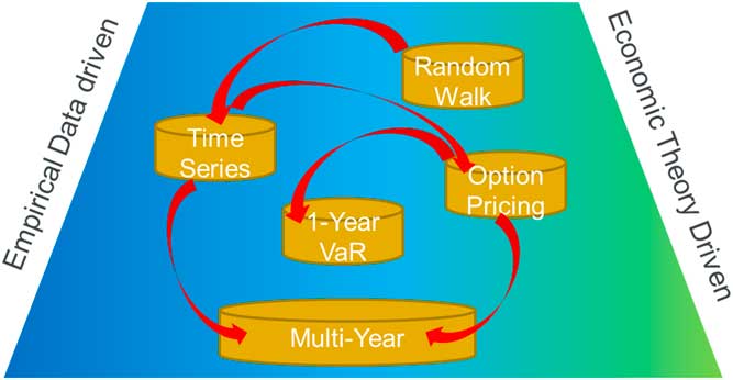
Figure 8 Balance between Empirical data-driven models and Economic Theory. VaR=Value at Risk
10. The Way Forward
This section has been updated for some comments from the wider community at the sessional meeting at Staple Inn on 22 February 2018.
We have some salient observations from the research, discussions and interviews that we have collated over the course of this exercise. Whilst the forces driving change and development of ESGs have changed over time, the need to understand the capital markets and their interactions for investment strategy and business decision making have continued to play a key role. This was the case for the random walk and time series (Wilkie) models. For some years thereafter, the developmental effort was driven by regulations and was focused on more specific applications of MC valuation and 1-year VaR distribution for the ICAS and Solvency II regimes.
This begs the question, what will determine future model developments? There we believe that whilst a natural curiosity and desire to better understand and model the capital markets will lead to a level of steadily increasing sophistication, there may be exogenous factors that lead the development efforts. These could likely include
■ Insurance Regulations – Once again insurance regulations are likely to play a key role in the medium term, this time with the multi-year approach required by the Own Risk and Solvency Assessment (ORSA). This is likely to lead to a renewed focus on longer-term real-world modelling within the insurance industry. For companies that previously relied on external providers, a renewed interest and enthusiasm in the use of in-house capital market views for business and strategy decision making. This will also create a demand in insurance companies for the specialist expertise required for capital markets research and modelling, at the same time as the MiFID II regulations and transparency on commission result in an excess supply from the sell-side (asset management and investment bank research). This may result in an influx of capital markets modelling ideas from the asset management industry.
■ Greater Transparency to customer: Impact of other wider regulations requiring transparency to the customer on the distribution and profile of portfolio outcomes. This was also extensively discussed at the sessional meeting and in particular the need to use capital markets and portfolio modelling for both individuals and institutions.
■ Financial planning and education: At a higher level, it may also require greater awareness of capital markets and financial planning in the actuarial education system, with a particular focus on lifetime and retirement financial planning.
Most of these changes are likely to provide an opportunity to re-define models for the better, whilst some changes such as the ORSA may focus development on a specific aspect for a period of time.
There are other changes which are more difficult to foresee, e.g. the allowance for the evolution of monetary policy, given we have only had a decade of data under the “unconventional” Quantitative Easing programmes deployed by central banks globally, and zero year under any Quantitative Tightening Scenarios. Together with other longer-term trends in capital markets, such as the globalisation of inflation, this would likely lead to a very different starting point for creating an ESG. This was nicely articulated by Stuart Jarvis at the Staple Inn sessional meeting, where he explained that if he were to build the Wilkie model today, he would be using gross domestic product (GDP) growth rather than inflation as the key variable for a causal capital markets model (CMM).
For completeness, it is also worth mentioning technology. At a basic level, the improvement in cloud computing and big data allowing greater granularity of modelling (although to be a good model, the complexity would still need to be traded off against parsimony based on the Occam’s razor principle). At a philosophical level, there may be a disruptive threat in the form of a machine learning algorithm creating a better brute-force ESG. The only saving grace for budding investment professionals is that machine learning algorithms are constrained by Father Time, in that they can only learn as fast as the markets operate in real time (which is still much faster than any human …)
We should also consider learnings from different countries where the use of ESGs has been very different from the United Kingdom. The working party has carried out some initial work on this, but any further research, contacts and interviewees would be much appreciated. Key international developments include work by Mary Hardy in Canada to develop and extend the concept of regimes and regime switching models. Other countries seem to have put some resource to centralised knowledge on ESGs, ranging from United States, where the Society of Actuaries has built a minimal “actuarial profession” ESG that is widely used by the smaller insurers, to Switzerland where the regulator has invested heavily in ESG expertise. Europe has so far focussed resource on European wide regulations and standards which put some loose constraints on consistent ESGs, but without focussed development on economic scenarios with the exception of the 1-year ${\rm VaR}$
stresses for different asset classes under the “standard model”.
${\rm VaR}$
stresses for different asset classes under the “standard model”.
On a final note, the use of the ESG acronym for ESG is itself under threat! This is largely due to the growing importance of the alternative expansion – Environmental, Social and Governance. Perhaps we should consider a different acronym such as CMM, or SAM?
Acknowledgements
The authors would very much like to thank the contribution of the full membership of the Extreme Events Working Party, as well as a host of interviewees. EEWP Members – Parit Jakhria (Chair), Rishi Bhatia, Ralph Frankland, Laura Hewitt, Stuart Jarvis, Gaurang Mehta, Andrew Rowe, Sandy Sharp, James Sharpe, Andrew Smith and Tim Wilkins. Evolution of ESG Interviewees – Gabriela Baumgartner, Andrew Candland, Stephen Carlin, Andrew Chamberlain, David Dullaway, Adrian Eastwood, David Hare, John Hibbert, Adam Koursaris, Patrick Lee, John Mulvey, Craig Turnbull, Ziwei Wang, David Wilkie.


 Open access