


1. Introduction
Sea ice plays a key role in the climate system through its substantial impact on energy budgets and atmospheric and oceanic circulations (Guemas and others, Reference Guemas2016). In recent decades, the Arctic Ocean has experienced remarkable warming (Zhang, Reference Zhang2005; Steele and others, Reference Steele, Ermold and Zhang2008; Timmermans and others, Reference Timmermans, John and Richard2018) and rapid reductions in sea-ice coverage and thickness (Comiso and others, Reference Comiso, Parkinson, Gersten and Stock2008, Reference Comiso, Meier and Gersten2017; Kwok and Rothrock, Reference Kwok and Rothrock2009; Tietsche and others, Reference Tietsche, Notz, Jungclaus and Marotzke2011; Stroeve and others, Reference Stroeve2012; Kwok and Cunningham, Reference Kwok and Cunningham G2015; Lee and others, Reference Lee2017). The observations of Arctic sea ice reflect the significant loss of multi-year ice (MYI) (Armour and others, Reference Armour, Bitz, Thompson and Hunke2011; Kwok and Cunningham, Reference Kwok and Cunningham G2015; Lindell and Long, Reference Lindell and Long2015; Kwok, Reference Kwok2018), defined as second-year or older ice that has survived at least one summer melt season, with the MYI area declining at a rate of 17.2% per decade from 1979 to 2011 (Comiso, Reference Comiso2012). The rate of decline of MYI is faster than that of Arctic sea-ice extent in March. From the mid-1980s to the end of 2012, the fraction of MYI decreased from 70% to <20% of the total winter ice extent (Stroeve and others, Reference Stroeve, Markus, Boisvert, Miller and Barrett2014). The regions that have become seasonally ice-free in summer will be dominated by winter ice loss in future (Onarheim and others, Reference Onarheim, Eldevik and Smedsrud2018). Ice >4 years old has decreased from 20 to 3% between 1985 and 2015 (Tschudi and others, Reference Tschudi, Stroeve and Stewart2016b), and the fraction of pack ice covered by older ice decreased from 30% in 1985 to <5% in recent years (Tschudi and others, Reference Tschudi, Meier and Stewart2020).
The changes in the sea-ice extent have mainly occurred in the marginal ice zone of the central Arctic since 2007 (Comiso and Hall, Reference Comiso and Hall2014); this area is a transition area between MYI and seasonal ice. Related to the strong sea-ice decline in summer, since the start of the observational record in 1979, seasonal ice (first-year ice) that has formed since the previous summer melt season has become the dominant ice type in the Arctic Ocean. An increase in winter Arctic sea ice growth over the coming decades is likely due to the thinner/less insulated sea ice (Petty and others, Reference Petty, Holland, Bailey and Kurtz2018). The increased fraction of seasonal ice has made the Arctic sea-ice cover thinner and younger than that in the past (Stroeve and others, Reference Stroeve, Markus, Boisvert, Miller and Barrett2014; Overland and others, Reference Overland, Walsh and Kattsov2017). The seasonal ice has increased by 50–70% from 1985 to 2015 (Tschudi and others, Reference Tschudi, Stroeve and Stewart2016b). Favoured by the summer sea-ice decline, Arctic wintertime seasonal sea ice (WSSI), which forms between the September minimum and March maximum sea-ice edges, has become dominant in recent years (Galley and others, Reference Galley2016).
As such, the Arctic sea-ice pack has become increasingly sensitive to atmospheric forcing. For example, the strong storm in August 2012 contributed to a major sea-ice decline and a record low sea-ice extent in that year (Parkinson and Comiso, Reference Parkinson and Comiso2013; Zhang and others, Reference Zhang, Lindsay, Schweiger and Steele2013). Compared to MYI, seasonal ice has a thinner snowpack, resulting in the earlier appearance of melt ponds (Perovich and others, Reference Perovich2011). The summer sea-ice decline is partly due to ice-albedo feedback (Serreze and others, Reference Serreze2000). The increase in the amount of sunlight available in the upper ocean (Perovich and Polashenski, Reference Perovich and Polashenski2012) and the enhanced absorption of solar radiation by the ocean (Comiso and others, Reference Comiso, Parkinson, Gersten and Stock2008; Perovich and others, Reference Perovich2011) favour a longer summer melt season (Markus and others, Reference Markus, Stroeve and Miller2009; Rodrigues, Reference Rodrigues2009; Stroeve and others, Reference Stroeve, Markus, Boisvert, Miller and Barrett2014). The model results of Bathiany and others (Reference Bathiany, Notz, Mauritsen, Raedel and Brovkin2016) showed that more seasonal sea ice in winter will result in more absorbed energy in the ocean and an earlier ice-free Arctic Ocean in the future. Positive trends have been found for solar heat inputs into the open ocean and lead within the sea-ice zone (Pinker and others, Reference Pinker, Niu and Ma2014). A particularly large increase in the amount of open water occurred in the central Arctic in summer 2007, and this anomaly had a significant impact on the total amount of absorbed solar energy (Comiso and others, Reference Comiso, Parkinson, Gersten and Stock2008). Additionally, an anomalously large absorption of solar radiation by the ocean contributed to the sea ice minimum in 2012 (Babb and others, Reference Babb, Galley, Barber and Rysgaard2016). Furthermore, sea-ice decline has been shown to may have remote effects on weather and climate (Vihma, Reference Vihma2014; Romanowsky and others, Reference Romanowsky2019; Cohen and others, Reference Cohen2020).
Hao and others (Reference Hao, Su and Huang2015) found the dual-mode change in WSSI from 2002 to 2010, which showed a phase shift from a negative pattern to a positive pattern that occurred in 2007 and an extreme change in Arctic sea ice mainly reflected the WSSI anomaly of 2005 as a single ‘2005 feature’ mode. The most obvious variations in WSSI mainly occur in the Pacific sector of the Arctic Ocean and coincide with the total sea-ice change. However, these findings are based on the AMSR-E dataset, which only spans from 2002 to 2011. Additional thorough analyses of WSSI are needed to characterize and fully understand the recent rapid changes in Arctic sea ice. We need to determine whether the spatial patterns and phase shifts are also present in longer time series based on different data sources. In this paper, we focus on the interannual variability of WSSI from 1979 to 2019 and on the associated atmospheric circulation patterns, especially over the marginal ice zone of the central Arctic, which is a key area of sea-ice decline in the summertime. In Section 2 we describe both the sea-ice concentration and atmospheric data used in this study. Then, the results of the seasonal sea-ice variability analysis are presented in Section 3. The related variations in atmospheric circulation are addressed in Section 4. Finally, the discussion and conclusions are presented.
2. Data and methods
We use satellite data and atmospheric reanalysis products from 1979 to 2019 in this study. Ice concentration data were obtained from the National Snow and Ice Data Center (NSIDC) (Cavalieri and others, Reference Cavalieri, Parkinson, Gloersen and Zwally1996). This dataset is a merged product of Scanning Multichannel Microwave Radiometer (SMMR), Special Sensor Microwave/Imager (SSM/I) and Special Sensor Microwave Imager/Sounder (SSMIS) passive microwave sensors data processed with the NASA Team algorithm (NT SIC). The dataset has a spatial resolution of 25 km × 25 km, a temporal resolution of 2 d before mid-1987 and a daily resolution after mid-1987 (Cavalieri and others, Reference Cavalieri, Parkinson, Gloersen and Zwally1996). The sea-ice concentration accuracy is ~5% in winter and 15% in summer (Cavalieri and others, Reference Cavalieri1992). The average standard deviation for the Arctic is <6% in winter for both low and high sea-ice concentration (SIC) (Ivanova and others, Reference Ivanova2015). Recent results show that the product underestimates SIC by 5–10% in summer (Kern and others, Reference Kern, Lavergne, Notz, Pedersen and Tonboe2020) and overestimates SIC by 0.9% for 100% sea-ice cover (Kern and others, Reference Kern2019). An additional advantage of using a set of 19 and 37 GHz algorithms is that the dataset extends from fall 1978 through today and into the foreseeable future (Ivanova and others, Reference Ivanova2015). We also use the SIC from the Advanced Multichannel Scanning Radiometer (AMSR-E) dataset processed using the ARTIST Sea Ice (ASI) algorithm with dynamic tie points (Kaleschke and others, Reference Kaleschke2001; Spreen and others, Reference Spreen, Kaleschke and Heygster2008; Hao and Su, Reference Hao and Su2015); the data have a spatial resolution of 6.25 km × 6.25 km (AMSR-E DT (dynamic tie points)-ASI SIC).
We also use weekly sea-ice age data (Tschudi and others, Reference Tschudi, Meier, Stewart, Fowler and Maslanik2019b) produced at the University of Colorado and obtained from the NSIDC. The data are on the EASE-Grid with a gridded spatial resolution of 12.5 km × 12.5 km. The dataset is generated by treating each 12.5 km × 12.5 km gridcell with sea ice as a discrete Lagrangian parcel, which is advected by ice drift and tracked at weekly time steps. Sea-ice age data are available for the period 1984–2019. The accuracy of the sea-ice age data are influenced by the limited accuracy of SIC and sea-ice drift data, especially in the marginal ice zone and during the melt season. Validation of the sea-ice age is difficult, and improvements in the motion fields generally indicate that the age fields are also improved (Tschudi and others, Reference Tschudi, Meier and Stewart2020). More detailed descriptions are provided by Fowler and others (Reference Fowler, Emery and Maslanik2004) and Tschudi and others (Reference Tschudi, Meier and Stewart2020). Furthermore, we use monthly mean gridded sea-ice drift data obtained from the NSIDC (Tschudi and others, Reference Tschudi, Meier, Stewart, Fowler and Maslanik2019a). The sea-ice drift data are derived from a combination of satellite and buoy data from the International Arctic Buoy Program (IABP). The satellite data included multiple sensors, such as SMMR, SSM/I, SSMIS, AVHRR (Advanced Very High Resolution Radiometer) and AMSR-E. The sea-ice drift data have a spatial resolution of 25 km × 25 km gridded onto a Lambert-Azimuthal Equal Area Grid (Tschudi and others, Reference Tschudi, Fowler, Maslanik, Stewart and Meier2016a).
The 500 hPa air temperatures (Ta-500), 500 hPa geopotential height (Z500), 850 and 200 hPa zonal and meridional wind components and surface air temperature from the NCEP/NCAR atmospheric reanalysis dataset (Kalnay and others, Reference Kalnay1996) are also used to analyse variations in large-scale atmospheric circulation. The gridded fields of ERA5 dataset, which is the fifth generation ECMWF reanalysis product for global climate and weather for the past 4–7 decades, is used to investigate energy transport to the Arctic (C3S, 2017). Currently, data are available from 1979. The vertical integrals northward total energy flux and northward kinetic energy flux are available in ERA5. Subtracting the kinetic energy flux from the total energy flux yields the vertically integrated northward flux of moist static energy (the sum of dry static energy and latent heat; Kjellsson and others, Reference Kjellsson, DÖÖS, Laliberté and Zika2014). The ERA5 data used in this study have a horizontal resolution of 0.25° × 0.25° (Hersbach and others, Reference Hersbach2020).
The seasonal ice concentration is defined as the daily sea-ice concentration minus the minimum daily SIC in the previous September; this calculation assumes that only MYI is present when the minimum sea-ice coverage is observed. The data gaps in the pole are filled with the most nearby values. The WSSI concentrations in these regions are near 0. The WSSI concentration is calculated as the average of the daily seasonal ice concentrations from October to March, and the WSSI is affected by summer melting and winter freezing. The WSSI extent is defined as the sum of the area of grid cells with WSSI concentrations larger than 15%. The trend of MYI age is calculated based on the sea-ice age data. The weekly ice age data from the 40th week to the 13th week of the next year are averaged to obtain the winter mean sea-ice age.
Empirical Orthogonal Function (EOF) analysis (Thompson and Wallace, Reference Thompson and Wallace1998) is applied to the WSSI data. EOF analysis is used to check the spatial and temporal distributions and assess the dual-mode feature of WSSI from 1979 to 2019; the results are then compared to those of a previous study from 2002 to 2010 (Hao and others, Reference Hao, Su and Huang2015). The moving t-test (Afifi and Azen, Reference Afifi and Azen1979) method is used to identify abrupt changes in WSSI by comparing the average values of two groups of samples. Morlet wavelet analysis (Lorenz, Reference Lorenz1951; Thompson and Wallace, Reference Thompson and Wallace1998) is applied to the time series of principal components (PCs) to detect periodic variations in more detail. Because the Morlet wavelet analysis decomposes a time series into time-frequency space, it is possible to determine both the dominant modes of variability and how those modes vary in time (Torrence and Compo, Reference Torrence and Compo1998).
3. Results
3.1 The trend of Arctic WSSI
The largest values of the climatological distribution of the WSSI concentration from 1979 to 2019 are in the marginal zone and lower values are observed in the central Arctic, where MYI dominates (Fig. 1a). WSSI shows the opposite trends in the Pacific and Atlantic sectors of the Arctic. The trend of WSSI concentration from 1979 to 2019 shows the increase of WSSI in the Pacific sector of the Arctic Ocean in recent decades, particularly in the East Siberian Sea and Beaufort Sea (Fig. 1b). Negative trends prevail over marginal seas all around the central Arctic, with the largest negative trends in the Barents Sea. A positive trend reflects an increase in WSSI. The WSSI extent and total September sea-ice extent trends are determined to assess how WSSI increases as the sea ice decreases in the Arctic. The decrease in the total sea-ice extent in September by 0.05 million square kilometers per year is accompanied by an increase in the WSSI extent by 0.02 million square kilometers per year in the wintertime (Fig. 2).

Fig. 1. Spatial distribution of (a) 41-year average WSSI concentration and (b) the trend of the WSSI concentration from 1979 to 2019. In (b), the coloured regions pass the significance test at the 95% confidence level).

Fig. 2. Time series of the WSSI extent (black) and the monthly mean September sea-ice extent (red) from 1979 to 2019. The linear trends are shown by the dashed lines and the equations of the trend lines are indicated in the top left corner.
3.2 Spatial pattern and temporal variability of WSSI
The EOF patterns of the WSSI concentration based on the AMSR-E SIC (Figs 3a and b) and NT SIC (Figs 3c, d, e and f) datasets are calculated. For the period of 2002–10 when both AMSR-E and NT data are available, the two datasets show the same pattern of an inverse distribution in the Pacific and Atlantic sectors for the first EOF mode (EOF1). From 2002 to 2010, the variance explained by EOF1 for AMSR-E SIC and NT SIC is 28 and 30%, respectively. When looking at the time series of PC1 for both AMSR-E SIC and NT SIC, we find that WSSI increases in the Pacific sector of the Arctic Ocean, with a phase shift in the sea-ice anomaly from negative to positive in 2007 (Fig. 4b).

Fig. 3. Spatial distributions of EOF1 (upper row) and EOF2 (lower row) based on AMSR-E SIC data from 2002 to 2010 (a, b), NT SIC data from 2002 to 2010 (c, d), and NT SIC data from 1979 to 2019 (e, f). The explained variance is given for each plot.

Fig. 4. Time series of PC1 and PC2 for the WSSI concentration anomaly (a) from 1979 to 2019 based on NT SIC, where the horizontal dashed lines show the mean ± std and the vertical dashed lines show the years 2002 and 2010, and (b) from 2002 to 2010, with the solid line showing the NT SIC results, the dashed line illustrating the AMSR-E SIC results, and the horizontal dotted line illustrating zero.
The results of the EOF analysis using the full temporal coverage of NT SIC are calculated (Figs 3e and f) and the variance explained by EOF1 is 31% (Fig. 3e). The same spatial features of EOF1 from 2002 to 2010 are also present from 1979 ro 2019. The time series of PC1 shows peaks in 2007 and 2012, with an increase in WSSI in the Pacific sector of the Arctic Ocean since 2002 and in particular in 2007; this trend is associated with less ice in summer (matching the record minimum in September 2007, Perovich and others, Reference Perovich, Richter-Menge, Jones and Light2008) (Fig. 3). The decrease in WSSI in the Atlantic Ocean sector demonstrates an asymmetry between the Pacific and Atlantic sectors.
The WSSI area anomaly for the entire Arctic Ocean, and the region of the positive WSSI concentration trend (Fig. 1b, red regions), and the time series of PC1 (Fig. 3b) are in agreement. The correlation coefficient between the WSSI area anomaly for the entire Arctic Ocean and the time series of PC1 is 0.82, while the coefficient is 0.99 for the region with a positive WSSI concentration trend. These findings statistically explain the variations in the time series of PC1. The spatial distribution of EOF1 mainly reflects the trend of the WSSI concentration, which characterizes the rapid sea-ice decrease in the Pacific sector and an increase in WSSI. The WSSI increase in the Pacific sector is mostly due to the loss of MYI in that region, as EOF1 shows (Fig. 3). Thus, the trend for the WSSI concentration (Fig. 1b) in the Pacific sector can be explained by the retreat of the MYI in summer in recent decades, which has led more seasonal ice in winter. The regions with negative WSSI concentration trends are mainly located in the Atlantic sector (Fig. 1b, blue regions). The region of the negative WSSI area anomaly (Fig. 1b, blue regions) is closely related to the total sea-ice area anomaly in March, with a correlation coefficient of 0.95. The WSSI decrease in the Atlantic sector is induced by the retreat of total sea ice in wintertime, particularly in March, as demonstrated by EOF1 (Fig. 3). The WSSI area decline from 2004 to 2006 (Fig. 2) is induced by the decrease in the total sea-ice area in the Atlantic sector; this finding is in accordance with the EOF1 distribution and is also reflected in the time series of PC1 (Fig. 4a) combined with the spatial distribution of EOF1 (Fig. 3f). However, the sea-ice decline in summer cannot fully explain the increase in WSSI and the interannual variations differ (Fig. 2). The increase in WSSI and the decrease in summer sea ice also display different rates of change (Fig. 2). Thus, it is necessary to define the WSSI used for sea-ice analysis.
The EOF analysis shows the increase in WSSI in the marginal zone of the central Arctic Ocean in the past decades due to a decrease in older and thicker MYI. To further analyse the WSSI variation in past decades, sea-ice age data are used to reveal the changes between MYI and seasonal ice in the central Arctic. To demonstrate the transition from MYI to seasonal ice, the sea-ice age trend from 1984 to 2019 in the wintertime is calculated based on data from grid points where the ice age exceeded 1 year in January 1984 and then decreased to 1 year or the ice vanished (Fig. 5). The results represent the ice age trend solely related to the transition from MYI to seasonal ice. The trend is generally negative in almost the entire Arctic, with larger negative values in the Pacific than in the Atlantic sector. The greatest changes occur in the Beaufort Sea and farther north beyond 80°N with a decrease of 2 years per decade. The dominant ice type changed from old thick MYI to thinner seasonal ice, which induced the increase in WSSI shown in EOF1. The old ice retreated from the Chukchi Sea and the East Siberian Sea, as documented by Serreze and Stroeve (Reference Serreze and Stroeve2015). Thus, the distribution of the ice age trend further explains the WSSI variation. Note that the accuracy of the results based on sea-ice age is limited by the inaccuracy of the method used and the period of data available (since 1984).
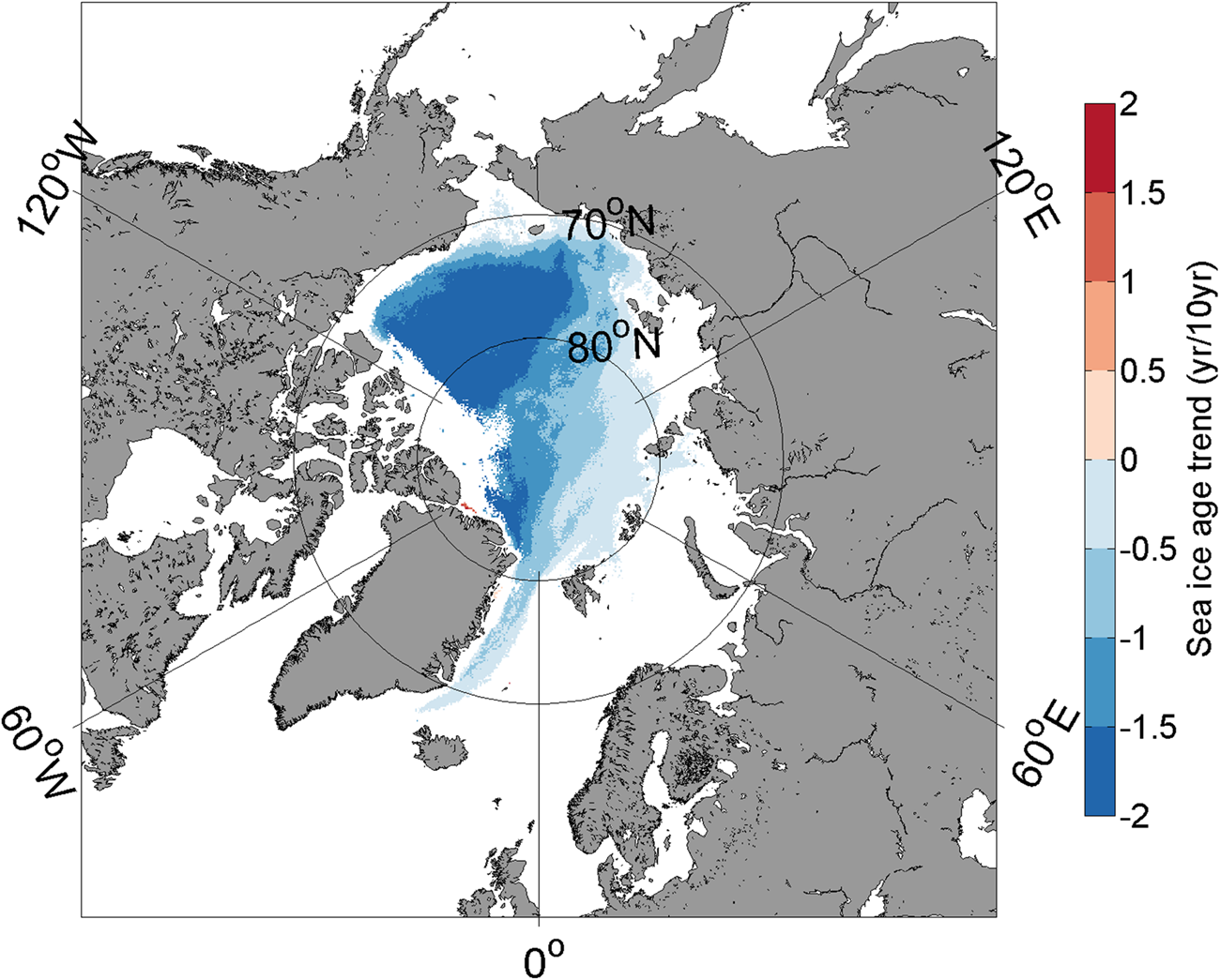
Fig. 5. Spatial distribution of the sea-ice age trend from 1984 to 2019 (coloured regions pass the significance test at the 95% confidence level) representing the transition from MYI to seasonal ice. Trends are calculated at grid points where the ice age exceeded 1 year in 1984 and then decreased to 1 year or the ice vanished.
From 2002 to 2010, the variance explained by EOF2 was 18% for AMSR-E SIC and 23% for NT SIC (Figs 3b and d). The time series of PC2 shows a robust change in 2005 (Fig. 4). The same spatial features of EOF2 are present from 2002 to 2010 and 1979–2019, and the variance explained by EOF2 from 1979 to 2019 is 7% (Fig. 3f). There is no clear trend in the time series of PC2, with several negative and positive peaks demonstrating interannual variations over the past 41 years. Morlet wavelet analysis (Torrence and Compo, Reference Torrence and Compo1998) shows that the pattern of PC2 displays significant 4–5-year periodicity from 1989 to 2012 and significant 6–7-year periodicity throughout almost the entire time series (not shown). Because the variance explained by PC2 from 1979 to 2019 is small (7%), the details will not be discussed.
3.3 Abrupt changes in WSSI from 1979 to 2019
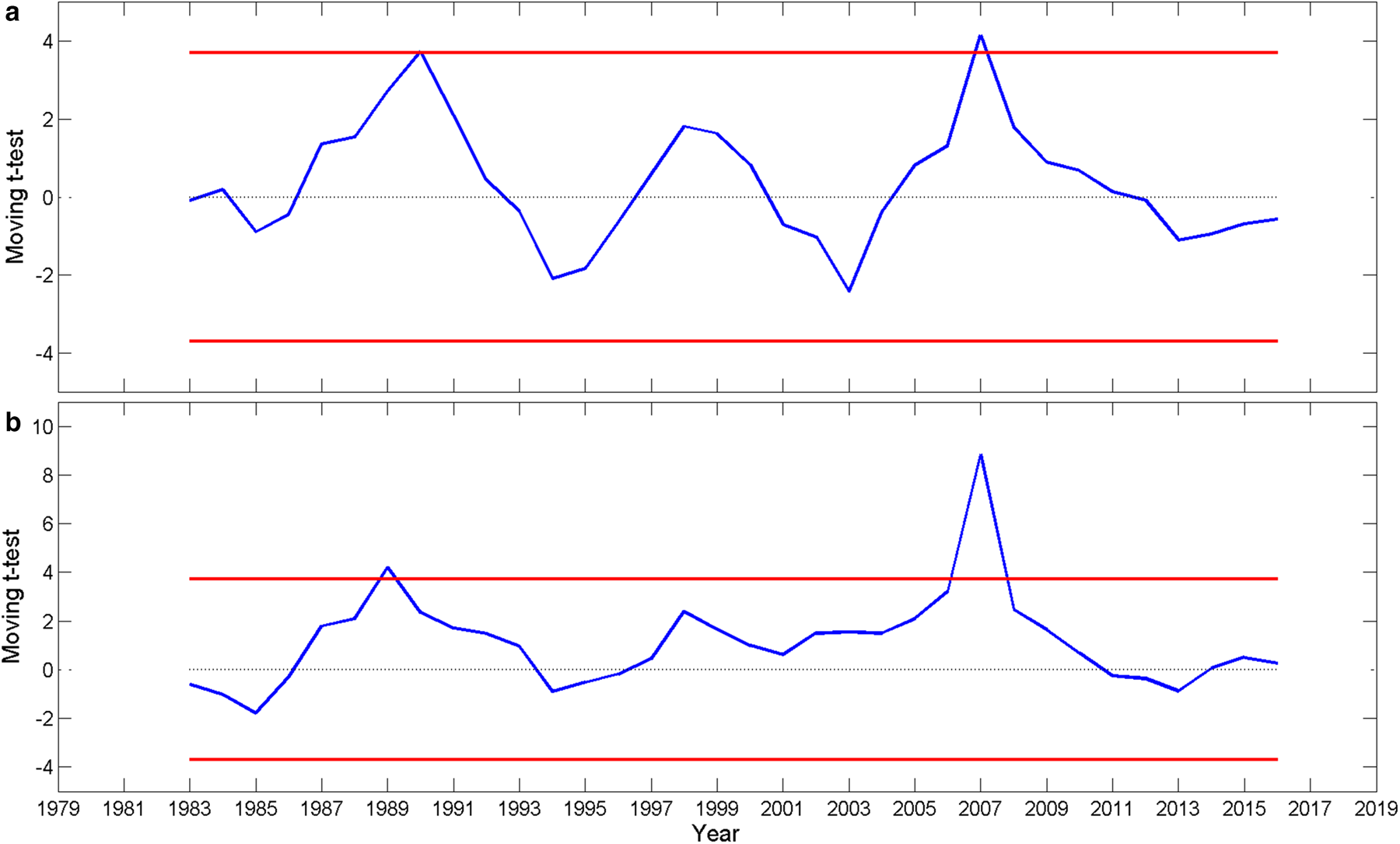
The moving t-test results for both the WSSI area anomaly and the time series of PC1 from 1979 to 2019 show a WSSI peak in 2007 (Fig. 6), as also indicated in the shorter time series from 2002 to 2010 (Fig. 4b). The time series of PC1 includes three distinct periods of negative (1979–88), neutral (1989–2006) and positive values (2007–19), as shown in Figure 4a. We focus on the shift from negative to neutral around 1989 (Figs 7a, c and e), which was linked to a phase shift of the Arctic Oscillation (AO) by Wei and Su (Reference Wei and Su2014). The change in WSSI around 1989 was, however, not as large as around 2007 (Figs 7b, d and f). The change in 2007 may have been related to the substantial decrease in September Arctic sea ice in recent decades and indicates a shift from MYI to WSSI for Arctic sea ice. This makes Arctic sea ice more liable to changes. After 2007, the Arctic sea ice extent has been even smaller in September 2012 and 2019.

Fig. 6. Moving t-test (n1 = n2 = 4) of the WSSI area anomaly (a) and the time series of PC1 (b). The blue line represents the statistical variable t and the red lines indicate the 99% confidence limits.

Fig. 7. The WSSI concentration anomaly for the years 1988–90 (a, c, e) and 2006–08 (b, d, f).
4. Variations in large-scale atmospheric circulation related to the abrupt change in WSSI
The factors that have contributed to the severe retreat of sea ice since 1989 are studied by Maslanik and others (Reference Maslanik, Serreze and Barry1996), Cavalieri and others (Reference Cavalieri, Parkinson and Vinnikov2003) and Wei and Su (Reference Wei and Su2014). In this paper, we mainly seek to determine why an abrupt increase in WSSI occurred in 2007. As the Arctic sea ice has thinned, responds to both atmospheric and oceanic forcings have increased in magnitude. Here, we focus on the atmospheric impact on WSSI. Composite analyses of Ta-500 and Z500, the vertically integrated transports of moist static energy and the jet stream properties at the 200 hPa level are performed for the periods of 1989–2006 and 2007–19, representing neutral and positive phases of PC1, respectively. For PC1, the differences between the positive and neutral phases for Z500 and Ta-500 are calculated. The analysis shows that the large-scale atmospheric circulation is correlated with the WSSI in winter (December–March), summer (July–September) and autumn (October–November). Hence, the composite analysis focuses on these seasons.
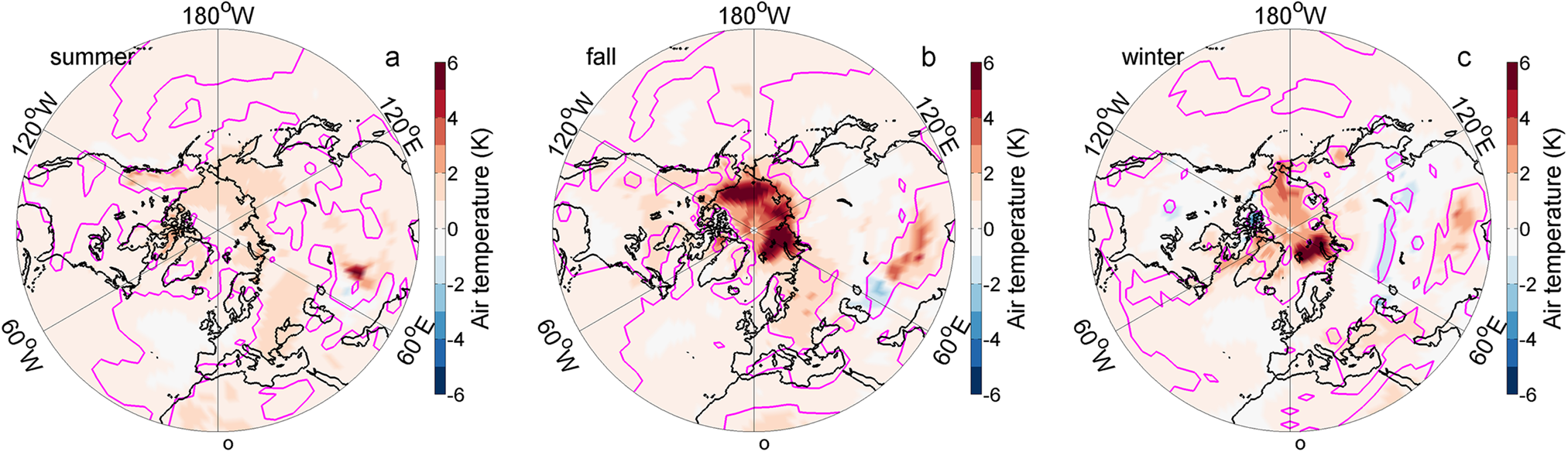
The composite fields of the anomalies of Z500 and Ta-500 show that from 1989 to 2006 (neutral phase of PC1) the anomalies compared to the entire period averaged from 1979 to 2019 (Figs 8a, e and i) are predominantly small in summer, autumn and winter (Figs 8b, f and j). On the other hand, from 2007 to 2019 (positive phase of PC1), positive anomalies occur over large regions (Figs 8c, g and k) and the anomalies show a strengthened wavenumber 3 structure, which favours the meridional transport of warm air from the south to the Pacific sector of the Arctic Ocean in summer, autumn and winter. This structure is associated with warmer anomalously low Z500 in central Siberia and anomalously high Z500 along the Arctic Ocean near the Chukchi Peninsula in summer (Fig. 8d). The high Z500 becomes stronger and moves to the central Arctic in autumn (Fig. 8h), and this pattern is associated with a warm anomaly in the Pacific sector. The differences in the surface air temperature fields demonstrate warming over the entire Arctic from summer to winter (Fig. 9). The warmer air during the period from 2007 to 2019 contributes to increased ice melt in summer and a delay in freeze-up in autumn, which results in a shorter freezing period. Hence, the seasonal ice remains thin, which results in less sea ice surviving the following melt season and less MYI in the following autumn and winter.

Fig. 8. Spatial distributions of Z500 (colours) and Ta-500 (contours, in K) during summer (July–September, left column), autumn (October–November, middle column) and winter (December–March of the following year, right column). The first row shows the average from 1979 to 2019, the second row shows the difference of 1989–2006 minus 1979–2019, the third row shows the difference of 2007–19 minus 1979–2019 and the last row shows the difference of 2007–19 minus 1989–2006. In the difference maps (second–fourth row), solid lines indicate positive Ta-500 anomalies and dashed lines indicate negative Ta-500 anomalies. The pink contours indicate the 90% significance level.

Fig. 9. Distribution of the mean surface air temperature of 2007–19 minus 1989–2006 during summer (July–September, a), autumn (October–November, b) and winter (December–March of the following year, c). The pink contours indicate the 90% significance level.
To better understand the thermodynamic importance of the Z500 fields (Fig. 8), we present results for the vertically integrated northward transport of moist static energy. Differences in the transport between the two periods (1989–2006 and 2007–19) are calculated (Fig. 10). Although these are vertically integrated values, fluxes to the Arctic peak close to the Earth's surface according to ERA-Interim data (Naakka and others, Reference Naakka, Nygård, Vihma, Graversen and Sedlar2019) have a direct effect on sea ice. Focusing on the sea-ice zone, in summer, the northward energy transport increased in the Pacific sector of the central Arctic Ocean, the East Siberian Sea, parts of the Laptev Sea and the Canadian Arctic Archipelago (Fig. 10a). In the region between Svalbard and the North Pole, the result mirrors that on the other side of the North Pole, suggesting increased transport from the Pacific Sector via the North Pole to Svalbard and farther. In autumn, the results are roughly opposite those in summer, demonstrating a strong increase in the moist static energy transport from the Atlantic sector to the North Pole and farther to the Laptev Sea and the Canadian Arctic Archipelago. In addition, the northward transport has increased in the East Siberian and Chukchi Seas (Fig. 10b). In winter, the wavenumber 3 pattern is most pronounced, with increased transport from the Barents Sea, eastern Siberia and the Canadian Arctic Archipelago to the central Arctic Ocean and decreased transport in the zones in between (Fig. 10c). A comparison of the results of WSSI trend (Fig. 1b), the surface air temperature (Fig. 9) and northward flux of moist static energy (Fig. 10), suggests that in the Pacific sector the increased northward transport of moist static energy has contributed to increased temperatures in summer (Fig. 9a) and further to enhance summer sea-ice melt. The increased northward transport of moist static energy has partly contributed to increased temperatures in autumn (Fig. 9b) and decreased autumn sea-ice growth, hence increasing the amount of WSSI. The increased northward transport of moist static energy is not perfectly aligned with the patterns of the surface air temperature because, in addition to atmospheric transport, several local feedbacks contribute to Arctic amplification (Serreze and Barry, Reference Serreze and Barry2011; Döscher and others, Reference Döscher, Vihma and Maksimovich2014; Pithan and Mauritsen, Reference Pithan and Mauritsen2014). In the Atlantic sector, our interpretation is that the strong increases in moist static energy transport in autumn and winter (Figs 10b and c) have contributed to increased temperatures (Fig. 9) and prevented sea-ice formation in regions that are covered by WSSI in previous decades, thus reducing the amount of WSSI (Fig. 1b). In addition, the northward transport of moist static energy is associated with northward winds, that push the ice edge farther north and dynamically reduce WSSI.

Fig. 10. Distribution of the vertically integrated northward flux of moist static energy of 2007–19 minus 1989–2006 during summer (July–September, a), autumn (October–November, b) and winter (December–March of the following year, c). The pink contours indicate the 90% significance level.
In the Atlantic sector, atmospheric warming is strongest in autumn and winter, which is consistent with the spatial pattern shown in EOF1; notably, the WSSI shows a decreasing trend opposite to that in the Pacific sector. In summer, strong positive Beaufort Sea High anomalies and negative geopotential height anomalies across northern Eurasia occur. These anomalies generate southerly wind anomalies and may promote strong ice melt in the East Siberian and the Chukchi Sea and promote the transport of MYI out of the Arctic Ocean via the Fram Strait (Figs 8c and d) as the ice drift pattern shows (Fig. 11). Thus, the reduced summer sea-ice cover in those regions results in more new ice formation during autumn and winter. In autumn, the positive Z500 anomaly in East Siberia controls the eastern Arctic, which may favour ice drift out of the Arctic Ocean via the Fram Strait (Fig. 11).

Fig. 11. Average sea-ice drift from 1989 to 2006 (left) and 2007–19 (right) in summer (upper panel) and autumn (bottom panel).
To better understand the factors that drive changes in the Z500 fields and the vertically integrated transport of moist static energy, we calculate the anomaly fields of 200 hPa zonal wind, which characterize anomalies in the polar front jet stream, for the periods of 1989–2006 (Figs 12b, f and j) and 2007–19 (Figs 12c, g and k). Since 2007, the core of the jet stream has become weaker in summer, fall and winter (Figs 12c, g and k), especially in the Pacific in winter. In addition, the zonal winds have become stronger north of the core of the jet stream, especially in summer. The difference between 1989–2006 and 2007–19 reflects an increasingly strong signal (Figs 12d, h and i). The weak intensity and poleward shift of the jet stream favour warmer air to flow northward, as shown by stronger-than-average northward winds in Siberia and Northern Europe in summer and autumn at 850 hPa (Figs 13a and b), which corresponds with the Z500 field (Fig. 8). Additionally, in autumn the meridional wind component at 850 hPa (Fig. 13) reflects the strengthened warm-air advection as the moist static energy (Fig. 10b) in the Pacific sector; this, together with the warm conditions in the Pacific sector (Fig. 9), limits the sea-ice growth in autumn and favours a decrease in SIC. We note that the weak polar jet stream favours the enhanced transport of warm air from the south to north (Francis and Vavrus, Reference Francis and Vavrus2015), which contribute to sea-ice melt and the Arctic amplification of climate warming. Arctic amplification is a result of complex positive feedback related to both local and hemispherical-scale processes (Serreze and Barry, Reference Serreze and Barry2011; Pithan and Mauritsen, Reference Pithan and Mauritsen2014). Hence, it is not always easy to distinguish between the cause and consequence.

Fig. 12. Spatial distributions of 200 hPa mean zonal wind (colours, in m s–1) during summer (July–September, left column), autumn (October–November, middle column) and winter (December–March of the following year, right column). The first row shows the average from 1979 to 2019, the second row shows the difference of 1989–2006 minus 1979–2019, the third row shows the difference of 2007–19 minus 1979–2019 and the last row shows the difference of 2007–19 minus 1989–2006. For all the maps, the black (yellow in the first row) contours indicate the location of the jet stream (in m s–1). The pink contours indicate the 90% significance level of the differences.

Fig. 13. Differences in the 850 hPa meridional wind component (colours, in m s−1) and wind vector of 2007–19 minus 1989–2006 (m s−1) in (a) summer (July–September), (b) autumn (October–November), and (c) winter (December–March of the following year). The pink contours indicate the 90% significance level.
5. Discussion and conclusion
In the past decades, Arctic sea ice has undergone a dramatic decline. The decreasing trends in the total Arctic sea-ice extent and area are robust, as widely discussed in previous papers (e.g. Stroeve and others, Reference Stroeve, Holland, Meier, Scambos and Serreze2007; Stroeve and others, Reference Stroeve2008; Comiso, Reference Comiso2012; Comiso and others, Reference Comiso, Meier and Gersten2017). The rapid decrease in sea ice in summer tends to result in increased WSSI. The sea-ice concentration decreases in the Arctic on average, but the change shows asymmetric and regional features (Wei and Su, Reference Wei and Su2014; Lynch and others, Reference Lynch, Serreze, Cassano, Crawford and Stroeve2016; Onarheim and others, Reference Onarheim, Eldevik and Smedsrud2018). In this study, we show that the asymmetry in ice pack evolution between the Pacific and Atlantic sectors of the Arctic Ocean is associated with increased WSSI in the Pacific sector from 1979 to 2019 (Fig. 1b). Compared to MYI, WSSI is more sensitive to atmospheric and oceanic forcing (Lynch and others, Reference Lynch, Serreze, Cassano, Crawford and Stroeve2016), as shown by the large variation in WSSI found in this study. The more WSSI instead of thick MYI in wintertime, the more open water and the greater the absorption of solar radiation in the following summer, which enhances ice-albedo feedback (Serreze and others, Reference Serreze2000) and prolongs the melt season (Stroeve and others, Reference Stroeve, Markus, Boisvert, Miller and Barrett2014).
Our analyses of WSSI variations from 1979 to 2019 confirm that two abrupt increases took place in the Pacific sector: in 1989, from a negative to a neutral phase, and in 2007, from a neutral to a positive phase of the EOF1 pattern. The pattern of EOF2 resembles that of EOF3 reported by Partington and others (Reference Partington, Flynn, Lamb, Bertoia and Dedrick2003) and EOF2 discussed by Singarayer and Bamber (Reference Singarayer and Bamber2003) and Peng and others (Reference Peng2019). The 6–7-year periodicity of the PC2 of WSSI passed the significant test at the 99% confidence level. In the Pacific sector, the ice pack has been dominated by seasonal ice since the 2007 phase shift.
The Arctic amplification of climate warming, which is strongest close to the Earth's surface, tends to weaken the jet stream in the upper troposphere, making it more meandering (Francis and Vavrus, Reference Francis and Vavrus2015); however, the effects are opposed by tropical amplification in the upper troposphere (Barnes and Polvani, Reference Barnes and Polvani2015) and the jet stream is also associated with considerable internal variability (Warner and others, Reference Warner, Screen and Scaife2020). The jet stream affects the mid- and low tropospheric synoptic-scale circulations by steering the cyclone tracks (Wickström and others, Reference Wickström, Jonassen, Vihma and Uotila2019). A highly meandering jet stream allows for the frequent occurrence of intense events associated with the transport of heat and moisture to the Arctic (Meleshko and others, Reference Meleshko, Johannessen, Baidin, Pavlova and Govorkova2016; Vihma, Reference Vihma2017). Determiningthe cause and effect relations is, however, complicated by several local and remote feedbacks (Serreze and Barry, Reference Serreze and Barry2011; Pithan and Mauritsen, Reference Pithan and Mauritsen2014). Additionally, the increased inflow from the Pacific Ocean via the Bering Strait brings heat to the Arctic and has contributed to summer ice melt and decreased winter ice growth (Woodgate and others, Reference Woodgate, Weingartner and Lindsay2012, Reference Woodgate2018). A decline in sea ice may favour the transition from a cold and stratified Arctic to a warm and well-mixed Atlantic-dominated climate regime (Lind and others, Reference Lind, Ingvaldsen and Tore2018) and cause the seasonal upwelling and downwelling of the Beaufort Gyre (Meneghello and others, Reference Meneghello, Marshall and Timmermans2018). In our results, these patterns are reflected by the increased transport of moist static energy from certain sectors to the central Arctic Ocean, demonstrating a pronounced wavenumber 3 structure, especially in winter (Fig. 10) and contributing to increasing near-surface air temperatures (Fig. 9).
The changes in WSSI show asymmetric patterns in the Pacific and Atlantic sectors. A warmer-than-average summer enhances ice melt, and warm autumn and winter seasons lead to thin ice, thus reducing the probability of ice survival following the melt season and fail to transform to MYI in the Pacific sector. Thus, WSSI increases in the Pacific sector. In winter, the warming pattern has been much stronger in the Atlantic than in the Pacific sector (Fig. 9c). This has contributed to the WSSI decrease in the Atlantic sector; notably, this region, which was previously covered by seasonal ice is now characterized by open water.
In addition to these thermodynamic effects, the changes in WSSI have been influenced by sea ice dynamics. In summer 2007, the strengthened transpolar drift of sea ice caused an increase in ice exported from the Pacific sector and the central Arctic Ocean to the Fram Strait (Zhang and others, Reference Zhang, Lindsay, Steele and Schweiger2008). Our analysis shows that the strengthened wavenumber 3 structure at high latitudes combined with a low-pressure anomaly in central and western Siberia and a high-pressure anomaly in eastern Siberia enhanced transpolar ice drift and ice transport out of the Arctic via the Fram Strait.
In summary, in this study, we (a) confirm the interannual variations in WSSI in the marginal ice zone of the central Arctic with abrupt changes in 1989 and 2007, (b) find that changes in circumpolar- and synoptic-scale atmospheric circulation (including the jet stream and wavenumber 3 pattern) and related transports of moist static energy have contributed to increases in near-surface air temperatures and thus enhance summer melt and reduce autumn/winter ice growth and (c) find that the changes in ice melt and growth have had opposite effects on the Pacific and Atlantic sectors; specifically, WSSI has increased in the Pacific sector due to replacement of MYI by WSSI, and decreased in the Atlantic sector due to the replacement of WSSI by open water.
Acknowledgements
This study was supported by the National Key R&D Program of China (Grant No. 2018YFA0605903), the Chinese Natural Science Foundation (Grant No. 41941012 and 41706223) and by the Academy of Finland (contract 317999). SIC data are provided by http://nsidc.org/data/nsidc-0051.html, NCEP/NCAR reanalysis data are from http://www.esrl.noaa.gov/psd/data/gridded/data.ncep.reanalysis.html. Sea-ice age data are from https://nsidc.org/data/nsidc-0611 and sea-ice drift data are from https://nsidc.org/data/nsidc-0116. ERA5 data are from https://cds.climate.copernicus.eu.


 Open access