


1. Introduction
The transformation of snow into ice via the process of firnification has been studied from both a theoretical viewpoint (Reference Sorge, Brockamp, Jülg, Loewe and SorgeSorge, 1935; Reference SchyttSchytt, 1958) and via empirical modelling (Schytt, 1958; Reference Langway, Shoji, Mitani and ClausenLangway and others, 1993; Reference Kameda, Shoji, Kawada, Watanabe and ClausenKameda and others, 1994). The combined outcome of these approaches has been to establish relatively simple relations equating the resultant firn density to the accumulated pressure of overlying snow layers (Schytt, 1958; Reference Herron and LangwayHerron and Langway, 1980; Langway and others, 1993). Recent empirical work has examined the additional dependence of coefficients in these relations on in situ meteorological parameters such as the annual mean temperature, as approximated by the 10 m depth firn temperature (Kameda and others, 1994). Applica-tion of these latter results to the low-accumulation, high-wind regime of the Lambert Glacier basin leads to an underestimation of density for many sites. This is attributed to wind-enhanced grain-settling effects in the upper few metres of the snowpack, especially where low accumulalion rates result in prolonged exposure to surface wind conditions.
This paper extends previous empirical work by examining also the dependence of firnification on annual mean wind speed and annual mean surface accumulation rate.
2. The Analytical Models
Two different approaches have been developed relating firn density via the porosity to overburden pressure: porosity, S, is expressed as (ρi — ρ)/ρi, where ρ is the firn density and ρ i is the bubble-free density of pure ice (taken here as 0.917 Mg m−3 at 20°C).
Assuming that snow behaves as a plastic material, the first model considers the reduction ratio of porosity (−dS/S) to increase proportionally to the increasing ratio of pressure (dP/P) and some power of the porosity. Analyzing data from Antarctica and Greenland, Kameda and others (1994) showed that this is equivalent to a proposal by Langway and others (1993) that the logarithm of the overburden pressure is proportional to the square of the porosity:
where the overburden pressure Ρ from the surface to a depth H is given by

with ρ in Mg m−3 and h the depth in metres, yielding pressure in bar. Hereafter this case is referred to as the log-squared (LS) model.
Kameda and others (1994) investigated the coefficients in this model to find a dependence of the intercept coefficient C2 on 10 m depth firn temperature, with no clear influence from annual accumulation rate. in their study, the LS model equation became:
where Τ is the temperature in K. We denote the temperature-dependent LS model as LS(T).
This equation can be used to determine the limit of applicability of the model for a given temperature, since porosity will be zero for a density equal to the bubble-free density of pure ice. For a temperature of -20°C the maximum overburden pressure is 3.48 bar, corresponding to a depth of approximately 53 m. in practice, the LS(T) model breaks down earlier than this, which is not altogether unexpected given that viscous flow enters considerations before such a point is reached. Thus the model has a high-density-breakdown regime built into it by virtue of the empirically determined exponent of the porosity in the original perfect-plasticity assumption.
A second firn-densification model relates the reduction ratio of porosity to the increment of pressure and some power of the porosity. Kameda and others (1994) showed a best fit for a zero exponent, which is equivalent to the original proposal of Schytt (1958) and leads to an equation where the overburden pressure is related to the logarithm of the porosity:
We refer to this as the linear-log (LL) model.
In this formulation Kameda and others (1994) found a dependence of the gradient term C 3 on the 10 m firn temperature yielding the LL(T) empirical model:
The logarithm of the porosity forces this function to asymptote toward the bubble-free density of pure ice so that the LL(T) model may better predict behaviour at greater depth.
Kameda and others (1994) found it necessary to exclude data from two sites when determining the coefficient dependences in Equations (2) and (4). One site in Greenland was located in a percolation zone; the other was Mizuho Station, Antarctica, a low-accumulation-rate site with high katabatic winds which had denser layers at the surface than either model predicts.
The interior of the Lambert Glacier basin is a low-accumulation region where the processes of surface-snow redistribution under the influence of a strong katabatic-wind regime dominate the accumulation pattern (Reference Goodwin, Higham, Allison and JiawenGoodwin and others, 1994). This is most evident at station LGB35 at the southern extremity of an Australian National Antarctic Research Expedition (ANARE) traverse line which semi-circumnavigates the basin (Reference Higham, Craven, Ruddell and AllisonHigham and others, 1997). At this site annual wind speed is 11.3 m s−1, with a 30 km smoothed average accumulation rate of only 0.039 m a−1 w.e. These characteristics are similar to those at Mizuho Station, some 20° longitude to the west. As a result, both LS(T) and LL(T) models grossly underestimate the increase of density with depth for LGB35 (fig. 1a).
Density in the top few metres of core is highly variable. This is due to the development of intermittent layers of depth hoar in temperature gradients formed beneath
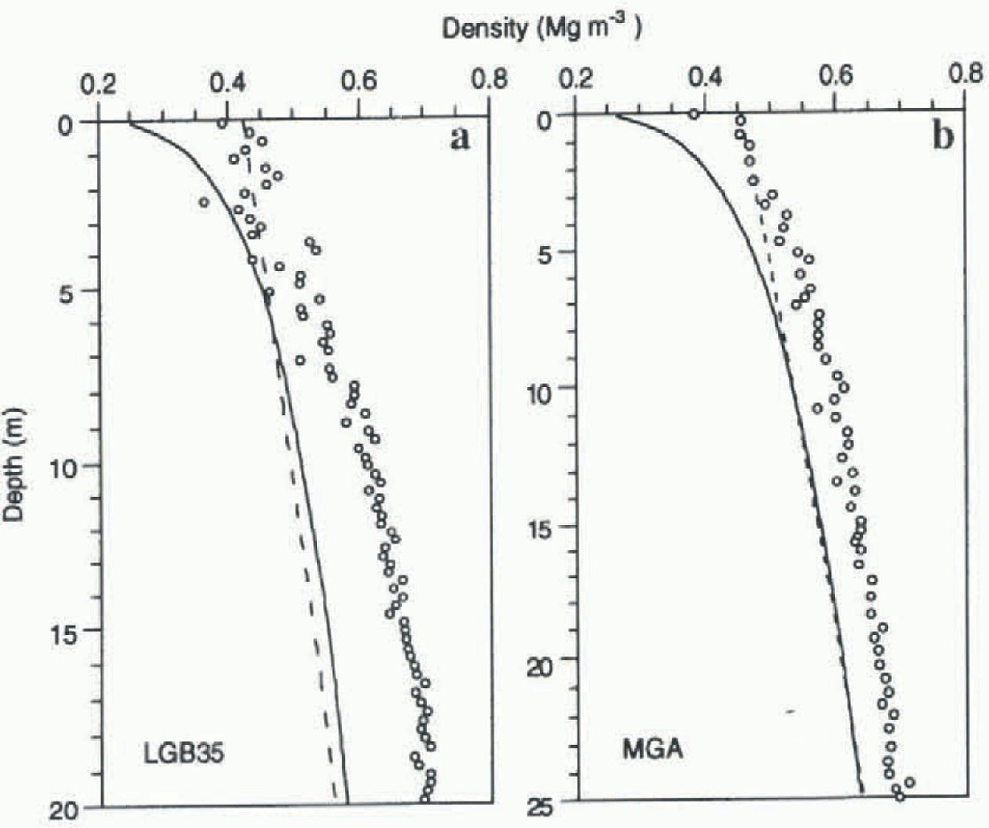
Fig. 1. Density-depth profiles fir (a) LGB35 and (if) MGA against temperature-dependent LS(T) (solid line) and LL(T) (dashed line) models.
strongly glazed surface-wind crusts characteristic of the area (Higham and others, 1997). The overall effect of the strong-wind regime, however, is to enhance grain-settling rates in the upper few metres of the pack. This is the predominant mechanism during the first stage of firnification up to densities around 0.55 Mgm −3 (Reference PatersonPaterson, 1994).
Station MGA, situated on the coastal slopes west of the basin, has a mean annual wind speed similar to LGB35 but a considerably higher accumulation rate of 0.250 m a−1 w.e. Density predictions from both models again underestimate true densities, but by only about half the extent of that at LGB35 (fig. 1b). Clearly, the extra thickness of the added annual layers moderates the enhanced packing due to the high-wind regime for the area.
3. Empirical Results
Kameda and others (1994) found significant correlation for coefficients C-2 and C3 with 10 m firn temperature only. The high-wind-regimc, low-accumulation-rate Mizuho Station was excluded from their analysis. These relationships have been re-examined using both old and new field data from
Table 1. Site locations and annual mean meteorological data

Table 2. Linear correlation analysis for LS and LL models
ten Antarctic sites of widely varying location and physical characteristics (table 1). Maudheim and Gl (Amery Ice Shelf) which are used later to test the results are also shown.
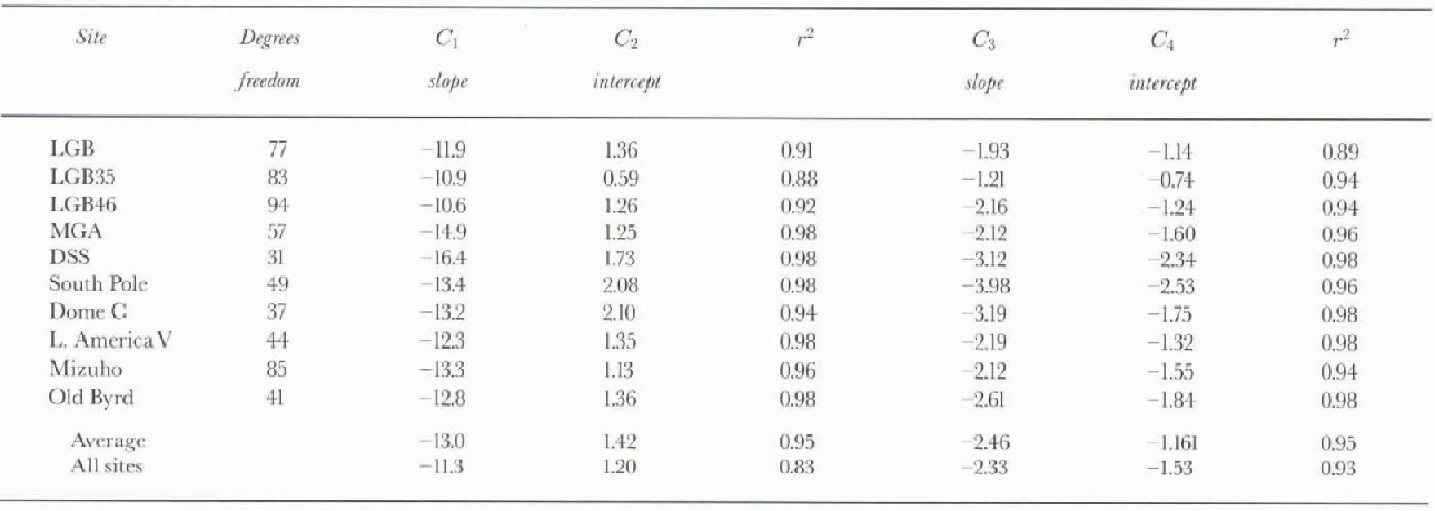
A linear correlation analysis was firstly carried out on measured densities from cores from each of the ten sites, to determine slope and intercept coefficients for the two models without any dependence on meteorological parameters (Equations (1) and (3)). The results are shown in Table 2. Four of the sites are the same as those used by Kameda and others (1994), and the coefficients for these are taken directly from that paper. As previously indicated, the LS model breaks down for higher densities, so data points for S2 < 0.01 (ρ> 0.825 Mg m −3) are excluded from the least-squares calculations.
For individual sites the r2 values averaged 0.95 for both models. When model fits were carried out on combined data from all sites, the LS model produced an r2 value of 0.83. figure 2a indicates that, although overburden pressure is the dominant influence, other factors exert secondary effects, particularly on the intercept C 2. For the LL model the r2 value of 0.93 was marginally below the average for individual sites, indicating that secondary influences were relatively minor. As shown by Kameda and others (1994), the slope coefficient C 3 varies from site to site for this model (fig. 2b).
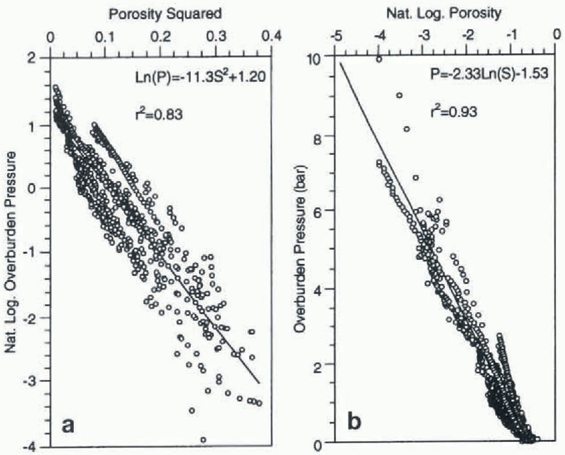
Fig. 2. Combined data from all sites showing intercept variation of LS model (a) and slope variation of LL model (b).
To assess effects of site meteorological parameters (10 m depth firn temperature, mean annual wind speed and mean annual accumulation rate) on the LS model, we performed a multivariate analysis on C2 whilst holding C1 constant.
This multiple regression (LS(TWA) model) resulted in:
when- Τ is temperature in K, W is wind speed in m s and A is accumulation rate in m a−1 w.e. The coefficient of determination (r2) for the multiple regression involving C2 intercept data from the ten sites was 0.83. The F statistic of 9.46 is approximately equal to the P-critical value of 9.78 at the 99% confidence level for a regression with ten data points and three variables. Coefficients for the three independent variables (temperature, wind and accumulation rate) and the constant term all yielded Student t variables at the 90-95% confidence level.
For the LL model, similar multivariate analysis of the slope coefficient C 3 was carried out whilst the intercept coefficient C4 was held fixed. This resulted in an LL(TWA) model where :

with an r2 of 0.50 and an P-observed of 1.96, marginally above the P-critical value of 1.78 at the 75% confidence level. Individual i-test values for temperature, wind and accumulation rate were as low as 85%, 55% and 80%, respectively.
Without wind-speed dependence (LL(TA) model), the regression resulted in:
with r2 — 0.44, an Ρ statistic marginally below a 90% confidence level, with temperature, accumulation-rate and constant-term dependences all above a 90% confidence level.
4 Comparison With Data
Density—depth profiles together with model predictions, including the temperature, wind and accumulation-rate effects, are shown in Figure 3. Curves for LGR35 and MGA can be compared with Figure 1.

Fig. 3. Density-depth profiles for the ten sites used to derive the model coefficients, plotted against model predictions (LS(TWA), solid line; LL(TWA), long dashes; LL(TA), short dashes). Data for South Pole and Old Byrd were provided as smoothed densities over 1 m intervals. Test sites Maudheim and G1 (Amery Ice Shelf) appear in the last two frames.
4.1. LS model
The original Kameda and others (1994) LS(T) model severely underestimates firnification rates with in the snow-pack for low-accumulation-, high-wind-regime sites such as Mizuho Station and LGB35. LS (TWA) clearly resolves this mismatch (Fig. 3), producing more realistic densities in the top 30 m of firn, beyond which the model begins to fail as densities exceed 0.75 Mg m −3. Breakdown of the LS models at high density occurs for all sites; the meteorological variables merely delermine the depth at which the breakdown occurs.
LS (TWA) model predictions match density-depth profiles in the upper layers for a wide range of conditions: high wind, low accumulation at Mizuho and LGB35; high wind, high accumulation at MGA; low wind, low accumu-lation at Dome C, South Pole, LGB20 and LGB46; and low wind, high accumulation at Little America V, Old Byrd and Maudheim. LS(T) accounted for measured profiles at Dome C, Old Byrd and Little America V also, but not for lire Mizuho core. The balance between all three variables as in the LS(TWA) model accounts for a wider range of local conditions. However, LS(TWA) still underestimates densities for DSS (Law Dome) inW'ilkcs Land. DSS experiences moderate winds but extremely high accumulation rates compared to all other sites in this study (table 1). This indicates that cores from other high-accumulation sites could be used to refine the model further so it provides an even better fit to field data.
The density-depth profile for G1 (Amery) exhibits an unusual trenti nol evident in other t ores (except possibly in Little America V). One interpretation is that the core follows one firnification profile for the first 15 m, then migrates to another from around the 30 m mark. Several possibilities exist for this. Firstly, G1 at the time of coring was situated some 70 km from the front of the Amery Ice Shelf. It may be that local snow undergoing firnification is laid down on top of continental ice transported down the glacier ice-shelf system. This is in fact true, but the shelf-ice-continental-ice interface is not reached until about 70m (Reference MorganMorgan, 1972). Another possibility is that the firnification process is responding to two distinct periods of quite different accumulation rate and/or temperature. The upper 15 m may reflect the current rate (being 1968 when the core was collected) of 0.35 m a−1 w.e., while the lower parts of the core indicate an earlier, lower rate, perhaps of the order of 0.20 m a−1 w.e. Such a dramatic accumulation-rate increase is not supported by other data. Alternatively, the deeper core section may correspond to a warmer period of increased melt and higher ablation, which in turn strongly enhance firnification rates ( Paterson, 1994), as has been interpreted for the Amery in recent times (Goodwin, 1995). This need not be reflected in the annual mean temperature, but may result from warmer than usual summers with percolation affecting deeper parts of the core as well. Little America V, another near-front ice-shelf site, shows a similar feature around 40 m depth (fig. 3g) where the density increases sharply for a period. Such transitions may be characteristic of profiles at similar low-elevation sites where small temperature fluctuations have a large relative effect on freeze/melt rates, though this feature is not evident in the Maudheim core.
4.2. LL model
All models, LL(T) (Kameda and others, 1994), LL(TWA) and LL(TA), had mixed success in matching the data in detail, but produced realistic trends at depth ( figs 1 and 3).
LL(TA) was best for low-accumulation sites except LGB46. At high-accumulation sites the model predictions fit the data for the high-wind site MGA, but overestimate densities elsewhere, apart from the extremely high-accumulation site DSS. LL(TWA) matched MGA (high wind, high accumulation) and Dome C (low wind, low accumulation) quite well, but generally overestimated elsewhere. Given reduced confidence levels in the regression analyses, this is not altogether surprising. At least the inclusion of accumulation rate (with or without wind) can be seen to affect the modelled results considerably.
5. Discussion
5.1. Sensitivity of models to step size
The equation for the LS model cannot be solved analytically. A stepwise numerical iteration is used to obta in the density at any given depth. Effectively, the overburden pressure is calculated using the sum-product of all preceding densities and their associated core-depth increments.
Sensitivity tests were carried out to examine the dependence of the calculated density-depth profile on the increment step size in depth. figure 4a shows the results for the LS(T) model using depth increments of 0.01,0.1,0.25,0.5 and 1.0 m at a representative temperature of -30°C.The smaller the step size, the closer the curve approximates an ideal, continuously integrated density-depth profile. in reality, particularly near the lop of a core, the density increases in stepwise rather than continuous fashion. The error introduced by a change in step size from 1.0 m to 0.01 m is of the order of 6% at a depth of 2 m and only 2% by the time 10 m is attained. These errors are negligible with respect to the variation in real data and the physical errors involved in the measurement itself. Where the variable observed data increments have not been used, a step size of 0.25 m has been chosen as a representative magnitude in calculating the model curves.
Similar arguments apply to the LL(T) model) where the error margins are smaller and nearly linear with depth, as shown in figure 4b.

Fig. 4. Sensitivity tests for (a) LS(T) model and (b) LL(T) model, showing dependence on computational step size.
5.2. LS model sensitivity to temperature, wind and accumulation rate
figure 5a is a set of nomograms which illustrates the sensitivity of the LS(TWA) model to wind speed at a nominal temperature of -20°C and accumulation rate of 0.15 m a−1 w.e. An increase/decrease in temperature of 10°C equates to a wind-speed increase/decrease of approximately 5ms−1, as shown by the fine dashed curves in figure 5a. Similarly, an increase/decrease in accumulation rate of 0.05 m a−1 w.e. equates to a wind-speed decrease/increase of approximately 2.5 m s−1. figure 5b presents a similar set of curves for a nominal temperature of-20°C at a wind speed of 5 m s −1 for a range of accumulation rates. An increase/decrease in annual mean temperature of 10° C equates to a decrease/ increase in accumulation rate of 0.10 m a−1 w.e. These figures are a guide to inter-site comparison.
Beyond 0.70-0.75 Mg in , predicted density changes do not match real changes with in the snowpack (fig. 5a and b). Predictions for the depth at which pore close-off occurs (0.83 Mg m −3; Paterson, 1994), are likely to be too shallow. LGB35 and Mizuho provide clear examples of this, where the LS(TWA) model predicts first-stage depths (0.55 Mgm−3) close to those observed, but cut-off depths several metres too shallow (table 3).
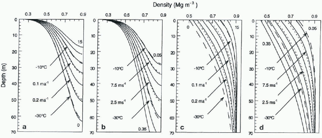
Fig. 5. Density-depth nomograms fir LS(TWA) model, showing (a) effect at -20°C and 0.15 ma−1 of winds from 0.0 to 15.0 m s −1 in steps of 2.5ms ' and (b) accumulation ratefrom 0.05 to 0.35 m a−1 in steps of 0.05 ma−1 for -20a C and 5.0 ms−1. Effects of varying either temperature (long dashes) or accumulation/wind rate (short dashes) are also shown. Similarly for LL(TWA) model (c,d).
5.3. LL model sensitivity to temperature, wind and accumulation rate
Simple rearrangement of the LL(TWA) model leads to an iterative formulation which asymptotes toward the density of bubble-free pure ice.
figure 5c and d indicate that temperature and accumulation rate have the greatest influence on the LL profiles. An increase/decrease of 10°C equates to an increase/decrease in wind speed of approximately 7.5 m s−1, and a decrease/ increase in accumulation rate of approximately 0.10m a−1 w.e. An increase/decrease in wind speed of 2.5 m s −1 matches a decrease/increase in accumulation rate of 0.04 m a−1 w.e.
This model generally produces densities at the surface which are much higher than observed. This feature of the model, along with its asymptotic approach to the density of pure ice, indicates that it is more applicable to the second stage of firnification, from 0.55 to 0.83 Mg m 3, and beyond. Predicted depths of the first stage of firnification and the transition density from firn to glacier ice are given in Table 3.
6. Conclusions
The results presented here confirm that Antarctic firn den-
Table 3. Depth of first (0.55 M gm −3) and second (0.83 Mg m −3) stages of firnification at selected sites for the various models ( dashes indicate surface densities above this limit)

sities are predominantly determined by overburden pressure and that variability among sites is governed by local meteorological parameters: temperature, wind and accumulation rale. For the first and early second stages of firnification, up to around 0.70-0.75 Mg m−3, an LS model provides an adequate description of the process. Increased temperatures and stronger surface winds enhance firnification, whilst higher accumulation rates mask these effects by limiting the length of time for which the upper layers are exposed to surface conditions. For the second stage, through to densities approaching the maximum limit of pure ice, an LL model provides the better match with data. Temperature is an important factor in this model, and accumulation rate appears to be a significant parameter as well, though surface wind speed has minimal influence at depth. Stepwise transitions in density depth profiles may be a recurrent feature in cores taken from sites located near the fronts of large ice shelves due to periods of melt and ablation which strongly influence densities beyond the applicability of the models presented here.
Acknowledgements
The authors would like especially to thank O. Watanabe, T. Kameda and the National Institute of Polar Research, Tokyo, for their kind assistance in furnishing meteorological measurements and density-depth data from a range of cores used in their earlier studies. We gratefully acknowledge the valuable contribution from workers of many nations who gathered data and core samples in the field. We would like to thank ANARE personnel and Australian Antarctic Division staff who contributed to the Lambert Glacier-Amery Ice Shelf project over many years. I. Goodwin, V. Morgan, A. Ruddell and M. Ross provided much helpful discussion.


