2.1 Glossary of Terms

• n = Local navigation frame of axes

• b=Real body frame of axes

• b* = Computed body frame of axes

• C_a^b = Direction cosine transformation between a-frame and b-frame

• v = Velocity, m/s

• a = Acceleration, m/s²

• ψ = Attitude angle

• ∇ = Instrument error vector of accelerometers

• ε = Instrument error vector of gyros

• Δx = Variable displacement vector

2.2. Formulations

In Kain and Cloutier (Reference Kain and Cloutier1989), the framework of TA via velocity matching is presented by the following differential equations:

(1)$${\rm \Delta} {\bf \dot v} = {\rm \Delta} \psi \times C_{b^ *} ^n {\bf a}_s^b + C_{b^ *} ^n ({\bf a}_{\,fb}^b + \nabla _a^b),$$

(2)$${\rm \Delta} \dot \psi = C_{b^ *} ^n (\omega _{fb}^b + \varepsilon _g^b ),$$

where:

• Δv is velocity difference between the master and slave velocities.

• Δψ denotes the ‘misalignment’ of the slave INS b*-frame from the ‘true’ North-East-Down (n-frame).

• C_b*ⁿ is the estimated body-to-navigation frame direction cosine transformation.

• a_fb^b denotes the flexible body acceleration which is equal described by a stochastic process.

• ∇_a^b and ε _g^b are parameterized instrument error vectors of accelerometer and gyros, respectively.

• ω _fb^b is the flexible body rotation rate.

As pointed out (Britting, Reference Britting1971; Itzhack and Porat, Reference Itzhack and Porat1980; Yi, Reference Yi1987 and Wendel et al., Reference Wendel, Jurgen and Gert2004), the accelerometer and gyro instrument error parameterization is very complex for accurate modelling. However, most literatures consider the random error of gyros as a mixture of three independent elements that will be referred to hereafter as successive start drifting ε _bi, random walk ε _ri and white noise signals w _g. Consequently, ε _bi and ε _ri can be formulated as:

(3)$$\dot \varepsilon _{bi} = 0\quad\hskip42pt i = x,y,z,$$

(4)$$\dot \varepsilon _{ri} = \displaystyle{{ - 1} \over {\tau _g}} \varepsilon _{ri} + w_{ri} \quad i = x,y,z,$$

where τ _g means the correlated time of gyros' output.

The total error of gyro is:

(5)$$\varepsilon _g = \varepsilon _b + \varepsilon _r + w_g. $$

The instrument error of accelerometer ∇ is modelled as a mixture of random constant ∇_b and white noise w _a:

(6)$$\nabla _i = \nabla _{bi} + w_{ai} \quad i = x,y,z,$$

where $$\dot \nabla _{bi} = 0,i = x,y,z$$.

Generally speaking, the commonly selected states include ∇v, ∇Ψ, ε_gi and ∇_i, i=x, y, z. It is worth noting that some additional states can also be augmented into other TA models. However, for simplicity, those states are not involved in this paper.

Let be the lever-arm vector denoting the relative distance between the SINS with respect to the MINS. Then the relationship between velocity of the MINS and the SINS can be shown (Sun and Deng, Reference Sun and Deng2009), as:

(7)$${\bf \tilde v}_s^n = {\bf v}_m^n + \omega _{en}^n \times {\bf \tilde r}^n + {{\hskip3pt\bf \dot \tilde\hskip-2pt r\hskip1pt}^n + \delta v,$$

where r + δr.

The lever-arm compensation on the velocity output of the MINS can be calculated as follows:

(8)$${\bf v}_m^{comp} = {\bf v}_m^n + C_a^n [(\omega _{ia}^a - \omega _{ie}^a ) \times {\bf r}^a ].$$

Then the measurement equation for velocity matching case in traditional TA takes the following form:

(9)$${\bf Z}_v = {\bf \tilde v}_s^n - {\bf v}_m^{comp} = \Delta {\bf v} + C_a^n (\omega _{ea}^a \times )\delta {\bf r}^a + \upsilon _v, $$

where:

• $$\upsilon _v = C_a^n {\hskip4pt\bf \dot \tilde\hskip-2pt r\hskip1pt}^a $$ and can be seen as white measurement noise.

• δ r represents the lever-arm error vector and can be modelled as random constants.

Then, the traditional TA model consists of Equations (1)–(6) and Equation (9). Based on this traditional formulation, the objective of this paper is to obtain an equal TA framework with uniform observability.

3.1 Constrained Descriptions of Instrumental Errors and Lever-Arm

Without loss of generality, the random walk component in Equation (4) is widely accepted as a first-order Gauss-Markov process. Suppose the inertial outputs are sampled with unit interval, the correspondingly discrete model can be written as:

(10)$$\varepsilon _r (k + 1) = \displaystyle{{\tau _g - 1} \over {\tau _g}} \varepsilon _r (k) + w_r (k + 1),$$

(11)$$w_r (k + 1)\sim {\bf N}(0,\sigma _r^2 ),$$

(12)$$\varepsilon _b (k + 1) = \varepsilon _b (k),$$

(13)$$w_g (k + 1)\sim {\bf N}(0,\sigma _w^2 ),$$

The correlated time of gyros τ _g is generally longer than several hundreds of seconds. Substituting Equations (10)–(13) into Equation (5) yields:

(14)$$\varepsilon _g (k + 1) = \varepsilon _r (k + 1) + \varepsilon _b (k + 1) + w_g (k + 1)\sim {\bf N}(\varepsilon (k),(\sigma _r^2 + \sigma _w^2 )).$$

Similarly, the accelerometer error in Equation (6) can be rewritten as:

(15)$$\nabla (k) = \nabla _b + w_a (k)\sim {\bf N}(\nabla _b, \sigma _a^2 ).$$

It is worth noting that the above instrumental errors are represented in the slave body frame. Because the established instrumental error model varies with inertial instruments and modelling methods, for simplicity, we only consider a well-accepted instrumental error model here. However, it is easy to extend this constrained description framework to other error models.

On the other hand, the effects of lever-arm motion and ship flexure remarkably confine the alignment accuracy and rapidity in the presence of ship-dynamics, which are rather difficult to compensate due to their strong uncertainties (Titterton and Farnborough, Reference Titterton and Farnborough1990). In this section, we suggest that the lever-arm can also provide auxiliary information to evaluate the initial misalignment-states. As depicted in Figure 1, the coupled relationships of relative velocity and angular rotation between the MINS and SINS in the presence of dynamic deformation can be equally described as a group of constraints.

Figure 1. Coupled constraints description from lever-arm effect.

The relationship between relative linear velocity and angular velocity is well known as:

(16)$$(\omega _s^n - \omega _m^n ) \times {\bf r}^n = ({\bf v}_s^n - {\bf v}_m^n ),$$

where ω _sⁿ can be arranged as:

(17)$$\{ [I + ({\rm \Delta} \psi \times )]C_b^{n^ *} (\tilde \omega _s^b ) - \omega _m^n \} \times {\bf r}^n = {\rm \Delta} {\bf v}.$$

Equations (14), (15) and (17) constitute the constrained descriptions of instrumental errors and lever-arm effect. The CTA model can be summarized as the following discrete-time form:

(18)$${\bf X}(k + 1) = {\bf AX}(k) + {\bf Gw}(k),$$

(19)$${\bf Z}(k){\rm} = {\bf HX}(k) + \upsilon (k),$$

subject to:

(20)$${\bf w}(k)\sim {\bf N}\left( {\left[ {\openup3\matrix{ {\varepsilon _g (k - 1)} \cr {\nabla _b} \cr}} \right],\left[ {\matrix{ {\sigma _r^2 + \sigma _w^2} & 0 \cr 0 & {\sigma _a^2} \cr}} \right]} \right),$$

(21)$$\upsilon (k)\sim {\bf N}(0,\sigma _m^2 ),$$

(22)$$\Delta {\bf v} = \{ [I + (\Delta \psi \times )]C_b^{n^ *} (\tilde \omega _s^b ) - \omega _m^n \} \times {\bf r}^n, $$

where:

• X = [Δψ _x, Δψ _y, Δψ _z, Δv _x, Δv_y, Δv _z]^T (n − frame).

• G= diag(C _b*ⁿ, C _b*ⁿ), σ _m² is the covariance of measurement noise.

• w = [ε _gx, ε_gy, ε_gz, ∇_x, ∇_y, ∇_z] (b − frame) and A is derived by traditional TA model described in Equations (1) and (2).

3.2. Observability Analysis on TA Models

It is worth noting that the observability analysis of dynamic time-varying systems is still an open question. On the basis of observability analysing methods (Ham and Brown, Reference Ham and Brown1983; Meskin and Itzhack, Reference Meskin and Itzhack1992a; Reference Meskin and Itzhack1992b), the observability analyses on traditional TA models were referenced in many previous literatures (e.g., Jiang and Lin, Reference Jiang and Lin1992; Fang and Wan, Reference Fang and Wan1996). Generally speaking, the velocity and angular misalignment can be easily observed under proper measurement model, and it is hard to observe all the instrumental error uniformly at the same time. In this section, the observability analysis is introduced in the proposed CTA system.

Meskin and Itzhack (Reference Meskin and Itzhack1992a; Reference Meskin and Itzhack1992b) have pointed out that the observability analysis of the time-varying alignment system at the j^th segment, after having gone through segments 1, 2,…, j − 1, has to be carried out on $${\bf \tilde Q}_j $$, the Total Observability Matrix (TOM) at that segment. The matrix $${\bf \tilde Q}_j $$ is constructed as follows:

(23)$${\bf \tilde Q}_j = \left[ {\openup4\matrix{ {{\bf \tilde Q}_1} \cr {{\bf \tilde Q}_2 e^{{\bf A}_{\bf 1} \Delta _{\bf 1}}} \cr {\ldots} \cr {{\bf \tilde Q}_j e^{{\bf A}_{{\bf j} - {\bf 1}} \Delta _{{\bf j} - {\bf 1}}}\ldots e^{{\bf A}_{\bf 1} \Delta _{\bf 1}}} \cr}} \right],$$

where:

$${\bf \tilde Q}_i^T = \left[ {\matrix{ {{\bf H}_i^T |({\bf H}_i {\bf A}_i )^T |({\bf H}_i {\bf A}_i^2 )^T |\ldots|({\bf H}_i {\bf A}_i^{n - 1} )^T} \cr}} \right],1 \leqslant i \leqslant j$$, can be seen as the discriminant matrix of observability according to the classic control theory in the instantaneous case.

Δ_i is the time span of segment i.

Furthermore, the TA models constitute dynamic systems for which Theorem 2 in (Meskin and Itzhack, Reference Meskin and Itzhack1992a; Reference Meskin and Itzhack1992b) holds, thus we can use the Stripped Observability Matrix (SOM) $${\bf \tilde Q}_s (\,j)$$ for simplicity. The SOM is constructed as:

(24)$${\bf \tilde Q}_s (\,j) = \left[ {\openup3\matrix{ {{\bf \tilde Q}_1} \cr {{\bf \tilde Q}_2} \cr {\ldots} \cr {{\bf \tilde Q}_j} \cr}} \right].$$

For the constrained TA model in Equations (18)–(22), the instantaneous discriminant matrix in segment i is:

(24a)$${\bf \tilde Q}_i^T = \left[ {\matrix{ {{\bf H}_i^T |({\bf H}_i {\bf A}_i )^T |({\bf H}_i {\bf A}_i^2 )^T |\ldots|({\bf H}_i {\bf A}_i^5 )^T} \cr}} \right]$$

where:

$$\openup4\eqalign{H = & \left[ {\matrix{ {{\bf 0}_{3 \times 3}} & {{\bf I}_{3 \times 3}} \cr}} \right] \cr A = & \left[ {\matrix{ {A_{11}} & {A_{12}} \cr {A_{21}} & {A_{22}} \cr}} \right],\quad A_{12} = \left[{\matrix{ 0 & {\displaystyle{{ - 1} \over {R + h}}} & 0 \cr {\displaystyle{1 \over {R + h}}} & 0 & 0 \cr {\displaystyle{{\tan L} \over {R + h}}} & 0 & 0 \cr}} \right],\quad A_{21} = \left[ {\matrix{ 0 & { - f_u} & {\,f_n} \cr {\,f_u} & 0 & { - f_e} \cr { - f_n} & {\,f_e} & 0 \cr}} \right]$$

$$\openup4\eqalign{ A_{11} = & \left[ {\matrix{ 0 & {\omega _{ie} \sin L + \displaystyle{{v_e \tan L} \over {R + h}}} & { - \left(\omega _{ie} \cos L + \displaystyle{{v_e} \over {R + h}}\right)} \cr { - \left(\omega _{ie} \sin L + \displaystyle{{v_e \tan L} \over {R + h}}\right)} & 0 & {\displaystyle{{ - v_n} \over {R + h}}} \cr {\left(\omega _{ie} \cos L + \displaystyle{{v_e} \over {R + h}}\right)} & {\displaystyle{{v_n} \over {R + h}}} & 0 \cr}} \right] \cr A_{22} = & \left[ {\matrix{ {\displaystyle{{v_n \tan L - v_u} \over {R + h}}} & {2\omega _i e\sin L + \displaystyle{{v_e \tan L} \over {R + h}}} & { - \left(2\omega _{ie} \cos \lambda + \displaystyle{{v_e} \over {R + h}}\right)} \cr { - 2\left(\omega _{ie} \sin L + \displaystyle{{v_e \tan L} \over {R + h}}\right)} & {\displaystyle{{ - v_u} \over {R + h}}} & {\displaystyle{{ - v_n} \over {R + h}}} \cr {2\omega _{ie} \cos L + \displaystyle{{v_e} \over {R + h}}} & {\displaystyle{{2v_n} \over {R + h}}} & 0 \cr}} \right]} $

Please refer to (Britting, Reference Britting1971) for details on the above notations. We can easily find that the rank of the SOM is uniformly equal to six even without any manoeuvring motion, which equally means that the constrained system is completely observable in every segment. See (Rao et al., Reference Rao, Rawlings and Mayne2003) for detailed definitions of observability.

3.3 Moving Horizon Estimator and its Modified Version in CTA Case

When it comes to the constrained estimation problem, various filters other than traditional Kalman filtering have been presented (Simon, Reference Simon2010), such as projecting methods, unscented filtering and truncated particle filtering, etc. To maintain a trade-off between accuracy and calculating costs, the MHE (Muske and Rawlings, Reference Muske and Rawlings1993), which stems from the Bayesian Maximum a Posterior (MAP), is modified to better suit the proposed framework. The Bayesian MAP estimation of x given y essentially means the most likely value of x, given y is:

(25)$$\hat x_{map} = arg\mathop {\max} \limits_x p(x\,|\,y)$

Essentially speaking, MHE is an approximation of MAP estimation with a moving, fixed-size estimation window. The fixed-size estimation window is necessary to bound the size of the quadratic program. Most previous works assume that the noise among the system is mutually independent and the initial state and noise have (truncated) Gaussian distributions with zero means, where the posterior probability can be easily derived (Muske and Rawlings, Reference Muske and Rawlings1993; Goodwin and Hernan, Reference Goodwin and Hernan2004), while in the CTA case as proposed in Equations (18) and (19), we take the varying means Gaussian distributions into account. That is:

(25a)$$\eqalign{& p_{w(k)} (w) \propto exp\left\{{ - \displaystyle{1 \over 2}[w - w(k - 1)]^T Q_k^{ - 1} [w - w(k - 1)]}\right\} \right, \cr & p_{\upsilon (k)} (\upsilon ) \propto exp\left( - \displaystyle{1 \over 2}\upsilon ^T R_k^{ - 1} \upsilon \right), \cr & p_{X(0)} (X) \propto exp\left[ - \displaystyle{1 \over 2}\left( X - \overline {X_0}\hskip1pt \right)^T P_0^{ - 1} \left(X - \overline {X_0} \right)\right],} $$

where R, Q and P ₀ are the covariance matrix of measurement noise, system noise and error covariance of initial states, respectively.

Using Bayes' rule, we have (Rao, Reference Rao2000)

(26)$$\eqalign{& p(x_0,\ldots, x_T |y_0,\ldots, y_{T - 1} ) \propto p_{x_0} (x_0 )\prod\limits_{k = 0}^{T - 1} {\,p_{v_k}} (y_k - h_k (x_k ))p(x_{k + 1} |x_k ), \cr & p(x_{k + 1} |x_k ) = p_{w_k} (x_{k + 1} - f_k (x_k )).} $$

Furthermore:

(27)$$\eqalign{& arg\mathop {\max} \limits_{\{ x_0,\ldots, x_T \}} p(x_0,\ldots, x_T\, \vert\, y_0,\ldots, y_{T - 1} )\cr &\quad = arg\mathop {\min} \limits_{\{ x_0,..., x_T \}} \sum\limits_{k = 0}^{T - 1} {||\upsilon _k ||_{R_k^{ - 1}} ^2} + ||w_k - w_{k - 1} ||_{Q_k^{ - 1}} ^2 + ||x_0 - \bar x_0 ||_{P_0^{ - 1}} ^2} $$

where the minimization is done subject to the dynamics and all constraints. $$|x||_Q^2 = x^T Qx$$, w ₋₁ = 0 and the ‘cost function’ is defined as:

(28)$$\Phi _T^ * = \mathop {\min} \limits_{x_0, \{ w_k \} _{k = 0}^{T - 1}} \sum\limits_{k = 0}^{T - 1} {L_k} (w_k, \upsilon _k ) + \Gamma (x_0 ),$$

where:

(28a)$$\eqalign{ & L_k (w_k, \upsilon _k ) = \Vert\upsilon _k \Vert_{R_k^{ - 1}} ^2 + \Vert w_k - w_{k - 1} \Vert _{Q_k^{ - 1}} ^2, \cr & \Gamma (x_0 ) = \Vert x_0 - \bar x_0 \Vert _{P_0^{ - 1}} ^2.} $$

Now we use a moving window (horizon) of length N, so the cost function can be rearranged as:

(29)$$\Phi _T^ * = \mathop {\min} \limits_{x_0, \{ w_k \} _{k = 0}^{T - 1}} \sum\limits_{k = T - N}^{T - 1} {L_k} (w_k, \upsilon _k ) + \sum\limits_{k = 0}^{T - N - 1} {L_k} (w_k, \upsilon _k ) + \Gamma (x_0 ).$$

Define the arrival cost of a state z∈R _T − N at time T − N as:

(30)$$Z_{T - N} (z) = \mathop {\min} \limits_{x_0, \{ w_k \} _{k = 0}^{T - N - 1}} \left\{ \sum\limits_{k = 0}^{T - N - 1} {L_k} (w_k, \upsilon _k ) + \Gamma (x_0 ):x(T - N;x_0, 0,\{ w_k \} ) = z\right\}. $$

R _T − N denotes the reachable set of the state space subject to all constraints and dynamics of the system. Then the optimization problem of the proposed CTA model can be rearranged as:

(31)$$\Phi _T^ * = \mathop {\min} \limits_{z \in R_{T - N}, \{ w_k \} _{k = T - N}^{T - 1}} \left[\sum\limits_{k = T - N}^{T - 1} {L_k} (w_k, \upsilon _k ) + Z_{T - N} (z)\right],$$

subject to Equations (20)–(22), and the optimal solution of Equation (31) is the MHE.

3.4 Stability Analysis of MHE in CTA Case

3.4.2. Definition 2

Definition 2 states “An estimator is an asymptotically stable observer for the system

$$x_{k + 1} = f_k (x_k, 0)\quad y_k = h_k (x_k )$$

if, for every feasible initial condition x ₀, and for every ϵ > 0, there correspondingly exists δ>0 and a positive integer such that if $|x_0 - \hat x_0 || \leqslant \delta $, then $|x(T;x_0, 0) - \hat x_T || \leqslant {\rm \epsilon} $for all $T \geqslant \bar T$. Furthermore, for all feasible x ₀, $\hat x_T \to x(T;x_0, 0)$as T → ∞.”

3.4.4. Proof

The stability analysis procedure consists of the following three steps:

3.4.4.1. Step 1

The convergence of $\{{\rm \hat \Phi} _k \} $: monotone non-decreasing and bounded above sequence is convergent.

Suppose the sequence $\{{\rm \hat \Phi} _k \} $ is the moving horizon solution of Equation (29), we have:

(32)$$\eqalign{{\rm \hat \Phi} _T = & \mathop {\min} \limits_{z \in R_{T - N}, \{ w_k \} _{k = T - N}^{T - 1}} \left[\sum\limits_{k = T - N}^{T - 1} {L_k} (w_k, \upsilon _k ) + \hat Z_{T - N} (z)\right] \cr = & \sum\limits_{k = T - N}^{T - 1} {L_k} \left(\hat w_{k|T - 1}^{mhe}, \hat \upsilon _{k|T - 1}^{mhe} \right) + \hat Z_{T - N} (z).} $$

From the definition of arrival cost as described in Equation (30), we can easily find that:

(33)$${\rm\hat \Phi} _T - {\rm\hat \Phi }_{T - N}\geqslant 0.$$

Suppose N → ∞, the global optimization of Equation (28) is determined as:

(34)$$\Phi _T^ * = \mathop {\min} \limits_{x_0, \{ w_k \} _{k = 0}^\infty} \left\{ \sum\limits_{k = 0}^\infty {L_k} (w_k, \upsilon _k ) + \Gamma (x_0 )\right\}. $$

Because of the existence of the above infinite sum, the partial sum of $\Phi _T^ *$ is limited by a certain bound, denoted as a constant C here, then:

(35)$${\rm \hat \Phi }_T = \mathop {\min} \limits_{x_0, \{ w_k \} _{k = 0}^{T - 1}} \left\{ \sum\limits_{k = 0}^{T - 1} {L_k} (w_k, \upsilon _k ) + \Gamma (x_0 )\right\} \leqslant C.$$

Thus we have proved the sequence $\{{\rm \hat \Phi} _k \} $ is monotone non-decreasing and upper bounded. Hence, it is convergent, and the partial sum of $\{{\rm \hat \Phi} _T \} $ tend to zero:

(36)$$\sum\limits_{k = T - N}^{T - 1} {L_k} \left(\hat w_{k|\infty} ^{mhe}, \hat \upsilon _{k|\infty} ^{mhe} \right) \to 0\quad {\rm} T \to \infty $$

3.4.4.2. Step 2

∀ K-function θ(.), $\forall {\epsilon} $, ∃ζ such that if $\Vert x\Vert \leqslant \zeta $, then θ(x) ≤ ɛ. Thus for the convergence of sequence $\{{\rm \hat \Phi} _k \} $, ∃N ₀, if T⩾N ₀, $\sum\limits_{k = T - N}^{T - 1} {L_k (\hat w,\hat \upsilon )} \leqslant \zeta $ hold, then $\forall {\epsilon} $, $\theta \left(\left\Vert\sum\limits_{k = T - N}^{T - 1} {L_k (\hat w,\hat \upsilon )}\right\Vert\right) \leqslant {\epsilon} $ is guaranteed.

3.4.4.3. Step 3

In this step we prove that there exists a positive integer that for all i > , there correspondingly exists a K-function θ(.) that guarantees $\vert x_i - \hat x_i \Vert \leqslant \theta \left(\left\Vert\sum\limits_{k = T - N}^{T - 1} {L_k (\hat w,\hat \upsilon )} \right\Vert\right)$.

Based on the aforementioned observability analysis, we can easily found that the CTA model is uniformly observable, which guarantees that there exists a positive integer N ₁ and a K-function φ(.) such that for any two states x ₁ and x ₂ (Rao et al., Reference Rao, Rawlings and Mayne2003):

(37)$$\varphi (\Vert x_1 - x_2\Vert ) \leqslant \sum\limits_{\,j = 0}^{N_1 - 1} {\Vert y(} k + j;x_1, k) - y(k + j;x_2, k)\Vert ,$$

where: for all k⩾0.

Specially, assume k = 0, then:

(38)$$\varphi (\Vert x_0 - \hat x_0 \Vert ) \leqslant \sum\limits_{\,j = 0}^{N_1 - 1} {\Vert y(} j;x_0, 0) - y(\,j;\hat x_0, 0)\Vert .$$

According to the Cauchy-Schwarz inequality, the square form of Equation (39) can be rearranged as:

(39)$$[\varphi (\Vert x_0 - \hat x_0 \Vert )]^2 {\rm} \leqslant N_1 \sum\limits_{\,j = 0}^{N_1 - 1} {\Vert y(} j;x_0, 0) - y(\,j;\hat x_0, 0)\Vert ^2. $$

The relationship between system outputs according to different initial states can be arranged as:

(40)$$\eqalign{ y(\,j;x_0, 0) - y(\,j;\hat x_0, 0) =\tab HA^j (x_0 - \hat x_0 ) + HA^{\,j - 1} G(w_0 - \hat w_0 ) +\ldots\cr\tab + HG(w_{\,j - 1} - \hat w_{\,j - 1} ) + (\upsilon _j - \hat \upsilon _j ).$$

From the CTA model, we can easily establish that the group of functions f _i(x)=k _ix (k _i∈{HA^j,HA^{j− 1}G,…,HG}) are all Lipschitz continuous functions. Correspondingly, there exists a group of constants c _i∈ R⁺(i = 1, 2,…,j + 1), named as the Lipschitz constants of f _i(.), such that:

(41)$$\vert f_i (x_i - x_j )\Vert \leqslant c_i \Vert x_i - x_j \Vert \quad \forall x_i, x_j. $$

Using the Cauchy-Schwarz inequality repeatedly, Equation (40) can be rewritten as:

(42)$$\vert\,y(\,j;x_0, 0) - y(\,j;\hat x_0, 0)\vert^2 \leqslant (\,j + 2)[c_1^2 \Vert (x_0 - \hat x_0 )\Vert ^2 + c_2^2 \Vert (w_0 - \hat w_0 )\Vert ^2 +\ldots+ \Vert (\upsilon _j - \hat \upsilon _j )\Vert ^2 ].$$

Suppose $\{ (x_0 - \hat x_0 ),\hat w_0,\ldots, \hat w_{\,j - 1}, \hat \upsilon _j \} $ are not simultaneously equal to zero, and the bounded-ness feature of the practical noise sequence {w ₀,…,w _j−1, υ _j} is taken into account, then we can infer that there exists C ₁=max{c ₁²,c ₂²,…,c _j + 1²,1} and C ₂∈R, such that:

(43)$$\vert\,y(\,j;x_0, 0) - y(\,j;\hat x_0, 0)\vert^2 \leqslant (\,j + 2)K_1 \left(\left\Vert x_0 - \hat x_0\right\Vert_{P_0^{ - 1}} ^2 + \sum\limits_{k = 0}^j {L_k} (\hat w,\hat \upsilon )\right).$$

Furthermore, the partial sum of the above inequality satisfies:

(44)$$\sum\limits_{\,j = 0}^{N_1 - 1} {\Vert y(} j;x_0, 0) - y(\,j;\hat x_0, 0)\Vert ^2 \leqslant K_2 \left[\Vert x_0 - \hat x_0 \Vert_{P_0^{ - 1}} ^2 + \sum\limits_{k = 0}^{N_1 - 1} {L_k} (\hat w,\hat \upsilon )\right],$$

where $L_k (\hat w,\hat \upsilon ) = \Vert \hat w_k - \hat w_{k - 1} \Vert _{Q^{ - 1}} ^2 + \Vert \hat \upsilon _k\Vert _{R_0^{ - 1}} ^2 $.

Thus, from Equation (39), we have:

(45)$$[\varphi (\Vert x_0 - \hat x_0 \Vert )]^2 \leqslant K_3 \left[\Vert x_0 - \hat x_0\Vert _{P_0^{ - 1}} ^2 + \sum\limits_{k = 0}^{N_1 - 1} {L_k} (\hat w,\hat \upsilon )\right],$$

where K ₁=C ₁.C ₂(Q+R+P ₀), K ₂=N ₁(N ₁ + 1)K ₁ and K ₃=N ₁K ₂.

By recalling the properties of K-function given before, we assume that there exists a function θ^{− 1}(.), defined as $\theta ^{ - 1} (||x_0 - \hat x_0 ||) = [\varphi (||x_0 - \hat x_0 ||)]^2+ r.||x_0 - \hat x_0 ||_{P_0^{ - 1}} ^2,$$ \forall r \in {\bf R}$, which also satisfies Definition 1. This equally means that there exists K-function θ(.) such that:

(46)$$\vert x_0 - \hat x_0 \vert \leqslant \theta \left( {\sum\limits_{k = 0}^{N - 1} {L_k} (\hat w,\hat \upsilon )} \right).$$

Analogously, we can prove that Equation (47) still satisfies for ∀i ⩾ 0.

Retrospectively, from the conclusion achieved in Step 2, we can conclude that $\forall {\epsilon} \gt 0$, ∃N ₀, if i ⩾ N ₀−N holds, we have:

(47)$$\vert x_i - \hat x_i\vert \leqslant {\epsilon}. $$

This completes the proof.

4.1. Scenario 1: Uniform Turn Motion

In this scenario, the vehicle is assumed in uniform turn motion with approximate constant velocity and angular rotation. Here we suppose that the angular velocity in azimuth direction is ω _z = 1(°/s) and the linear velocity is v = (0·5, 0·5,0)^T(m/s). The simulation results of both traditional and CTA case are comparatively depicted in Figures 2–7.

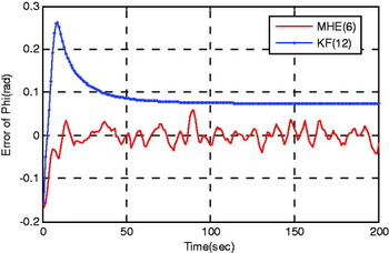
Figure 2. Estimation error of ‘Phi’.

Figure 3. Estimation error of ‘Csai’.

Figure 4. Estimation error of ‘Gamma’.

Figure 5. Estimation error of ‘ve’.

Figure 6. Estimation error of ‘vn’.

Figure 7. Estimation error of ‘vu’.

4.2. Scenario 2: ‘Zero- Manoeuvre Motion’

Here the vehicle manoeuvre is taken into consideration, and the consequent estimations of misaligned states are depicted in Figures 8–13.

Figure 8. Estimation error of ‘Phi’.

Figure 9. Estimation error of ‘Csai’.

Figure 10. Estimation error of ‘Gamma’.

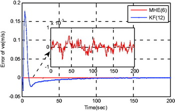
Figure 11. Estimation error of ‘ve’.

Figure 12. Estimation error of ‘vn’.

Figure 13. Estimation error of ‘vu’.

As depicted in Figures 2–7, in traditional TA framework, if the uniform turn manoeuvre is available, the initial misalignment will converge to less than 0·05 rad and 0·001 (m/s) in nearly 50 seconds, respectively. While in the zero-manoeuvre motion case that as depicted in Figures 8–13, the estimation errors are nearly 0·1 rad and 0·001 (m/s) after 100 s. These results correspond with the fact that the weak observability of instrumental errors will indirectly decrease the evaluating accuracy of attitude and velocity states along with the coupled relationships among them (Rogers, Reference Rogers2002). Meanwhile, provided the proposed CTA framework is adopted, the initial misalignment on attitude and velocity states can approximately convergent to less than 0·01 rad and 0·001 (m/s) respectively in 10 s (the horizon window length of MHE).