


1. INTRODUCTION
A navigational line of position (LOP) is a line on the surface of the Earth that represents the locus of possible positions of an observer at a given time, obtained from some type of observation. As described in Bowditch (DMA, 1977), ‘a line of position may be a straight line (actually a part of a great circle), an arc of a circle, or part of some other curve such as a hyperbola’. If the observer's position is approximately known at the time of the observation, an LOP can usually be represented as a straight line in the vicinity of the approximate position, within the area of uncertainty. A positional fix is defined by the intersection of two or more LOPs, and linearising the geometry simplifies the fix determination, whether by hand plotting or calculation. In this paper, we assume that the error in the estimated position of the observer is sufficiently small that plane geometry can be used within the area of interest near that position (i.e. a flat-Earth approximation) and that all LOPs, regardless of their source, are straight lines within this area.
If a moving observer obtains LOPs at different times, determining a fix from them requires that the LOPs be transferred to a common time. The procedures for advancing or retiring LOPs (for a ‘running fix’) are described in all navigational texts, and in this paper it is assumed that such a procedure has been performed, yielding a set of LOPs that apply to a single reference time, which serves to correct the estimated position of the observer at that time.
The effect of errors in LOPs on the computed position of an observer is dealt with in great detail in Vol. III of the Admiralty Manual (Admiralty, 1970), with particular emphasis on systematic errors. In this paper, however, the discussion is limited to random errors, which are the subject of statistical analysis. Because every LOP results from an observation with some associated uncertainty (random error), an LOP can be thought of as a fuzzy line or a ridge of high probability but finite width (Anderson, Reference Anderson1971); see Figure 1(a). Using the uncertainty in the position of each LOP in a set of LOPs that converge near the true position of the observer, it is straightforward to compute the 2D probability density function of the observer's position within an area of interest centred on the estimated position at the reference time. This function can be used to determine a position fix, independent of the type of observations that were used, and is also useful in evaluating the total probability that the observer's position lies within defined areas on the surface of the Earth.
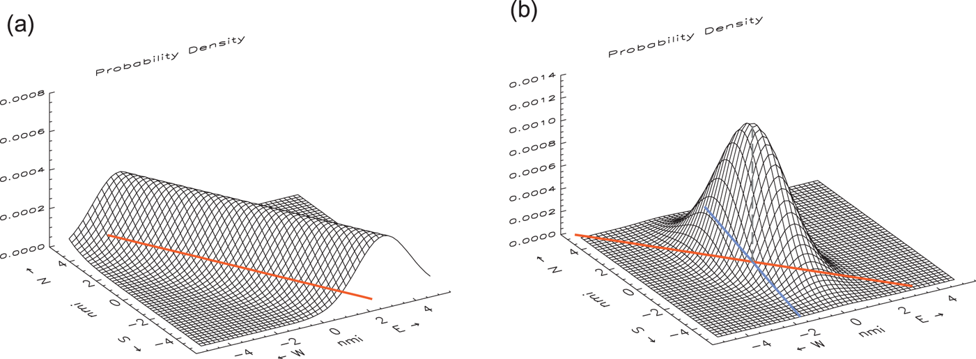
Figure 1. Plots of the probability density function for the position of the observer from (a) a single LOP, and (b) two LOPs that intersect at an angle of 50° near the centre of the x − y plane. The z-axis scale is arbitrary. The lateral uncertainty in all the LOPs is σ = 1 nmi. The function for more than two LOPs generally resembles (b).
2. COMPUTING THE 2D PROBABILITY DENSITY FUNCTION
The probability density function for an LOP that is uncertain by an amount σ, the standard deviation of the possible lateral positions of the line, is  $[ 1/( \sigma \sqrt {2\pi } ) ] \exp [ -( 1/2) ( r/\sigma ) ^{2}] $, where r is the perpendicular distance from the nominal (mean) position of the line. This expression represents a Gaussian distribution of possible parallel LOPs. The standard deviation is obtained from the uncertainty of the observation, assumed here to be unbiased. For a celestial LOP, the value of σ in nautical miles is equal to the uncertainty of the observed star altitude in arcminutes. For an LOP obtained from a bearing to a known landmark, the value of σ is the uncertainty in the coordinates of the landmark plus the uncertainty of the angular measurement (in radians) times the distance to the landmark. If the landmark is sufficiently distant, then a single value of σ will suffice in the immediate vicinity of the observer's estimated position.
The probability density function can also be thought of as being proportional to the probability that a point p that is a distance r from the LOP is actually on the LOP. Therefore, if there are N LOPs to consider, then the probability density function P at point p, representing the probability that the point is simultaneously on all of them, must be just the product of the individual probability densities:
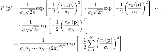 $$\begin{aligned}P\left({\bf p} \right)&=\frac{1}{\sigma _1 \sqrt {2\pi }}\hbox{exp}\left[ {-\frac{1}{2}\left( {\frac{r_1 \left( {\bf p}\right)}{\sigma _1 }} \right)^2} \right]\cdot \frac{1}{\sigma _2 \sqrt {2\pi} }\hbox{exp}\left[ {-\frac{1}{2}\left( {\frac{r_2 \left( {\bf p}\right)}{\sigma _2 }} \right)^2} \right]\cdot \cdots \\ & \quad \cdot \frac{1}{\sigma _N \sqrt {2\pi } }\hbox{exp}\left[{-\frac{1}{2}\left( {\frac{r_N \left( {\bf p} \right)}{\sigma _N }}\right)^2} \right] \\ &=\frac{1}{\sigma _1 \sigma _2 \cdots \sigma _N \cdot \left( {2\pi }\right)^{N/2}}\mbox{exp}\left[ {-\frac{1}{2}\sum\limits_{i=1}^N {\left({\frac{r_i \left( {\bf p} \right)}{\sigma _i }} \right)^2} } \right]\end{aligned}
$$
$$\begin{aligned}P\left({\bf p} \right)&=\frac{1}{\sigma _1 \sqrt {2\pi }}\hbox{exp}\left[ {-\frac{1}{2}\left( {\frac{r_1 \left( {\bf p}\right)}{\sigma _1 }} \right)^2} \right]\cdot \frac{1}{\sigma _2 \sqrt {2\pi} }\hbox{exp}\left[ {-\frac{1}{2}\left( {\frac{r_2 \left( {\bf p}\right)}{\sigma _2 }} \right)^2} \right]\cdot \cdots \\ & \quad \cdot \frac{1}{\sigma _N \sqrt {2\pi } }\hbox{exp}\left[{-\frac{1}{2}\left( {\frac{r_N \left( {\bf p} \right)}{\sigma _N }}\right)^2} \right] \\ &=\frac{1}{\sigma _1 \sigma _2 \cdots \sigma _N \cdot \left( {2\pi }\right)^{N/2}}\mbox{exp}\left[ {-\frac{1}{2}\sum\limits_{i=1}^N {\left({\frac{r_i \left( {\bf p} \right)}{\sigma _i }} \right)^2} } \right]\end{aligned}
$$where r i(p) is the distance of point p from LOPi, which has an uncertainty in position characterised by a standard deviation σi. In some cases, for example, celestial observations, all of the σi values will be the same, or nearly so.
If we establish a Cartesian coordinate grid with the origin at the estimated position of the observer, with x positive to the east and y positive to the north, then the point p has coordinates (x,y) and Equation (1) can be re-expressed as:
 $$P( {x,y} ) =\alpha\ \hbox{exp}\left[ {-\frac{1}{2}\sum_{i=1}^n {\left( {\frac{r_i ( {x,y} ) }{\sigma_i }} \right)^2} } \right]$$
where r i(x,y) is the perpendicular distance between the point at coordinates (x,y) and LOPi. Expressions for r i(x,y), which depend on how the LOPs are represented mathematically, are given in Supplementary Appendix A (Kaplan, Reference Kaplan2018). For Equations (1) or (2) to represent meaningful probabilities, they must be normalised and then evaluated over some finite area of the Earth's surface. The factor α in Equation (2) represents the normalisation described in the following paragraph, so that the initial factor in Equation (1), involving the product of all the σi values, is not important. Equation (2) forms the basis of the method of least squares (to determine, in this case, the coordinates of the fix), derived from the principle of maximum likelihood (Young, Reference Young1962; Bevington and Robinson, Reference Bevington and Robinson2003; or other elementary statistical texts).
We can therefore apply Equation (2), initially with α = 1, to a grid of points centred near the observer's estimated position. The grid should extend outwards to points that have, a priori, zero or near-zero probability of being the actual position of the observer. Then, normalising the probabilities consists merely of adding up all the values computed from Equation (2) for the entire grid, then dividing each value by the sum. The sum of all the resulting probability values is then 1, as it must since, by construction, the grid of points must cover all possible positions of the observer. Practically, this means that the grid must extend outwards from its origin to at least to four or five times the standard error of the estimated position of the observer, assuming the standard errors of the LOPs are no worse – that is, assuming that they converge within a small area near the origin. For the results presented in this paper, a 101 × 101 grid was used (10,201 points total), with the scale inversely proportional to the greatest value of σi used in Equation (2). The centre was set near the point of maximum probability, which is the same as a least-squares fix obtained from the same observations. In this way, a probability map for the actual position of the observer can be computed.
The probability calculation can also include LOPs that are circular arcs, for example, those from range (distance) measurements, or from celestial observations of objects near the zenith – see Section 6 below.
3. APPLICATIONS
The probability density function, evaluated for a grid of discrete points as described in the previous section, provides a nontraditional approach to determining a navigational fix and understanding its reliability. A plot of this function for two intersecting LOPs of equal uncertainty is shown in Figure 1(b). The position fix is at the high point of the broad hill of increased probability, at the point at which the two LOPs intersect. More generally, regardless of the number of LOPs involved, the probability maximum is coincident with the fix, as determined by other common methods (unbiased maximum-likelihood estimators). Contour lines of equal probability are ellipses centred on the fix position; all such contours have the same shape and orientation.
The scheme described in Section 2 generally has no advantage over (and is computationally more laborious than) commonly used analytical approaches if all one is interested in is the fix position, its uncertainty, and the equal-probability contours. Standard least-squares software provides all the information needed. The advantage of computing the probability density function for a grid of points is that such a grid allows us to determine the total probability that the observer's position lies within some defined geographic area of interest, however irregular and wherever located. For example, it might be important to evaluate the probability that the observer is within (or outside) a zone of avoidance surrounding a known navigational hazard. Suppose it is deemed prudent to allow a separation of s miles between the observer and a charted hazard; it is easy to simply add up the probability values for grid points that satisfy the condition that (x − x h) 2 + (y − y h) 2 ≤ s, where the coordinates of the hazard are (x h, y h). Of course, for an extended hazard such as a shoal, the area to be evaluated might be larger and represented as some kind of polygon. The procedure described above might be applicable, therefore, to navigational systems that map LOPs (from whatever source) onto electronic charts that display channels, shoals, hazards, and other objects of interest. Commercial or open-source 2D integration software (e.g. Mathworks, 2019; or Press et al., Reference Press, Teukolsky, Vetterling and Flannery1993) could be employed for the computations, although accommodating irregular areas in the (x,y) plane to be integrated might be challenging.
Also, unlike a least-squares solution for the fix, which provides no error estimates for a two-LOP fix (no degrees of freedom in the problem), it is feasible to construct a probability map for such a case using Equation (2), as long as there are estimates of the uncertainties in the positions of the LOPs (σi values).
4. EXPERIMENTS
In order to assess the correctness and accuracy of this procedure, it was applied to several specific areas near a fix where the total probability is known from previous analytical developments. In the process of verifying the procedure, some interesting results were obtained that provide a useful perspective on interpreting the reliability of computed navigational fixes generally.
In these experiments, the observations defining the LOPs all have the same uncertainty, which is what is usually assumed (even if not entirely correct). The case of unequal uncertainties is covered in Supplementary Appendix B (Kaplan, Reference Kaplan2018); the results are similar to what is described below.
4.1. The ‘cocked hat’ problem
The first experiment was for a fix determined by three LOPs, where it is straightforward to compute the total probability that the observer's true position lies within the triangle formed by the near intersection of the LOPs (the computed fix will always be there). This is sometimes referred to as the ‘cocked hat’ problem, and it has been addressed previously in the literature (e.g. in this journal, see Cotter, Reference Cotter1961; Parker, Reference Parker1961; Lee, Reference Lee1991; Williams, Reference Williams1991; Gething, Reference Gething1992; Swift, Reference Swift1992; Cook, Reference Cook1993). Based on geometric arguments, a total enclosed probability of 25% for the triangle has been well established. But a geometric construction does not indicate that there is actually a spread of probability values depending on the LOP geometry, with 25% being an average.
Using the scheme described above, we are now in a position to reevaluate the LOP triangle probability based on the assumption of a Gaussian distribution of errors. Recently, Stuart (Reference Stuart2019) has given an analytical development for this case that verified the 25% average probability for triangles formed by three LOPs, based on Gaussian statistics. For the current paper, Monte Carlo-type numerical tests were conducted with the 101 × 101 grid described above, populated with normalised probability density values from Equation (2) with N = 3. For each test case, three LOPs were derived from three randomly generated synthetic observations relative to the hypothetical observer position. A test run consisted of 100 of these randomly generated tests cases.
Consider cases where the three LOPs are of equal uncertainty, σLOP, which was an input parameter for the run. In each such case, the software generated a random error in the position of each LOP (orthogonal to its direction) taken from a Gaussian distribution of possible errors with zero mean and standard deviation σLOP. The azimuths of the LOPs were also randomised. (For celestial observations, σLOP is also the standard deviation of the observations if we equate arcminutes to nautical miles.) Then, Equation (2) was evaluated for each point on the grid. For the first set of runs, the obvious choice was to set all the σi values in Equation (2) to σLOP; that is, if σ (unsubscripted) is the common uncertainty value to use in Equation (2), then σ = σLOP. For each case, i.e. each set of three LOPs, the probabilities of the points within the LOP triangle were then added up. The probability computed this way depends critically on the value of σLOP relative to the size of the triangle.
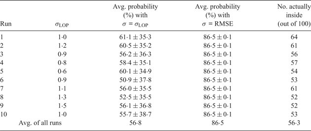
Each run of 100 cases thus yielded, for a single σLOP value, 100 computations of the probability that the observer is within the LOP triangle. The results are given in Table 1, col. 3; the computed LOP triangle probabilities are spread over a fairly wide rangeFootnote 1 but seem to be generally centred around the 25% canonical value.
Table 1. Probabilities of observer inside LOP triangle for 3 LOPs of the same uncertainty.

Each run is 100 random test cases.
However, in the real world, there may be only a rough estimate of what the value of σLOP is. We generally assess the uncertainties in the LOP positions – which might vary widely, depending on the conditions under which the observations were taken – as part of the fix determination. The degree of convergence of the LOPs is taken as an indication of the quality of the observations. Quantitatively, a least-squares (or equivalent) solution for the fix yields a value for the root-mean-square-error (RMSE) of the fit (square-root of the variance), a measure of the distances of the three LOPs from the fix location, (x f,y f). Unlike σLOP, the RMSE is a computed quantity that varies from case to case. For each case, the RMSE value can be obtained without a least-squares solution for the fix by using instead the point of maximum probability, as computed from Equation (2), as the fix location.
Therefore, in a second set of test runs, there was no presumed knowledge of σLOP for the Equation (2) evaluation – even though the software uses a specific value of σLOP to generate errors in the LOP positions – and σ in Equation (2) was set to the computed RMSE value from the fix determination. That is, these runs use an a posteriori estimate of the uncertainty in the lateral positions of the LOPs to set the value of σ in Equation (2). The result of these test runs was surprisingly consistent: the probability of the true position lying inside the ‘cocked hat’ triangle was almost always computed to be about 33·5%. Clearly using σ = RMSE yields a different result than using σ = σLOP. The case-by-case variation in these probabilities is small because, for each case, the RMSE value essentially scales itself to the size of the triangle.
Because each test case is a computational model, the true (hypothetical) position of the observer is known. Therefore, the software can determine whether the observer's position is actually within the LOP triangle for each case. For each run of 100 cases, the software counts the number of observer positions inside the triangles, and that statistic is listed in Table 1, col. 5. These numbers, considered as a percentage, are comparable to those listed in col. 3, and are consistent with the expected 25% probability.
The probabilities computed using σ = RMSE shown in col. 4 are clearly more optimistic than are those shown in cols. 3 and 5. The reason is that, although there is a wide variation in the RMSE values, taken as a whole they tend to be less than σLOP (i.e. the RMSE understates the standard deviation of the parent distribution of errors for these experiments). In the computer runs that are the basis for Table 1, the average of all the RMSE values is smaller than σLOP by about 19%. Therefore, when the RMSE values are used in Equation (2), the resulting probabilities are greater, overestimating the actual probabilities. A discussion of why this occurs and its implications for navigation software is presented in Section 7.
If the observations defining the LOPs have different uncertainties, which might be the case if the observations are of different types, then the situation is a bit more complicated mathematically, but analogous. The results are similar to those described above and are presented in Supplementary Appendix B (Kaplan, Reference Kaplan2018). It is also shown there that setting σ = RMSE, as described, is equivalent to requiring that the reduced chi-squared (chi-squared value per degree of freedom),  $\chi_{\nu}^{2}$, for the fix solution is equal to 1, which is the ideal case, statistically.
4.2. Error ellipses
A least-squares solution for a fix provides a 2 × 2 variance-covariance matrix for the solved-for parameters (x f and y f), which can be used to define error ellipses of various sizes, centred on the fix position. Each such ellipse encloses a known total probability that the observer's actual position lies within it (see developments in, e.g. Bowditch (DMA, 1977), Bomford (Reference Bomford1980), or Trumpler and Weaver (Reference Trumpler and Weaver1953)). The size and total probability enclosed by an error ellipse are determined by its size factor S, where an S = 1 ellipse encloses a total probability of 39%, an S = 2 ellipse (twice the linear size) encloses 86%, and more generally, the enclosed probability P e = 1 − exp( − S 2/2). An error ellipse with enclosed probability P e is coincident with the probability contour (relative to the maximum probability) at 1 − P e.
The computer runs that were used to populate Table 1 were modified to evaluate, for each case, the probability interior to an S = 2 error ellipse instead of the LOP triangle. The results are given in Table 2, which has been constructed in a manner completely analogous to that used for Table 1. The values in col. 4 show that when the RMSE value is used in Equation (2) – that is, when it is assumed that RMSE indicates the width of the parent distribution of errors – the theoretical probability for the ellipse is consistently obtained. However, just as in Table 1, the values in cols. 3 and 5 tell a different story. The values in col. 5 simply report on the geometric results and are not dependent on any statistical theory. The values in col. 3 come from Equation (2) based on σ = σLOP, which is the actual width of the parent distribution of errors. Cols. 3 and 5 are consistent, and indicate that the actual average probability of the observer being in the S = 2 error ellipse, for a three-LOP fix, is about 56%, not 86%. This result also holds if the three observations for each case have different uncertainties. See the discussion of this discrepancy in Section 7.
Table 2. Probabilities of observer inside S = 2 error ellipse for 3 LOPs of the same uncertainty.
Each run is 100 random test cases.
4.3. LOP polygons
A formula developed by Daniels (Reference Daniels1951) provides an interesting – although apparently not well known – generalisation of the three-LOP case. Daniels obtained a formula for the probability enclosed by the largest polygon formed from any number of convergent LOPs: P N = 1 − N/(2N−1). Therefore, we have P N = 0 · 2500, 0·5000, and 0·6875 exactly for N = 3, 4, and 5 LOPs, respectively. It was not difficult to generalise the software used for the LOP triangle tests described above to evaluate the probabilities interior to LOP polygons, since polygons can be decomposed into triangles. Four- and five-LOP geometries were evaluated, with σ = σLOP, based on 2500 random cases each. The results were, for four LOPs, an average interior probability of 49·9%, with 49·4% of the observer positions actually inside the quadrilaterals; and for five LOPs, an average interior probability of 68·1%, with 67·5% of observer positions actually inside the pentagons. Considering that the RMS spread in the computed probability values exceeds 20% (but see footnote 1), the procedure in this paper provides results reasonably consistent with Daniels's formula for these cases.
5. CHECKS ON THE PROCEDURE
A least-squares solution for the fix position based on three or more LOPs provides an independent check on the probability calculations described before. (The algorithms are independent, although the basis in statistical theory is the same.) The coordinates of the fix obtained from such a solution, (x f,y f), can be compared to the coordinates of the point of maximum probability, (x max,y max), within the map of probability values constructed from Equation (2). Although the map has probability values only at discrete points, applying Newton's method to find the zeros of the probability gradient components ∂ P(x,y)/∂ x and ∂ P(x,y)/∂ y at (x max,y max) provides a more precise estimate of the coordinates of the actual probability maximum. (Other methods of numerically solving for the maximum probability can, of course, be used. Taking the natural log of the probability values results in gradient components that are linear in the coordinates.) Such a procedure yields probability maxima that match the least-squares fixes to within about 1/10 of the grid spacing in the map, which is a small fraction of the formal errors of the fix coordinates. Note that this is just a brute-force application of the principle of maximum likelihood.
The numerical experiments described in the Section 4 also showed that the total probabilities computed within the triangles and polygons were consistent with what is expected from independent developments, when σ = σLOP, i.e. the actual width of the parent distribution of errors was used in Equation (2). Furthermore, the probability sums were consistent with the number of hypothetical observers actually found within the figures (considering the latter as ‘truth’ data).
The experiments with error ellipses showed that the ellipses overlay the probability map computed from Equation (2) at contour 1 − P e (with P e defined in 4.2), as expected, for cases with three or more LOPs where the  $\chi_{\nu}^{2}=1$ condition is imposed. That condition applies to LOPs with the same uncertainty σ = RMSE; or, for LOPs with different uncertainties, where the individual σi values are normalised as described in Supplementary Appendix B (Kaplan, Reference Kaplan2018). In all these cases, the RMS difference between the ellipse probability from the map summation and P e was only about 0·1% for ellipses of several sizes. Figure 2 shows a typical rendition of an S = 1·55 error ellipse, with enclosed probability 70% (0·7), that coincides with the 0·3 probability contour on the map. Note that these tests only confirm the consistency between the two methods of computing probability when $\chi_{\nu }^{2}=1$ and do not necessarily reflect real-world accuracy.
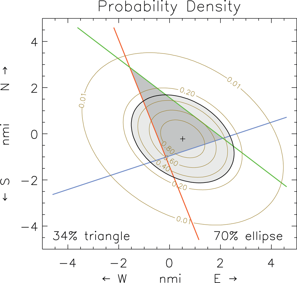
Figure 2. A probability map from three LOPs, in a  $\chi _{\nu}^{2}=1$ case (σ = RMSE), showing contours of constant probability and, superimposed, an error ellipse (in light grey) from a least-square solution.
The software used for the LOP triangle (‘cocked hat’) tests described in Section 4.1 was also successfully tested against independent developments by Stuart (Reference Stuart2018, Reference Stuart2019), some of which are based on analytical formulas for probabilities that have been computed numerically here.
Therefore, the available evidence indicates that the procedure outlined in this paper, based on Equation (2), produces realistic probability values, given the geometric and statistical models used.
6. EXTENSIONS
Circles of position from either a measurement of the distance to a known landmark or a celestial observation of a star near the zenith can also be incorporated into Equation (2). In both cases, the coordinates of the centre of the circle are known. In the first case, it is the latitude and longitude of the landmark and in the second case, it is the Greenwich Hour Angle and Declination (GHA and Dec in the almanacs) of the star observed, which define the geographic position (GP) where the star is at its zenith. The distance D of either of these points from points in the probability map can therefore be computed from the usual spherical trigonometry formulas, given the association of any point (x,y) on the map with a latitude and longitude. The distance of the circle of position from a point on the map is then simply r j(x, y) = |d − D|, where d is the measured distance. In the celestial case, d = 90° − Ho, where Ho is the observed altitude of the star (adjusted for all the usual corrections to a sextant altitude). Conversion between angular and linear units is required at some point.Footnote 2 For a very distant terrestrial landmark, or where the measurement of its distance d is very precise, the spherical-trigonometry formula for D should be replaced by a geodesic formula (Karney, Reference Karney2013, for example). A further complication is that transferring circles of position to account for the motion of the observer is not as simple as transferring lines of position; Kaplan (Reference Kaplan1996) treats the celestial case.
The estimated position of the observer could be factored into the probability map, as a term in Equation (2), if its radial uncertainty, σEP (characterising a circular normal distribution), can be realistically assessed. Note that the estimated position is a point, not a line, so the probability distribution is radial (2D), not lateral (1D), with a different integrated probability as a function of distance. The probability density function for a circular normal distribution, with centre at (x EP,y EP) and radial uncertainty σEP, is the same as for two orthogonal ‘virtual’ LOPs, each with lateral uncertainty σEP, that intersect at (x EP,y EP). The addition of the estimated position to the probability map increases the value of N characterising the map by 2.
Conceptually, Equation (2) could be used for 3D problems if r j(x,y) is replaced by r j(x,y,z). Lines and circles of position on the surface of the Earth are replaced by lines, planes, and spheres in space, depending on the type of observation, and the probability map P(x,y) becomes a probability ‘cloud’ P(x,y,z). (For least-square solutions, the error ellipse becomes an error ellipsoid.) The formulas for r j(x,y,z) are fairly simple if expressed in vector notation for a 3D rectangular coordinate system (Hummel, Reference Hummel1965).
Equations (1) and (2) could be reformulated to use, as a basis, error distributions that are symmetric about each LOP but not Gaussian, although such a reformulation would then have no relationship to the least-squares solutions for the same problems.
7. USING LARGE-N STATISTICAL METHODS FOR SMALL-N CASES
In the numerical experiments described in Section 4.1 (the ‘cocked hat’ runs), the ensemble of RMSE values computed from post-fit residuals was described as being systematically less than σLOP, which is, by construction, the standard deviation of the parent distribution of LOP errors. (The RMS width of the actual distribution of LOP errors used in each run closely matched the input σLOP value.) Using σ = RMSE in Equation (2) therefore results in higher probabilities than are realistic.
Why are the RMSE values, on average, less than σLOP? In each case considered, the observational errors randomly generated for the three LOPs do not by themselves well represent the parent distribution of errors. Usually, the three errors generated are asymmetric with respect to the parent distribution. But because the RMSE is measured with respect to the fix position, which reflects a kind of 2D average of those errors, the RMSE value will in most cases be less than σLOP – the least-square fix position minimises the RMSE value. The same tendency can be seen in 1D cases with three random samples of an uncertain quantity, drawn from a known distribution. In sampling theory, this is referred to as a ‘biased estimate of the standard deviation’. Holtzman (Reference Holtzman1950), Cureton (Reference Cureton1968), and other references, including a Wikipedia entry (2019), provide correction factors for the measured standard deviation – applied to make it an unbiased estimate of the standard deviation of the parent distribution – when the number of samples (observations) is small. The corrections are rather modest (for N = 3, the factor is 1·13) but they apply only to 1D problems.
Furthermore, because small errors in the LOPs are more probable than are large ones, it turns out that many of the LOP triangles randomly created are smaller than what we might naively expect; the distribution of triangle areas ramps up steeply towards the small end. The probability that the observer is in one of these small triangles is low. Triangles with enclosed probabilities <10% accounted for 30–40% of all triangles generated by the software. It is unsurprising, then, that, considering all possible cases, the probability that the observer's position is actually within the triangle is only, on average, 25%. However, in each case, the RMSE value adjusts itself to the size of the triangle (while σLOP remains a constant for all cases), yielding the 33·5% probability shown in Table 1, col. 4, independent of the size of the triangle.
The fact that the RMSE value tends to underestimate σLOP has implications for commonly used navigation software – or, at least, for the interpretation of the output. Software that computes a least-square fix position also usually displays a graphic showing the LOPs, the estimated (or DR) and fix positions, and an error ellipse (as described in Section 4.2) centred on the fix. For example, the NavPac celestial navigation software (HMNAO, 2015), developed by H.M. Nautical Almanac Office and used by the Royal Navy, displays such a graphic, as does software used by the U.S. Navy and Coast Guard. The NavPac ellipse is drawn to include the actual position of the observer 95% of the time, according to statistical theory. The U.S. Navy software displays an S = 2 ellipse which, in theory, includes the actual position of the observer 86·48% of the time. These statistical estimates are stated in the user guides. However, the theory is based on perfect knowledge of the parent distribution of errors, which the software does not have. These ellipses are based on RMSE (or some related measure) which, for N = 3, tends to underestimate the width of that distribution. In celestial navigation, three-body fixes are common, and in these cases, the stated probabilities that the observer is within the error ellipse are too optimistic. How optimistic?
Table 2, computed for three-LOP error ellipses, provides a partial answer. There, the probability values in col. 3, based on σ = σLOP, which is the actual width of the parent distribution of errors, are significantly less than those in col. 4, based on σ = RMSE. The values in col. 5, which are a simple count of hypothetical observers found within the ellipse, are consistent with the lower probabilities shown in col. 3. Table 2 has been computed for an S = 2 error ellipse but a set of similar runs shows that a 95% (S = 2·45) error ellipse actually encloses a 64% probability when σ = σLOP. Thus, in the common case of three LOPs, the theoretical probabilities associated with error ellipses are not appropriate, and software users should not assume that those probabilities reflect the actual uncertainties.
We expect RMSE → σLOP as N → ∞. In fact, that is what we find experimentally as the number of LOPs increases. For the runs that contributed to Table 2, the ratio of the average RMSE value to σLOP is 0·81. For those same runs but with four LOPs, the ratio is 0·87; with six LOPs, 0·95; and for ten LOPs, 0·97. If\ Table 2 were reconstructed for each of these additional sets of runs, the bottom-line averages for cols. 3 and 5 (the col. 4 values do not change) would be, for four LOPs, 65·7 and 64·4, respectively; for six LOPs, 75·5 and 76·9; and for ten LOPs, 80·6 and 79·0. This shows that the error-ellipse probabilities from statistical theory do become increasingly realistic (‘reality’ being defined here as these numerical tests) as N increases, but their use for small-N cases, as is common, clearly presents an over-optimistic picture.
A related piece of information to come out of these simulations is that for the three-LOP cases, the value of σLOP for a given case is a much more reliable predictor of the actual radial error of the fix than is RMSE, which in a significant number of cases (presumably the small triangles of low interior probability) seriously underestimates the radial error.
8. CONCLUSION
A simple procedure has been presented, based on Equation (2), for constructing a probability map for the position of an observer, given two or more lines of position obtained from observations. The equation is based on LOPs that have been advanced or retired to refer to a common time, with Gaussian-distributed lateral errors. The characteristics of each resulting map are consistent with those predicted by an independent least-square solution for the navigational fix based on the same LOPs. The map allows for considerable flexibility in assessing the probability that the observer is within (or outside) areas of interest on the surface of the Earth, however irregular, such as hazard zones. Such an assessment has been presented for problems involving three LOPs, where the probability that the observer is within the triangle formed by the converging LOPs has been shown to average about 25%, consistent with previous estimates. The probability map procedure has been used to explore the relationship between theoretically derived probabilities for standard navigational error ellipses and those likely to be encountered in practice. It was found that the theoretical probabilities approach realistic probabilities for fix solutions involving many observations but are significantly too optimistic for cases where only a few observations are available. The procedure can be easily modified to incorporate positional information other than that from straight-line LOPs, and can be generalised to navigational problems in three dimensions.
SUPPLEMENTARY MATERIAL
The supplementary material for this article can be found at https://doi.org/10.1017/S0373463319000912.
ACKNOWLEDGEMENTS
I thank Robin Stuart for very useful discussions and software comparisons. This work was supported by the U.S. Navy (contracts N0018915PZ329 and N0018918PZ403).


 Open access