


Introduction
Only about 1% of the global glacier population has been inferred to be of surge type (Reference Jiskoot, Boyle and MurrayJiskoot and others, 1998). Nevertheless, studies of surge-type glaciers have an invaluable impact on our understanding of ice-flow instabilities and fast glacier flow (e.g. Reference BuddBudd, 1975; Reference KambKamb and others, 1985; Reference FowlerFowler, 1989). One of the distinctive characteristics of surge-type glaciers is their geographical distribution. Clusters of surge-type glaciers are observed in specific glaciated regions, and even within cluster regions surge-type glaciers are not uniformly distributed (Reference PostPost, 1969; Reference Clarke, Schmok, Ommanney and CollinsClarke and others, 1986).
There has been a suite of studies assessing the environmental controls on surging and fast flow. These studies cover glacier populations of western North America; the Yukon Territory, Canada; Central Asia; and Svalbard. Some of these studies used qualitative observations (Reference PostPost, 1969), others univariate statistical analysis (Reference GlazyrinGlazyrin, 1978; Reference Clarke, Schmok, Ommanney and CollinsClarke and others, 1986; Reference WilburWilbur, 1988; Reference HamiltonHamilton, 1992; Reference Hamilton and DowdeswellHamilton and Dowdeswell, 1996) and multivariate statistical analysis (Reference ClarkeClarke, 1991; Reference Marshall, Clarke, Dyke and FisherMarshall and others, 1996; Reference Atkinson, Jiskoot, Massari and MurrayAtkinson and others, 1998; Reference Jiskoot, Boyle and MurrayJiskoot and others, 1998).
One prominent cluster region of surge-type glaciers is Svalbard. We estimate the percentage of surge-type glaciers in this region to be about 13% (Reference Jiskoot, Boyle and MurrayJiskoot and others, 1998), although others put the value at 90% (Reference Lefauconnier and HagenLefauconnier and Hagen, 1991). The spatial distribution of surge-type glaciers within regions like Svalbard is thought to be a function of the distribution of glaciers with distinctive attributes (Reference Hamilton and DowdeswellHamilton and Dowdeswell, 1996). Recently a multivariate logit analysis was used to distinguish between surge-type and normal glaciers in Svalbard (Reference Jiskoot, Boyle and MurrayJiskoot and others, 1998). The analysis indicated that long glaciers with relatively steep slopes overlying young fine-grained sedimentary lithologies, with orientations in the arc northwest to southeast, are most likely to be of surge-type. Likewise, from most other studies glacier length and specific substrate conditions emerge as factors of greatest association to the distribution of surge-type glaciers (Reference GlazyrinGlazyrin, 1978; Reference ClarkeClarke, 1991; Reference Hamilton and DowdeswellHamilton and Dowdeswell, 1996; Reference Atkinson, Jiskoot, Massari and MurrayAtkinson and others, 1998) and as controls of fast-flowing ice streams (Reference Marshall, Clarke, Dyke and FisherMarshall and others, 1996). However, none of the variables satisfactorily explains the distribution of surge-type glaciers or reveals explicit controls on surging. This raises the issue of whether the correct variables are being analyzed. Glacier length could be a proxy for other factors such as mass balance (Reference BuddBudd, 1975), hypsometry (Reference GlazyrinGlazyrin, 1978; Reference WilburWilbur, 1988), subglacial conditions (Reference PostPost, 1969; Reference ClarkeClarke, 1991) or thermal conditions (Reference ClarkeClarke, 1976; Reference Kotlyakov and MacheretKotlyakov and Macheret, 1987). Consequently, this paper extends the analysis presented in Reference Jiskoot, Boyle and MurrayJiskoot and others (1998) to include geological boundaries, mass-balance proxies in the form of accumulation-area ratio (AAR) and glacier hypsometry measures, and a measure of thermal regime. We examine the possible influence of each of these factors on the likelihood of surging for glaciers in Svalbard using a multivariate logit regression model. We then extend this analysis to examine the residuals, which allows us to identify glaciers that have not been classified as surge-type before but that have characteristics of surging glaciers, and vice versa.
Data Description
Reference Hagen, Liestøl, Roland and JørgensenHagen and others (1993) compiled a detailed glacier inventory of 1029 glaciers larger than 1 km2 in the High Arctic archipelago of Svalbard (76–81° N, 9–33° E). A complete set of data on geometry, orientation, elevation, glacier type, frontal characteristics and activity was available for 504 of the 1029 glaciers. These tended to be the larger glaciers covering about 93% of the total glaciated area of Svalbard (see Fig. 1). We classified this set of 504 glaciers as surge-type, and normal glaciers on the basis of the previous literature (e.g. Reference Lefauconnier and HagenLefauconnier and Hagen, 1991; Reference LiestølLiestøl, 1993). Additionally, air-photo interpretation was used to collect primary surge evidence for those cases where the documentation on a glacier surge was ambiguous, or where glaciers were listed as surge-type on the basis of disputable morphological evidence for surging (e.g. Reference Croot and CrootCroot, 1988). Most Svalbard glaciers are covered by at least three stereo-sets of Norsk Polarinstitutt air photos covering the period 1936–95.

Fig. 1. Distribution of 50 glaciers with a continuous internal reflection horizon (IRH) in dark shading and 87 glaciers without IRH in grey shading These RES-surveyed glaciers delineate, together with the light-shaded unsurveyed glaciers, the location of the 504 Svalbard glaciers used in this research. Primary RES data sources are Reference Macheret and ZhuravlevMacheret and Zhuravlev (1982), Reference Dowdeswell, Drewry, Liestøl and OrheimDowdeswell and others (1984), Reference BamberBamber (1987a, Reference Bamberb, Reference Bamber1989), Reference Kotlyakov and MacheretKotlyakov and Macheret (1987) and Reference Macheret, Kotlyakov and SokolovMacheret (1990).
Various morphological criteria can be used to distinguish surge-type glaciers from normal glaciers (e.g. Reference Meier and PostMeier and Post, 1969; Reference Clarke, Schmok, Ommanney and CollinsClarke and others, 1986). While some features are diagnostic for surging, others are less explicit and must be studied in the context of the surge evolution. Consequently there will always remain uncertainties in the identification and classification of surge-type glaciers. It is therefore normal practice in the statistical analysis of surge-type glaciers to assign a surge index (S), representing the likelihood that a particular glacier is of surge type (Reference Clarke, Schmok, Ommanney and CollinsClarke and others, 1986). A surge index is based on the strength of evidence for surge behaviour, ranging from ambiguous morphological evidence to an observed surge. The most appropriate surge index for our logit models is a dichotomous index with S = 0 for normal glaciers (without convincing surge evidence) and S = 1 for surge-type glaciers.
We classified 132 of the 504 glaciers in our dataset as “surge-type” and 372 as “normal”. The surge-type glaciers cover about 50% of the total glaciated area in Svalbard. For all glaciers a set of 27 glacial and environmental variables were tested against the likelihood of surging (Table 1). Primary data were selected from the glacier inventory (Reference Hagen, Liestøl, Roland and JørgensenHagen and others, 1993). Secondary data were directly calculated from the primary data. Geological data were collected using Norsk Polarinstitutt geology maps and publications. Datasets on internal reflection horizons (IRHs) and thermal properties were compiled from publications only (Fig. 1). In general, the timing and accuracy of data measurements can affect our data analysis. As most of the glacier data were collected during the late 1980s (Reference Hagen, Liestøl, Roland and JørgensenHagen and others, 1993) the data used in our analysis correspond to glaciers in different stages in their surge cycle.
Table 1. Variables used in the logit data analysis

Generalized Linear Modelling: Theory of Logit Regression
For our data analysis we used logit regression models, fitted as generalized linear models (GLMs). Logit models allow us to relate a binary response variable (e.g. surge-type vs normal glaciers) to a variety of explanatory variables and their interaction terms. Further, the technique can be used both as an exploratory and as a predictive technique by focusing on the residuals calculated for each individual glacier. Theoretical descriptions of the logit method are given in Reference WrigleyWrigley (1985) and Reference Aitkin, Anderson, Grancis and HindeAitkin and others (1989). For a detailed methodology description with application to glacier surging see Reference Atkinson, Jiskoot, Massari and MurrayAtkinson and others (1998).
The logit technique models the log-odds of an event occurring in a population, based on a number of explanatory variables. The event is defined by a binary response variable: S = 1 for “presence” and S = 0 for “absence” of a surge-type glacier. The explanatory variables are the set of selected glacial and environmental characteristics (Table 1). Thus,

which is the log-odds of the probability (Pi ) that a glacier is of surge type. The logit link function f (Xi ) can be expressed as the linear predictor function or “logistic regression function”:

where α is the “base estimate”, βk are the n “estimates” or coefficients to be calculated in the model and Xik are the n values for each of the explanatory variables. The model is not linear, but has a logistic curve (an S-shaped cumulative probability distribution) and is strictly bounded such that if Xik = =−∞, then logit (Pi ) = 0 and if Xik = −∞, then logit (Pi ) = 1 (Reference WrigleyWrigley, 1985).
Model fitting, model significance and significance terms
A multivariate logit model can be fitted in a step-wise manner (see Reference Atkinson, Jiskoot, Massari and MurrayAtkinson and others, 1998). The null model only includes an intercept effect, effectively treating the estimated value for each case as average for the whole dataset. The deviance D that results in this model is a baseline against which the improvement of the model fit can be determined for the addition of each explanatory variable that corresponds with the loss of degrees of freedom through the addition of the variable. D is expressed as:
where Λc is the maximum likelihood of the current model and Λf is the maximum likelihood of the full model, which includes all variables (Reference WrigleyWrigley, 1985).
Since the deviance reduction between separate models can be approximated to have a chi-squared distribution, it can be used as an indicator of the significance of each term added to the model (Reference WrigleyWrigley, 1985). Only those variables that are significant at a given confidence level are retained. In all our models a confidence level of 95% was used. The significance of the estimated coefficients β in Equation (2) can be tested using the Student t test, where the t value is calculated by dividing the estimated coefficient by its standard error. For a large sample size (over 120) the critical Student t value at the 95% significance level is 1.96. A coefficient is therefore significant when it is greater than approximately twice the standard error (Reference WrigleyWrigley, 1985). Positive coefficients indicate a direct relationship between the variable and surge-type glaciers, and negative coefficients an inverse relationship. The larger the estimated coefficient, the stronger the correlation.
Logit analysis is usually performed in two stages: (1) a univariate stage, where the relationship between each variable and the incidence of surging is examined individually (see Reference Jiskoot, Boyle and MurrayJiskoot and others, 1998), and (2) a step-wise multivariate stage, where the combined effects of variables on glacier surging are examined simultaneously. At each step in the multivariate stage the interaction terms (the product of the two main terms) between the variables can be explored and, if found to be significant, added to the model. Eventually, the optimal model is reached, in which the combination of variables is inferred to optimally discriminate between surge-type and normal glaciers.
In some cases (where non-linear relationships are expected) transformation of a continuous variable causes a much larger reduction in model deviance than the non-transformed variable and can consequently improve the model significantly. Further, fully subdivided categorical variables can contain too few observations per category and therefore give large standard errors as compared to their parameter estimates (Reference WrigleyWrigley, 1985). To resolve this problem we aggregated the classes of these variables into larger, fewer groups. Variables for which aggregated categories give better model fits are indicated in Table 1.
Residual analysis
Once an optimal logit model is reached, fitted values
![]() for each individual glacier can be compared with observed values (S) for the dependent variable. Instead of using raw residuals
for each individual glacier can be compared with observed values (S) for the dependent variable. Instead of using raw residuals
![]() , which are statistically incomparable, the GLM uses modified Pearson residuals that are standardized to have a mean of zero and a unit variance (Reference WrigleyWrigley, 1985). For our logit models the standardized residuals ei
for each glacier are calculated as:
, which are statistically incomparable, the GLM uses modified Pearson residuals that are standardized to have a mean of zero and a unit variance (Reference WrigleyWrigley, 1985). For our logit models the standardized residuals ei
for each glacier are calculated as:

where S is the assigned binary surge index and
![]() is the fitted value in the model. Large residuals indicate failure of the model to fit well for the corresponding glacier. A perfect model would give fitted values close to one for all surge-type glaciers, and fitted values close to zero for all normal glaciers. Logit models intrinsically produce a systematic pattern in the distribution of residuals (Reference WrigleyWrigley, 1985). Large residuals are generally found in the low and high fitted values; this is inherent in the dichotomous nature of the logit regression (Reference Aitkin, Anderson, Grancis and HindeAitkin and others, 1989). Statistical residual analysis techniques for least-squares regression thus cannot be applied in logit models, and residual analysis is mainly through visual interpretation of residual plots.
is the fitted value in the model. Large residuals indicate failure of the model to fit well for the corresponding glacier. A perfect model would give fitted values close to one for all surge-type glaciers, and fitted values close to zero for all normal glaciers. Logit models intrinsically produce a systematic pattern in the distribution of residuals (Reference WrigleyWrigley, 1985). Large residuals are generally found in the low and high fitted values; this is inherent in the dichotomous nature of the logit regression (Reference Aitkin, Anderson, Grancis and HindeAitkin and others, 1989). Statistical residual analysis techniques for least-squares regression thus cannot be applied in logit models, and residual analysis is mainly through visual interpretation of residual plots.
There are two causes of large residuals: (1) mis-specification of observed values for the response variable to units (glaciers) in the population, and (2) the occurrence of aberrant observations, distorting either the probability distribution or the parameter estimates for the model (Reference Aitkin, Anderson, Grancis and HindeAitkin and others, 1989). Hence, we can use the model both to detect mis-classifications and to locate “unusual” surge-type and normal glaciers that are not well described by the general statistical model and whose characteristics differ from those of the majority of surge-type or normal glaciers in the dataset.
Multivariate Logit Modelling Results
Initial optimal model
The initial optimal model (Table 2) was obtained by Reference Jiskoot, Boyle and MurrayJiskoot and others (1998) through optimizing multivariate logit models including all variables listed in Table 1 apart from lithological boundaries, IRH, hypsometry and AAR. Reference Jiskoot, Boyle and MurrayJiskoot and others (1998) introduced these variables from a glaciological perspective, and for a description of these we therefore refer to that paper. To see if the optimal model given in Table 2 can be improved we introduced four new variables (geological boundaries, AAR, hypsometry and thermal regime) into the models.
Table 2. The optimal multivariate model with a reduction in model deviance of 154 for a loss of 10 degrees of freedom (χ2 crit = 18.3)

Geological boundaries
Geological transitions could imply changes in bed roughness, permeability, erodibility, pore-water pressure, geothermal heat flux, ground-water or permafrost conditions (Reference BoultonBoulton, 1979; Reference BamberBamber, 1989). It might be that certain geological boundaries under a glacier induce flow instabilities that lead to surge behaviour (Reference PostPost, 1969; Reference ClarkeClarke, 1991). Not only is the type of boundary important for these changes, but also the alignment in respect to the direction of ice flow. Rock is more homogeneous parallel than transverse to bedding planes, leading to differentiation in erosion rate, ground-water flow and subglacial drainage continuity (Reference Walder and HalletWalder and Hallet, 1979).
Reference Jiskoot, Boyle and MurrayJiskoot and others (1998) assigned 25 lithology types for the 504 Svalbard glaciers. However, nearly all of these glaciers overlie more than one type of lithology. After examination of the geology maps we assigned three types of variables representing geological boundaries: (1) type of boundary: nine possible transitions between sedimentary, metamorphic and igneous lithologies; (2) direction of boundary: perpendicular, parallel or oblique; and (3) number of boundaries: none, one, two or more (Table 3).
Table 3. The classification of geological boundaries and numbers and percentages of normal and surge-type glaciers in each class

Boundary type was not a significant predictor of glacier surging. We therefore collapsed the nine geological boundary types into two new variables summarizing two types of transitions: “from” and “to” a bedrock type. The first variable describes boundary transitions from a particular geology to any other geology (from igneous, metamorphic or sedimentary to any other type). The second variable describes transitions from any geology to a particular geology (from any type to igneous, metamorphic or sedimentary). Neither variable was significant. Likewise, neither boundary direction nor number improved the optimal multivariate model. It therefore appears that the distribution of surge-type glaciers in Svalbard is not related to geological boundaries underlying the glaciers.
Glacier hypsometry and AAR
Reference BuddBudd (1975), Reference ClarkeClarke (1991) and Reference Dowdeswell, Hodgkins, Nuttall, Hagen and HamiltonDowdeswell and others (1995) argued that there must be relations between mass balance and glacier surging. Surge-type glaciers could have turnover rates too low to maintain continuously fast flow but too high for normal flow, and hence surging could be an intermediate state between these two flow regimes (Reference BuddBudd, 1975). More generally, glacier orientation, length, slope and lithology could be proxies for orographic effect on snow distribution, insolation, topographic shading or local wind patterns, all accounting for mass and energy balance of the glacier. The optimal model results for length, slope and direction of flow (Table 2) could thus imply a topographic control and indirectly a local climate or mass-balance control on glacier surging.
The only mass-balance-related variable analyzed in Reference Jiskoot, Boyle and MurrayJiskoot and others (1998) is the equilibrium-line altitude (ELA), which, on its own, is not a very accurate parameter, and the interpretation in terms of glacier mass balance is dependent on orographic factors (Reference Braithwaite and MüllerBraithwaite and Müller, 1980). To improve the analysis of the relationship between mass balance and glacier surging we included additional measures for glacier hypsometry and AAR. Glacier hypsometry is the distribution of glacier area with elevation and is dependent on valley shape, topographic relief and glacier depth (Reference Furbish and AndrewsFurbish and Andrews, 1984; Reference WilburWilbur, 1988). Hypsometry is closely interlinked with mass-balance distribution, long-term stability and response to climate as changes in ELA and mass balance are associated with glacier geometry (Reference Furbish and AndrewsFurbish and Andrews, 1984). AAR is the ratio of the accumulation area to the total glacier area and is used as a measure for “glacier health” in terms of net mass balance.
Hypsometry curves are ideally drawn from detailed elevation maps. We used approximate hypsometries by plotting maximum (area = 0%), median (area = 50%) and minimum (area = 100%) elevation as a hypsometric curve and linearly interpolate between these three points (Fig. 2). In the models we transformed these hypsometric curves into hypsometry indexes (HIs) (comparable to altitude skewness: Reference Etzelmüller and SollidEtzelmüller and Sollid, 1997), being the elevation range above the median elevation divided by the elevation range below the median elevation (Fig. 2). An HI of > 1 indicates “surplus” area in the lower regions, and an HI of <1 indicates a “surplus” area in the higher regions. A keyhole-shaped valley glacier would have an HI of < 1, and a piedmont glacier would have an HI of > 1. The HI for the Svalbard glaciers ranges between 0.06 and 4.88, with 90% of the glaciers having indices of 0.25–1.75. Plotting ELAs on the hypsometry profile gives a crude measure for the AAR of each glacier (Fig. 2). AAR measures range from 0.03 to 0.89, with 90% of the glaciers having AARs of 0.4–0.75. Comparing our AAR measures with published AAR data (Reference Lefauconnier and HagenLefauconnier and Hagen, 1991; Reference Hagen, Liestøl, Roland and JørgensenHagen and others, 1993; Reference Haeberli, Hoelzle and SuterHaeberli and others, 1996) shows that our AAR error is within 5%.

Fig. 2. Diagram showing the fit of a hypsometry curve through the three available elevation data in the glacier inventory (Reference Hagen, Liestøl, Roland and JørgensenHagen and others, 1993). The maximum elevation is at l00 m a.s.l., the median elevation at 70 ma.s.l. and the minimum elevation at 0 m a.s.l. For an ELA of 50 m a.s.l., the AAR is 0.64.
Both hypsometry and AAR were included as continuous variables in the models, but because the measures are relatively crude they were also converted into categorical variables. HIs were divided into three categories: (1) equi-dimensional (0.9 ≤ HI ≤ 1.1), (2) bottom-heavy (HI > 1.1) and (3) top-heavy (HI < 0.9) (following Reference WilburWilbur, 1988; Reference Etzelmüller and SollidEtzelmüller and Sollid, 1997). Class boundaries for AAR were based on calculated AAR values for a zero net balance. This “balance AAR” lies between 0.55 and 0.6 for Svalbard glaciers (Reference Haeberli, Hoelzle and SuterHaeberli and others, 1996). The continuous AAR values were consequently grouped into three classes: (1) AAR < 0.55, (2) 0.55 ≤ AAR ≤ 0.6 and (3) AAR > 0.6, roughly representing a negative net balance, a zero net balance and a positive net balance, respectively.
Introduction of the hypsometry and AAR variables to the logit model revealed that none of these mass-balance-related variables was significant. However, comparing different glacier types with intrinsically different geometries and typical AARs may obscure modelling of the AAR and hypsometry. To resolve this problem we specifically examined the interaction terms of hypsometry and AAR variables with glacier type, but again no relationship between surge potential and mass-balance-related parameters could be confirmed.
Thermal regime from IRHs
Most Svalbard glaciers are believed to be subpolar (Reference Hagen, Liestøl, Roland and JørgensenHagen and others, 1993). Some of these are characterized by cold “dry” ice overlying warm “wet” ice in the inner zones, while in the outer zones the ice is cold throughout the profile (Reference Kotlyakov and MacheretKotlyakov and Macheret, 1987). Such a polythermal regime is thought to be a controlling factor on surging (Reference SchyttSchytt, 1969). Differences in thermal properties within the ice are coupled to basal hydrology and ice rheology and might cause flow instabilities (Reference ClarkeClarke, 1976). Downstream resistance to sliding during quiescence may directly result from the thermal structure and associated hydrological properties (Reference Clarke, Collins and ThompsonClarke and others, 1984). Furthermore, substrate mobility is dependent on basal thermal conditions.
Direct measurements of thermal regime are available only for a limited number of glaciers worldwide. However, for a large number of Svalbard glaciers radio-echo sounding (RES) data have been used to indirectly determine the thermal regime (Reference Macheret and ZhuravlevMacheret and Zhuravlev, 1982; Reference Dowdeswell, Drewry, Liestøl and OrheimDowdeswell and others, 1984; Reference BamberBamber, 1987a; Reference Kotlyakov and MacheretKotlyakov and Macheret, 1987; Reference Macheret, Kotlyakov and SokolovMacheret, 1990). These RES datasets regularly reveal single continuous IRHs at 70–190 m depth below the glacier surface (Reference Macheret and ZhuravlevMacheret and Zhuravlev, 1982; Reference Dowdeswell, Drewry, Liestøl and OrheimDowdeswell and others, 1984; Reference BamberBamber, 1987a). Field observations of Svalbard glaciers suggest that continuous IRHs in this region most likely represent the internal pressure-melting point isotherm (Reference Dowdeswell, Drewry, Liestøl and OrheimDowdeswell and others, 1984; Reference Ødegård, Hagen and HamranØdegård and others, 1997). The position of a continuous IRH could thus reflect the difference in water content between an upper non-temperate zone and a lower temperate zone (Reference BamberBamber, 1987a; Reference Kotlyakov and MacheretKotlyakov and Macheret, 1987) and is therefore an indication of a polythermal regime.
It is not entirely clear what controls a polythermal regime. Suggestions have been made for climate change, surface temperature, ice movement, ice thickness, water content, subglacial water pressure and geology (e.g. Reference BamberBamber, 1987a, Reference Bamber1989; Reference Macheret, Kotlyakov and SokolovMacheret, 1990). Furthermore, Reference BamberBamber (1989) and Reference Macheret, Kotlyakov and SokolovMacheret (1990) observed a trend in the geographical distribution of Svalbard glaciers with continuous IRHs. This trend is suggested to be related either to the distribution of surge-type glaciers (Reference Macheret, Kotlyakov and SokolovMacheret, 1990; Reference Hamilton and DowdeswellHamilton and Dowdeswell, 1996) or to the local climate trend over the archipelago and related glacier thickness or length (Reference MacheretMacheret, 1981; Reference BamberBamber, 1987a). Of these hypotheses, only Reference Hamilton and DowdeswellHamilton and Dowdeswell’s (1996) is based on statistical results from 136 glaciers. However, using univariate probability statistics, they could not control for other, possibly confounding variables.
RES data were available for 137 of the 504 glaciers in our database (Fig. 1). As no data on thermal regime are available for the remaining 367 glaciers, we modelled “thermal regime” only for glaciers with RES measurements. Of these, 50 have a continuous IRH. This is 36% of the sample, which is consistent with Macheret’s figure of 33% (Reference Macheret, Kotlyakov and SokolovMacheret, 1990).
The optimal model for the 137 glaciers (Table 4a) gives a significant reduction in model deviance of 54.2 for 5 degrees of freedom (critical chi-square value is 11.1). The parameter estimates indicate that, in this subset, long polythermal glaciers underlain by sedimentary lithologies are most likely to be of surge type. Hence, a polythermal regime appears to be conducive to surging, even when controlling for other effects.
Table 4. Models including 137 glaciers with measured RES. (a) Optimal model to fit the distribution of surge-type glaciers; the reduction in model deviance is 54 for a loss of 5 degrees of freedom (χ2 crit = 11.1). (b) The optimal model to fit the distribution of glaciers with IRH; the reduction in model deviance is 78.4 for a loss of 3 degrees of freedom (χ2 crit = 7.8)

Reference Hamilton and DowdeswellHamilton and Dowdeswell (1996) argued that IRHs could be a product rather than a cause of surging, but were unable to evaluate this hypothesis. To detect which attributes are most strongly correlated with the presence of an IRH, we created a new set of logit models using a dichotomous IRH index as response variable, with IRH = 1 for “presence” and IRH = 0 for “absence” of IRH. These models include 137 glaciers, with 57 in the category IRH = 1 and 80 in the category IRH = 0. The optimal model for IRH causes a deviance reduction of 78.4 for a loss of 3 degrees of freedom (chi-square is 7.81). Glacier surging is most strongly and positively related to glaciers with an IRH, followed by length and longitude (Table 4b). The distribution of glaciers with an IRH therefore appears to be related to the distribution of long surge-type glaciers and IRHs are less likely to occur in the eastern parts of the archipelago, although RES data are available for eastern Spitsbergen and Nordaustlandet (Fig. 1). Some, but not all, model results could possibly be attributed to sampling bias. No RES measurements are available for the islands Barentsøya and Edgeøya. Furthermore, the RES systems were designed for data collection on thick subpolar ice (e.g. Reference Dowdeswell, Drewry, Liestøl and OrheimDowdeswell and others, 1984), hence very small glacier units are a priori excluded from the analysis. However, there is no significant difference between the glacier dimensions and properties of the sample of 137 glaciers and those of the 504 glaciers used in this data analysis.
Evaluation of Model Performance Through Residual Analysis
As thermal-regime data are missing for the majority of Svalbard glaciers, and none of the other three newly introduced variables could improve the optimal model for 504 glaciers, we evaluated the model performance of the initial optimal model (Table 2) by generating residuals for each individual glacier. The model performance (Fig. 3) can be expressed by the match between the initial surge classification (S) and the fitted values
![]() . The general trend of the model performance is positive. The fit for the majority (86%) of the normal glaciers was good, with estimated fits between 0.0 and 0.4. Of the surge-type glaciers 35% were predicted with fits larger than 0.6. The ten surge-type glaciers with the highest fitted values
. The general trend of the model performance is positive. The fit for the majority (86%) of the normal glaciers was good, with estimated fits between 0.0 and 0.4. Of the surge-type glaciers 35% were predicted with fits larger than 0.6. The ten surge-type glaciers with the highest fitted values
![]() in the logit model were, in decreasing order of goodness of fit: Hinlopen-, Strong-, Penck-, Chydenius-, Monaco-, Negri-, Bessel-, Stone-, Finsterwalder- and Liestølbreen. All these glaciers have strong evidence for surging or have a recorded surge. The two normal glaciers with the lowest fit
in the logit model were, in decreasing order of goodness of fit: Hinlopen-, Strong-, Penck-, Chydenius-, Monaco-, Negri-, Bessel-, Stone-, Finsterwalder- and Liestølbreen. All these glaciers have strong evidence for surging or have a recorded surge. The two normal glaciers with the lowest fit
![]() are the only two glacierets in our glacier dataset. Glacierets are by definition not of surge type.
are the only two glacierets in our glacier dataset. Glacierets are by definition not of surge type.

Fig. 3. The model performance shown as fraction of glaciers predicted in each of the ten bins of fitted values
![]() . Glaciers with high fitted values (> 0.6) are predicted to be of surge type, and glaciers with low fitted values (< 0.4) to be non-surge type. The percentages on top of the bars indicate the percentage of glaciers in each bin, and the numbers in the bars are the numbers of normal and surge-type glaciers in each bin. The figure shows that there is a direct relationship between increasing fit and fraction of surge-type glaciers.
. Glaciers with high fitted values (> 0.6) are predicted to be of surge type, and glaciers with low fitted values (< 0.4) to be non-surge type. The percentages on top of the bars indicate the percentage of glaciers in each bin, and the numbers in the bars are the numbers of normal and surge-type glaciers in each bin. The figure shows that there is a direct relationship between increasing fit and fraction of surge-type glaciers.
We divided the glaciers with large residuals into two classes. Class A includes glaciers listed in the inventory as normal but having high fitted values
![]() in the model. Class B includes glaciers listed as surge-type but having low fitted values in the logit model
in the model. Class B includes glaciers listed as surge-type but having low fitted values in the logit model
![]() .
.
Class A contains 13 glaciers (3.5% of the normal glaciers) of which 8 have fitted values larger than 0.7 (Table 5; Fig. 4). The characteristics of these glaciers suggest that they are of surge type according to the optimal model. We re-examined the air photos of these 13 glaciers. Morphological evidence (e.g. Fig. 5) showed that seven of these should be reclassified as surge-type (Table 5). The length and slope characteristics of these seven glaciers are shown in Figure 4 as comparison to ten glaciers of class B having low model fits. Of concern is that there may be other glaciers that are coded as non-surge-type which have no high residuals in the model but nonetheless have (previously undetermined) surge characteristics. To check whether any detailed air-photo interpretation would reveal a considerable number of “new” surge-type glaciers, we also did a detailed air-photo interpretation on a control set of 30 random selected glaciers. Of these we detected clear evidence for surging only on Svalbreen and probable evidence on northeast Buchananisen. Possible, but not convincing, surge features were found on ten other glaciers. The probability of reclassification from a random survey is thus 7–20%, whereas the probability of reclassification using the model results is > 50%.
Table 5. Glaciers listed as normal in the glacier inventory (Reference Hagen, Liestøl, Roland and JørgensenHagen and others, 1993) but predicted as surge-type in the optimal logit model (Table 2) with model fits larger than 0.7

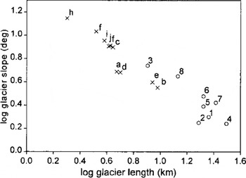
Fig. 4. Length and slope characteristics of eight normal glaciers predicted by the model to be of surge type with model fits higher than 0.7 (Nos. 1–8) and ten surge-type glaciers predicted by the model not to be of surge type with model fits smaller than 0.1 (letters a–j). A clear trend can be seen of increasing fit with glacier length as well as with decreasing glacier slope. For the glaciers with an intermediate length range of 8–13 km (log length 0.9–1.1), those with steeper slopes (Nos. 3 and 8) are predicted to be of surge type, and those with low slopes (e and b) to be non-surge-type. The numbers of normal glaciers are: 1. Zawadskibreen, 2. Mordsysselbreen, 3. Helsingborgbreen, 4. Sveabreen, 5. Petermannbreen, 6. Kantbreen, 7. Mordenskioldbreen, 8. Scheelebreen. Air-photo interpretation led to the reclassification of some of these as surge-type (Tables 5 and 6). The letters of surge-type glaciers are: a. Wandbreen, b. Werenskioldbreen, c. Scottbreen, d. Martinbreen, e. Pedasjenkobreen, f. Sør Crammerbreen, g. Livbreen, h. Arebreen, i. Plogbreen, j. Fyrisbreen.

Fig. 5. Surge evidence for Scheelebreen. (a) Part of 1956 air photo (S56 6060, © Norsk Polarinstitutt) showing the confluent tidewater margins of Scheele-, Paula- and Bakaninbreen at the head of van Mijenfjorden, southwest Spitsbergen. The lower 5 km of Scheelebreen is visible including an elongated moraine loop (see arrow). This loop originates at a western tributary (Luntebreen) 6 km from the margin (just off this photo, but visible on (b)). (b) Part of 1990 air photo (S90 3270, © Norsk Polarinstitutt) showing the lower 7 km of Scheelebreen. Since 1956, Scheelebreen has retreated 1.5 km and has become land-based. The elongated moraine loop has disappeared, but the tributary Luntebreen is forming a new loop while protruding onto the glacier surface (see arrow). At a next surge this loop will be elongated along with the trunk of Scheelebreen. Both air photos are at approximately the same scale. Although steady flow of Scheelebreen and periodic surging of Luntebreen could produce moraine loops, the typical tear shape of the moraine loop on the 1956 photo requires a surge of Scheelebreen for its formation.
Class B contains 55 glaciers (42% of the surge-type glaciers) with fitted values of 0.0–0.4. The length and slope characteristics of the ten surge-type glaciers with fits lower than 0.1 are shown in Figure 4 as comparison to the glaciers of class A with high model fits and surge characteristics. It is plausible that glaciers have stopped surging as a result of present mass-balance conditions (Reference Dowdeswell, Hodgkins, Nuttall, Hagen and HamiltonDowdeswell and others, 1995). Also, some of these might not be of surge type after all, but the observed advance might have been the Little Ice Age maximum, which occurred around 1900 in Svalbard (Reference Lefauconnier and HagenLefauconnier and Hagen, 1991). In total, 12 glaciers in class B had surges inferred in the period 1850–1936. We double checked the surge evidence of these glaciers in literature and on air photos, and concluded that Austre Brøggerbreen and Midre Lovénbreen did not have strong enough evidence to classify them as surge-type and hence reclassified these two as normal glaciers (see Table 6).
Table 6. Reclassification of the surge index based on logit model results and verification by air-photo interpretation

Glaciers in class B are located in three clusters, the first of which is in northwest Spitsbergen. All these surge-type glaciers are relatively small. A second cluster can be found in east Spitsbergen and Nordaustlandet: most surge-type glaciers in these areas are very large but have extremely low slopes. These findings agree with the observation that the ice-surface profiles of most Nordaustlandet surge-type glaciers lie below their theoretical profiles (Reference DowdeswellDowdeswell, 1986). As data collection at the compilation of the glacier inventory (1980–81; Reference Hagen, Liestøl, Roland and JørgensenHagen and others, 1993) might have been within a few decades after a surge or just prior to a surge, the overall slope and geometry of a glacier could be unfavourable for surging. For example, Palander- and Bodleybreen surged in 1969 and between 1970 and 1980, respectively (Reference Lefauconnier and HagenLefauconnier and Hagen, 1991). These glaciers might be building up to a new surge in the future, providing restriction of outflow and consequent steepening of the surface profile. Thirdly, most of the poorly fitting surge-type glaciers in southwest and north Spitsbergen overlie bedrock that is unfavourable to surging, such as the Precambrian metamorphic Hecla Hoek lithologies (Reference Hjelle and LauritzenHjelle and Lauritzen, 1982). However, plotting residuals against variables in the model did not reveal obvious over- or underprediction of specific variables, nor could we reveal additional controlling factors by the spatial analysis of residuals.
Reclassification of Glaciers and Model Results with the New Surge Classification
Results from the air-photo interpretation and model results of the optimal logit model led us to reclassify 25 glaciers in our database. Nineteen glaciers were added to the class of surge-type glaciers. Six glaciers were removed from that class because surge behaviour was not strong enough to state that a surge had happened in the past or is expected in the future (see Table 6). From the 504 glaciers a total of 145 are now classified as surge-type (S = 1) and 359 as normal (S = 0). This means that 14% of the glaciers larger than 1 km2 are of surge type. The location of the surge-type glaciers in Svalbard is given in Figure 6.

Fig. 6. Map of the Svalbard archipelago, with the updated distribution of surge-type glaciers in dark shading. The 145 surge-type glaciers include glaciers with an observed surge and those with clear morphological evidence of surge activity from air photos, satellite images, historical maps and publications. This distribution of surge-type glaciers represents the reclassified glacier data (S new ) in this paper. (This map is an update of Reference Dowdeswell, Hamilton and HagenDowdeswell and others, 1991, fig 1.)
A new logit model was fitted with the corrected classification (S new), as the changed values for the response variable might give different results in terms of environmental controls. Large changes were neither expected nor observed, as <5% of the glacier data were reclassified. The optimal model for S new (Table 7a) shows that the overall pattern of this new model is similar to the optimal model for S (Table 2): the parameter estimates changed only slightly. The only notable change is that now not only shale and mudstone but also other (coarser-grained) sedimentary bedrock is conducive to surging, although to a lesser extent than the fine-grained lithologies.
Table 7. (a) Optimal multivariate model for the distribution of surge-type glaciers based on the reclassified surge index (S new ). The reduction in model deviance is 218 for a loss of 10 degrees of freedom (χ2 crit = 18.3). A variable is significant at the 95% level (bold numbers) if the estimate is approximately twice the standard error (s.e.). (b) Optimal multivariate model for the distribution of surge-type glaciers based on only glaciers with measured RES and the corrected surge classification (S new ). The reduction in model deviance is 83 for a loss of 8 degrees of freedom (χ2 crit = 15.5)

We also fitted a new model with the S new classification for the RES-surveyed glaciers (Fig. 1). In this subset of 137 glaciers, 15 (11%) changed class. The main difference between the new IRH model (Table 7b) and the initial IRH model (Table 4b) is that AAR and elevation span are now included. However, the model reduction and parameter estimates for these variables are only just significant, so we should be careful with the physical interpretation of these mass-balance-related variables.
Discussion
Controls on glacier surging should reflect a number of conditions: (1) a net accumulation in the reservoir zone which is necessary for a glacier to build up to a new surge; (2) a restricted outflow causing the velocity to be lower than the balance velocity (Reference ClarkeClarke, 1987); and (3) the crossing of (a) glacier system threshold(s) at which ice flow becomes unstable. Measurements during the 1982–83 surge of Variegated Glacier, Alaska (Reference KambKamb and others, 1985), suggest that characteristics of the subglacial drainage system play an important role in surge development. Our model results indicate that for the 504 glaciers studied in Svalbard, long glaciers with relatively steep slopes overlying young sedimentary lithologies and orientations in a broad arc clockwise from northwest to southeast are most likely to be of surge type. We found that the significance of glacier length in the distribution of surge-type glaciers is not a proxy for the presence of geological boundaries as was suggested by Reference PostPost (1969) and Reference ClarkeClarke (1991).
The relationship between surging and glacier length and fine-grained sedimentary substrate could be explained in a number of ways. Firstly, there might be a causal relationship between subglacially derived debris content and surging (e.g. Reference ClappertonClapperton, 1975). Fine-grained sedimentary rocks are easily erodible, and till minerals derived from sedimentary rocks have a finer terminal grain-size than till minerals derived from, for example, metamorphic rocks (Reference Dreimanis, Vagners, Yatsu and FalconerDreimanis and Vagners, 1972; Reference BoultonBoulton, 1996). With increasing glacier length and thus a longer transport distance for particles, the till matrix becomes increasingly fine (Reference Dreimanis, Vagners, Yatsu and FalconerDreimanis and Vagners, 1972). The permeability of fine-grained tills is low and the deformation rate is very sensitive to small changes in pore-water pressure, grain-size distribution and mineralogy (Reference BoultonBoulton, 1979). As the thickness and permeability of a till layer is directly related to flow instability, the dynamic equilibrium of glaciers overlying fine-grained sedimentary beds could lead to surging behaviour (Reference Boulton and DobbieBoulton and Dobbie, 1993). Larger glaciers overlying fine-grained tills may therefore be most liable to surging behaviour (Reference BoultonBoulton, 1996).
Secondly, the increased surge probability of long glaciers could be explained by the distance-related attenuation of longitudinal stress (Kamb and Echelmeyer, 1987). Spatial variations in glacier movement are smoothed by longitudinal stress-gradient coupling related to glacier thickness in the form of a “longitudinal coupling length”, which is 1–3 times the glacier thickness for temperate valley glaciers (Reference Kamb and EchelmeyerKamb and Echelmeyer, 1986). Sinusoidal perturbations larger than 20 times the longitudinal coupling length are least attenuated. Since glacier length increases non-linearly with increasing glacier thickness (for a parabolic glacier profile length increases with the square increase in thickness), longer glaciers are more sensitive to longitudinal variations in movement between the upper and lower part of the glacier. These variations can be due to push-and-pull effects related to different throughput times of water in the accumulation and ablation areas (Reference Fountain and WalderFountain and Walder, 1998) or to the differential movement of the upper (increasingly active) and lower regions (increasingly stagnant) in the quiescent phase (Reference Robin and WeertmanRobin and Weertman, 1973). The larger stress gradients in these glaciers could lead to a damming effect and the development of a trigger zone for surging (Reference Robin and WeertmanRobin and Weertman, 1973).
A third explanation of the length–surging relation might lie in the polythermal regime of glaciers, which could be related to glacier size (Reference Hamilton and DowdeswellHamilton and Dowdeswell, 1996). Our models show that a polythermal regime is positively related to the distribution of surge-type glaciers. Recent observations on the thermal structure and surge development of Bakaninbreen, Svalbard, suggest that the propagation of the surge front is thermally controlled (Reference MurrayMurray and others, 2000). The boundary between warm and cold ice relates to the glacier geometry, controlling shear stress and basal water pressure and thus the basal movement. These results show that for Svalbard a thermally controlled surge mechanism is plausible.
A potential problem with the interpretation of IRH models is the cause-and-effect dilemma of thermal regime and glacier surging (Reference Clarke, Collins and ThompsonClarke and others, 1984; Reference Hamilton and DowdeswellHamilton and Dowdeswell, 1996). From our modelling of the IRH we can conclude that the presence of a polythermal regime could be a controlling factor for surging. However, from the models with IRH as response variable it appears that surging might control the presence of an IRH (Table 4b), so we cannot draw conclusions about the causality of the relationship. In the models with IRH as response variable it also appears that the IRHs occur preferentially in the western part of the archipelago. This suggests that other spatially distributed variables, i.e. temperature or precipitation, could be controlling the distribution of polythermal glaciers, (Reference BamberBamber, 1987a). Reference MacheretMacheret (1981) observed that the distribution of IRHs could be controlled by the regular decrease in glacier thickness on Spitsbergen going north and westward. We could not test these hypotheses as we have neither data available on glacier thickness nor glacier-specific data on precipitation or temperature. Moreover, we could not reveal significant correlations between glacier volume (a proxy for glacier thickness) and IRH, as glacier volume in our data is not a measured unit but is empirically calculated. The empirical formulas used to calculate glacier volume (Reference Hagen, Liestøl, Roland and JørgensenHagen and others, 1993) differentiate neither between surge-type and normal glaciers nor between thermal regimes of glaciers.
There are a number of additional complications in the interpretation of the results of the subset models of 137 RES glaciers. First, IRHs may not show up in glaciers that have recently surged, as the signal may be obscured by surface crevasses (Reference Dowdeswell, Drewry, Liestøl and OrheimDowdeswell and others, 1984). Further, a decrease in sample size will always result in a cruder picture of the nature of a population and a weaker manifestation of genuine relationships, not least because glacier attributes for the subset are not a fair representation of the total glacier dataset. Hence, the RES subset intrinsically generates different model results from the full set of glaciers. Further, the surveyed RES glaciers might introduce a sampling bias into the models.
The significant and positive correlation between surging and a higher than average surface slope can be used to argue against Reference KambKamb’s (1987) linked-cavity theory of surge behaviour since this theory predicts that glaciers with low surface slopes are most likely to be of surge type (Reference ClarkeClarke, 1991). Our slope results lend no support to the linked-cavity mechanism of glacier surging being prevalent in Svalbard. The IRH, lithology and length results imply a thermally controlled soft-bed surge mechanism.
A number of questions remain. As all studies, including this one, reveal that long glaciers have high surge probabilities, why are not all glaciers exceeding a certain length in a cluster region of surge type? On the other hand, which specific conditions are required to make some very small glaciers surge? Study of the specific characteristics of small surge-type glaciers might elucidate controls of surging hitherto overlooked.
Summary and Conclusions
Our analysis attempted to explore and quantify the relations between surge-type glaciers and glacial and environmental variables by isolating factors that distinguish surge-type glaciers from normal glaciers. We identified a combination of independent factors that appear to be related to surging in multiple regression (logit) models. The data analysis and results presented in this paper show that:
For the full dataset of 504 glaciers: long glaciers with slopes above average, orientations in a broad arc from northwest to southeast and overlying young fine-grained sedimentary lithologies are most likely to be of surge type.
For the subset of 137 glaciers with measured RES: long glaciers with large elevation spans, AARs close to balance, polythermal regimes and overlying sedimentary lithologies are most likely to be of surge type.
These results support a thermally controlled soft-bed surge mechanism for Svalbard. We also explored the contributions of individual glaciers to the statistical model, and fitted surge probabilities for individual glaciers based on the glacial and environmental characteristics of these glaciers. As the prediction of surge-type glaciers by the logit model leads to a much higher percentage of detected surge features than a random air-photo interpretation, it seems that the criteria used in the model are indeed related to surging. Our optimal model could therefore be used to predict surge probabilities of glaciers not included in our analysis. Finally, detailed study of the group of irregular or “unusual” surge-type glaciers identified through our residual analysis could give further clues to controls on surging. These studies might also provide insight into the role of glacier length and substrate properties in glacier dynamics.
Acknowledgements
The Norsk Polarinstitutt, Oslo, is thanked for access to its air-photo and map archives. Discussions with J. O. Hagen on Svalbard surges were valuable and much appreciated. We thank P. Jansson and G. K. C. Clarke for their constructive criticism of a draft manuscript of this paper. All logit models were run on the MIDAS CS6400 at the Manchester Computer Centre. H.J. was funded through a School of Geography, University of Leeds scholarship.


