


1. Introduction
Turbulent line plumes emerge from long, slender sources. Their widespread occurrence in natural and built environments has motivated numerous previous studies, including those concerned with pollutant transport (Koh & Brooks Reference Koh and Brooks1975), eruptions from volcanic fissures such as Laki in 1783 in Iceland (Stothers Reference Stothers1989), convective flows from both glacial leads and burning buildings (Ching, Fernando & Noh Reference Ching, Fernando and Noh1993; Yokoi Reference Yokoi1960) and ocean stratification (Wells & Wettlaufer Reference Wells and Wettlaufer2005). Due to the turbulent entrainment of fluid from the surrounding environment, the physical scale of these buoyancy-driven flows increases with distance from the source. As such, the rate of entrainment into a line plume is instrumental to their fundamental behaviour and successful prediction.
Two-dimensional mathematical models for idealised turbulent line plumes from sources of infinite length have been developed (Batchelor Reference Batchelor1954; Lee & Emmons Reference Lee and Emmons1961; van den Bremer & Hunt Reference van den Bremer and Hunt2014a). A crucial component of these models is the turbulence closure that relates the velocity of entrained ambient fluid to a characteristic vertical velocity in the plume (Morton, Taylor & Turner Reference Morton, Taylor and Turner1956). While appearing in plume theory in multiple conventions (Lee & Emmons Reference Lee and Emmons1961; van den Bremer & Hunt Reference van den Bremer and Hunt2014a; Paillat & Kaminski Reference Paillat and Kaminski2014a), following Lee & Emmons (Reference Lee and Emmons1961) we express this closure using the entrainment coefficient  $\alpha$ such that the horizontal entrainment velocity $u_e$ is related to the time-averaged centreline velocity of the plume $w_c$ via
 \begin{equation} u_e = \alpha w_c. \end{equation}
Although line plumes have been studied since Rouse, Yih & Humphreys (Reference Rouse, Yih and Humphreys1952), a consensus has not been reached regarding the value of the entrainment coefficient  $\alpha$, even for the simplest case: a line plume in equilibrium in unstratified quiescent surroundings where dimensional arguments show that $\alpha$ should be a constant. Summary tables of experimental measurements produced by Yuan & Cox (Reference Yuan and Cox1996), van den Bremer & Hunt (Reference van den Bremer and Hunt2014a) and Parker et al. (Reference Parker, Burridge, Partridge and Linden2020) report $0.11\leq \alpha \leq 0.20, 0.10\leq \alpha \leq 0.16$ and
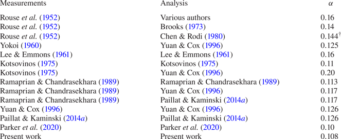
  $0.10\leq \alpha \leq 0.16$, respectively. Table 1 collates all the reported values that we could trace back to experimental measurements. This wide range, with a variation of $100\,\%$ between the minimum and maximum, does not engender confidence in predictions of plume behaviour. For example, based on classic plume theory, the distance at which fluid in the plume has diluted to a given value varies by up to $60\,\%$ depending on the choice of $\alpha$ from this table.
Table 1. Values of the entrainment coefficient, defined by (1.1), reported for a turbulent line plume. Entries have been converted from different plume theory conventions when necessary. First column: the author(s) who report the original data. Second column: the author(s) who report a value for  $\alpha$ based on an independent analysis of the original data. Rouse et al. (Reference Rouse, Yih and Humphreys1952) do not give a value for $\alpha$ as their work was published before Morton et al. (Reference Morton, Taylor and Turner1956) introduced the entrainment hypothesis (1.1), but their reported measurements imply $\alpha =0.16$. $^\circ$Chen & Rodi (Reference Chen and Rodi1980) do not report a value for $\alpha$, but this entry is consistent with their analysis, unlike values closer to $0.13$ occasionally attributed to them (Yuan & Cox Reference Yuan and Cox1996; van den Bremer & Hunt Reference van den Bremer and Hunt2014a). The data underpinning the values listed above are analysed in § 4, and a summary of revised values for $\alpha$ is given in table 4.
The uncertainty surrounding the value of  $\alpha$ can also be linked to two factors highlighted by table 1. First, there is a general scarcity of experimental data on line plumes – to date only eight independent datasets (nine, including our own (§ 5)) have been used to calculate $\alpha$. Second, for three of these datasets, a subsequent analysis by other authors has led to conflicting values of $\alpha$ being published for the same data – note the table entries for Rouse et al. (Reference Rouse, Yih and Humphreys1952), Kotsovinos (Reference Kotsovinos1975) and Ramaprian & Chandrasekhara (Reference Ramaprian and Chandrasekhara1989).
There are suggestions or recommendations for a particular value of  $\alpha$ within the range $0.1$– $0.2$. Yuan & Cox (Reference Yuan and Cox1996), although acknowledging the wide range in values, recommend $\alpha =0.13$. Based on the Poreh et al. (Reference Poreh, Morgan, Marshall and Harrison1998) data for two-dimensional spill plumes, created by a gravity current that ‘spills’ over the end of a horizontal boundary, Thomas, Morgan & Marshall (Reference Thomas, Morgan and Marshall1998) show that a line plume model with $\alpha =0.11$ describes the far-field plume. Given the non-zero horizontal momentum flux, one cannot automatically assume that an entrainment coefficient derived from spill plume data captures the behaviour of classic line plumes, although $\alpha =0.11$ sits firmly within the range reported (table 1) and Thomas et al. (Reference Thomas, Morgan and Marshall1998) recommended its use in fire safety models. Paillat & Kaminski (Reference Paillat and Kaminski2014a) only compare their measurements with Ramaprian & Chandrasekhara (Reference Ramaprian and Chandrasekhara1989), commenting on the good agreement, implicitly suggesting $\alpha =0.12$. Clearly, no consensus has been reached on the most appropriate value of $\alpha$, as highlighted by recent comments on the significant spread in reported values (Kaye & Cooper Reference Kaye and Cooper2018; Parker et al. Reference Parker, Burridge, Partridge and Linden2020).
The lack of consensus is not just problematic for the accuracy of predictions based on classic plume theory. A consensus value for  $\alpha$ would also greatly benefit the analysis of non-equilibrium forced and lazy plumes (Lee & Emmons Reference Lee and Emmons1961; van den Bremer & Hunt Reference van den Bremer and Hunt2014a). It is well accepted (Kotsovinos Reference Kotsovinos1975; Kotsovinos & List Reference Kotsovinos and List1977; Yannopoulos Reference Yannopoulos2006; van den Bremer & Hunt Reference van den Bremer and Hunt2014a; Paillat & Kaminski Reference Paillat and Kaminski2014a) that the entrainment coefficient of a line plume is about twice that of a line jet, despite reported values for a line plume showing the same factor of two difference. Similarly, an improved reference value for $\alpha$ could aid the development and enable experimental verification of more complex plume models such as those considering non-Boussinesq effects (van den Bremer & Hunt Reference van den Bremer and Hunt2014b) or self-similarity drift (Paillat & Kaminski Reference Paillat and Kaminski2014a). Wall plumes, resulting from either a vertically distributed source of buoyancy or a line source at the base of the wall, are commonly compared with line plumes (Grella & Faeth Reference Grella and Faeth1975; Baines Reference Baines2002; Kaye & Cooper Reference Kaye and Cooper2018; Parker et al. Reference Parker, Burridge, Partridge and Linden2020). However, efforts to establish the quantitative effect of the wall on entrainment are clearly hindered by the uncertainty in $\alpha$. Understanding and predicting the transition of a free plume from near-field line-like behaviour to an axisymmetric asymptotic state would also benefit from a well-established value for $\alpha$ (Yokoi Reference Yokoi1960). In order to better understand these related flows and improve the predictions of line plume models we require an answer to the broader question: what is the entrainment coefficient of a pure turbulent line plume?
We address this question with a multi-faceted approach. First, we review and extend the plume model developed by Lee & Emmons (Reference Lee and Emmons1961) and Yuan & Cox (Reference Yuan and Cox1996), placing an emphasis on the relationships between plume measurements and calculated values of the entrainment coefficient. These relationships reveal non-trivial links between uncertainties in measured quantities and uncertainties in the calculated values of  $\alpha$ which illuminate both experimental design and the analysis of past experiments. Second, using this theoretical framework, we assess the literature to identify the reasons for the variation in past measurements of $\alpha$. Our analysis leads us to conclude that the value for $\alpha$ falls within a considerably smaller range than suggested by table 1. Third, using our theoretical framework as a guide, we design an experiment which enables $\alpha$ to be determined more precisely than in past studies. Our measurements of the entrainment velocity into a turbulent saline plume are a first in this context and, combined with measurements of the scalar field, lead us to deduce $\alpha =0.108$. This value is in good agreement with the new understanding of the literature and we conclude that, based on all the evidence, $\alpha =0.11\pm 15\,\%$.
2. Theoretical framework
2.1. Plume theory
Consider a turbulent plume that develops from an infinitely long slender source of buoyancy flux per unit length  $B_0$ (dimension L $^3$T
$^3$T $^{-3}$, where L is length and T is time), in an otherwise quiescent and miscible environment of uniform density $\rho _e$, subject to the gravitational acceleration $g$. Let the vertical coordinate $z$ denote the distance from the source in the streamwise direction, $x$ the cross-stream coordinate where $x=0$ is the plume centreline and $y$ the spanwise coordinate. The effect of the buoyancy force, characterised by the buoyancy of the plume relative to the environment $g'=g(\rho _e-\rho )/\rho _e$, where $\rho$ is the local density of the plume, is to induce a vertical velocity $w$. Here, $g'$ and $w$ are the time- and spanwise-averaged quantities at a point ( $x,z)$.
As is standard, the integral fluxes of volume  $Q$ (L $^2$T
$^2$T $^{-1}$), specific momentum $M$ (L $^3$T
$^3$T $^{-2}$) and buoyancy $B$ through a horizontal cross-section are then defined as
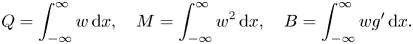 \begin{equation} Q=\int_{-\infty}^{\infty} w\,\mathrm{d} x , \quad M=\int_{-\infty}^{\infty} w^2\,\mathrm{d} x, \quad B=\int_{-\infty}^{\infty} wg'\, \mathrm{d} x.\end{equation}
Following the assumptions made to the Navier–Stokes equations by Morton et al. (Reference Morton, Taylor and Turner1956) and Lee & Emmons (Reference Lee and Emmons1961), the plume is modelled by conservation equations for these integral quantities. For an unstratified environment these are
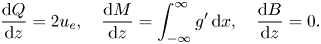 \begin{equation} \frac{\mathrm{d} Q}{\mathrm{d} z} =2u_e, \quad \frac{\mathrm{d} M}{\mathrm{d} z} =\int_{-\infty}^{\infty}g'\, \mathrm{d} x, \quad \frac{\mathrm{d} B}{\mathrm{d} z} =0.\end{equation}
To close (2.2a–c), we must specify the cross-plume variation of  $w$ and $g'$ and relate $u_e$ to the integral quantities. It is at this stage that various conventions for the entrainment coefficient are introduced. One convention assumes ‘top-hat’ profiles whereby the plume is modelled as having a uniform average velocity $w_T=M/Q$ and buoyancy $g_T'=B_0/Q$ across a finite width $2b_T=Q^2/M$ and zero vertical velocity and buoyancy outside. The top-hat entrainment coefficient $\alpha _T$ is then defined such that $u_e=\alpha _T M/Q$. A second convention, based on observations that the time-averaged cross-stream profiles of velocity and buoyancy are self-similar and Gaussian-like (Rouse et al. Reference Rouse, Yih and Humphreys1952; Kotsovinos Reference Kotsovinos1975; Ramaprian & Chandrasekhara Reference Ramaprian and Chandrasekhara1989; Paillat & Kaminski Reference Paillat and Kaminski2014a; Parker et al. Reference Parker, Burridge, Partridge and Linden2020), assumes that the profiles are the Gaussians
 \begin{equation} w(x,z)=w_c(z)\exp{\left(-\frac{x^2}{b^2}\right)}, \quad g'(x,z)=g'_c(z)\exp{\left(-\frac{x^2}{(\lambda b)^2}\right)}. \end{equation}
In (2.3a,b),  $g'_c$ is the centreline buoyancy and $b$ and $\lambda b$ are the characteristic half-widths of the profiles where the velocity and buoyancy, respectively, drop to $1/e$ (where $\ln {e}=1$) of the centreline value. Experimental measurements show that the buoyancy profile is wider than the velocity profile, i.e. the profile coefficient $\lambda >1$ (e.g. Ramaprian & Chandrasekhara Reference Ramaprian and Chandrasekhara1989). Via (2.1a–c), these profiles correspond to the integral quantities
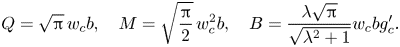 \begin{equation} Q=\sqrt{\rm \pi}\,w_cb, \quad M=\sqrt{\frac{\rm \pi}{2}}\,w_c^2b, \quad B=\frac{\lambda\sqrt{\rm \pi}}{\sqrt{\lambda^2+1}} w_c b g'_c. \end{equation}
For the idealised case of a true line plume source, the source volume and momentum fluxes are zero and the plume is in an asymptotic state whereby  $\alpha$ (or $\alpha _T)$ and $\lambda$ are constants for any $z>0$. Solution of (2.2a–c) for this idealised case, based on the top-hat convention, yields
 \begin{equation} Q=(2\alpha_T)^{2/3}B_0^{1/3}z , \quad M=(2\alpha_T)^{1/3}B_0^{2/3}z, \quad B=B_0,\end{equation}
and based on the Gaussian convention
 \begin{equation} Q=2^{5/6}(1+\lambda^2)^{1/6}\alpha^{2/3}B_0^{1/3}z, \quad M=2^{1/6}(1+\lambda^2)^{1/3}\alpha^{1/3}B_0^{2/3}z, \quad B=B_0.\end{equation}
Clearly, there is a requirement that  $Q, M$ and $u_e$ be identical irrespective of the form of the profile assumed and, thus, the values of $\alpha _T$ and $\alpha$ are linked. For example, $\alpha _T=\sqrt {2}\alpha$ on taking ${\lambda =1}$ as is a typical simplification in the top-hat model (van den Bremer & Hunt Reference van den Bremer and Hunt2014a; Paillat & Kaminski Reference Paillat and Kaminski2014a). This link is outlined here given top-hat profiles are widely adopted in applications of classic plume theory. However, for interpreting experimental measurements, it is convenient to work using the Gaussian convention as the majority of the reported values for $\alpha$ (table 1) were calculated from fits to measured Gaussian-like time-averaged velocity and buoyancy profiles.
On dimensional grounds, the characteristic velocity profile half-width, centreline velocity and centreline buoyancy of a turbulent plume from a line source can be expressed as
 \begin{equation} b=C_bz, \quad w_c=C_w B_0^{1/3}, \quad g_c'=C_g B_0^{2/3} z^{{-}1}, \end{equation}
where  $C_b, C_w$ and $C_g$ are dimensionless coefficients. Equating (2.4a–c) with (2.6a–c) and substituting for (2.7a–c) shows that these coefficients are related to $\alpha$ and $\lambda$ as follows:
 $$\begin{gather} \sqrt{\rm \pi} C_wC_b =2^{5/6}(1+\lambda^2)^{1/6}\alpha^{2/3}, \end{gather}$$
 $$\begin{gather}\sqrt{\rm \pi} C_w^2C_b =2^{2/3}(1+\lambda^2)^{1/3}\alpha^{1/3}, \end{gather}$$
 $$\begin{gather}\sqrt{\rm \pi} C_w C_g C_b =\lambda^{{-}1} (1+\lambda^2)^{1/2} . \end{gather}$$
These three coupled algebraic equations, expressed in similar forms by Lee & Emmons (Reference Lee and Emmons1961) and Yuan & Cox (Reference Yuan and Cox1996), have five unknowns. Thus, the measurement of a pair of coefficients is necessary before  $\lambda$, the remaining coefficients and our ultimate target, $\alpha$, can be deduced. The pairings are not limited to the coefficients appearing in (2.8)–(2.10), and at this stage it is convenient to define the following four coefficients:
 \begin{equation} \lambda b=C_{\lambda b}z, \quad Q=C_Q B_0^{1/3}z, \quad M=C_M B_0^{2/3}z, \quad u_e=C_e B_0^{1/3}. \end{equation}
These coefficients are readily linked to  $\alpha$ and $\lambda$ following substitution into (2.8)–(2.10) via (1.1), (2.6a–c) and (2.7a–c).
2.2. Determining  $\alpha$ and $\lambda$


Only a small fraction of all the possible pairings of coefficients have been used previously to determine  $\alpha$ and $\lambda$. Kotsovinos (Reference Kotsovinos1975) and Paillat & Kaminski (Reference Paillat and Kaminski2014a) used the pair $(C_{b},C_{\lambda b})$, i.e. measurements of the widths of the velocity and buoyancy profiles. Rearrangement of (2.8) and (2.9), and the definition of $\lambda$, leads to
 \begin{equation} \alpha=\frac{\sqrt{\rm \pi}}{2}C_b, \quad \lambda =\frac{C_{\lambda b}}{C_b}. \end{equation}
The straightforward forms of (2.12a,b) plausibly explains why the pair  $(C_{b},C_{\lambda b})$ is one of the most commonly selected to determine $\alpha$ and $\lambda$. Notably, only measurement of $C_b$ is needed to estimate $\alpha$.
In contrast, Yuan & Cox (Reference Yuan and Cox1996) designed their experiment to determine  $\alpha$ and $\lambda$ (Yuan & Cox (Reference Yuan and Cox1996) use $\beta =1/\lambda ^2$) from measurements of the centreline velocity and buoyancy, i.e. the pair $(C_w,C_g)$. For this pairing, (2.8) and (2.10) lead to the more complex relationships
 \begin{equation} \alpha=\frac{\sqrt{2C_g^2+C_w^4}}{2C_w^3C_g}, \quad \lambda =\frac{C_w^2}{\sqrt{2}C_g}. \end{equation}
Yuan & Cox (Reference Yuan and Cox1996) used this pair to calculate a value of  $\alpha$ (and $\lambda$) from measurements made by themselves and others – note the entries in table 1 linked to their analysis. In doing so, they appear to have been the first authors to reexamine past data by using a different coefficient pair than the original experimentalist(s).
There are  $\binom{5}{2}=10$ possible pairings of the five most commonly measured coefficients $C_b, C_{\lambda b}, C_w, C_g$ and $C_Q$; the expressions for these pairings are listed in Appendix A. In addition to $(C_{b},C_{\lambda b})$ and ${(C_{w},C_{g})}$, only two more of the possible pairings have been chosen previously to determine $\alpha$ and $\lambda$, namely, ${(C_{\lambda b},C_{g})}$ by Lee & Emmons (Reference Lee and Emmons1961) and ${(C_{w},C_{Q})}$ by Ramaprian & Chandrasekhara (Reference Ramaprian and Chandrasekhara1989). Our measurements of $C_e$ (§ 5) can be related to $\alpha$ and $\lambda$ via relationships involving $C_Q$: the change in volume flux being the result of entrainment into the two sides of the plume ( $C_Q=2C_e$). We additionally include the relationships for two pairs involving the coefficients $C_M$ and $C_B=w_cg'_cz/B_0$, although do not include every possible combination. The pair ${(C_{M},C_{Q})}$ is closely linked to the top-hat plume width measured by Parker et al. (Reference Parker, Burridge, Partridge and Linden2020). The pair ${(C_{g},C_{B})}$ uses centreline measurements of the buoyancy and the product of the buoyancy and velocity, and highlights how experimental capabilities could motivate the study of additional pairs; in this case, possibly using a combined temperature and heat-flux sensor.
3. Quantifying the consequences of experimental error
Given there are numerous ways that an experiment could be designed, a key question arises: of the possible coefficient pairs, is there a specific pair that should be targeted in order to best determine  $\alpha$? In particular, are there pairings that are less susceptible to experimental uncertainty and, thereby, will yield more reliable estimates for $\alpha$?
Assuming that random measurement errors are small and uncorrelated, the uncertainty in the value of  $\alpha$ calculated from the pair $(C_1,C_2)$ is
 \begin{equation} \delta \alpha=\sqrt{\left(\frac{\partial \alpha}{\partial C_1}\delta C_1\right)^2+\left(\frac{\partial \alpha}{\partial C_2}\delta C_2\right)^2}, \end{equation}
where  $\delta$ indicates an uncertainty in the quantity, such as the standard deviation or the width of a confidence interval. This assumption may not be strictly true depending on the experimental approach deployed. For example, $C_w$ and $C_Q$ will be correlated if both are determined from measurements of the velocity profile, but could be uncorrelated if $C_Q$ were instead determined using a technique to measure the volume flux directly (Zukoski, Kubota & Cetegen Reference Zukoski, Kubota and Cetegen1981; Baines Reference Baines1983).
We are relatively unconcerned whether it is more appropriate to sum uncertainties linearly or in quadrature, and are not suggesting that all past measurements should be rigorously analysed within this framework. Indeed, most studies consist of a relatively small number of individual experiments or do not report standard deviations, hindering detailed interpretation, statistical or otherwise. Nevertheless, the partial derivatives account for the sensitivity of  $\alpha$ to changes in the coefficient values, even if it is unclear whether the uncertainties should be added in quadrature.
A similar expression to (3.1) can be written for  $\delta \lambda$. For every coefficient pair, the required partial derivatives can be evaluated and expressed in the normalised forms
 \begin{equation} \frac{\delta\alpha}{\alpha}=\sqrt{k_1^2 \left(\frac{\delta C_1}{C_1}\right)^2+k_2^2 \left(\frac{\delta C_2}{C_2}\right)^2}, \quad \frac{\delta\lambda}{\lambda}=\sqrt{k_3^2 \left(\frac{\delta C_1}{C_1}\right)^2+k_4^2 \left(\frac{\delta C_2}{C_2}\right)^2}, \end{equation}
where we refer to the positive values of  $k_i, i=\{1,\ldots,4\}$, as uncertainty multipliers. The expressions for $k_i$ for each coefficient pair are listed in Appendix A. While $k_i$ can be evaluated using measurements from a particular experiment, for the purpose of calculating the representative uncertainty multipliers presented in table 2, we use the coefficient values that can be calculated from $\alpha =0.11$ and $\lambda =1.2$, the values that we conclude (§ 7) best represent the available experimental evidence. These values for $\alpha$ and $\lambda$ yield the following set: $C_b=0.1241, C_{\lambda b}=0.1489, C_w=2.157, C_g=2.743$ and $C_Q=0.4746$ (to four significant figures (s.f.) to minimise rounding errors).
Table 2. (a) Estimates of the uncertainty multiplier  $k_1$ for a given pair $(C_1,C_2)$ used to calculate $\alpha$. (b) Estimates of the uncertainty multiplier $k_3$ for a given pair $(C_1,C_2)$ used to calculate $\lambda$. Values are either integers or reported to two decimal places. As $C_Q=2C_e$, conclusions drawn regarding the uncertainty multipliers for $C_e$ are identical to those for $C_Q$.
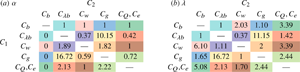
The entries in table 2 are the uncertainty multipliers for  $C_1$ when paired with $C_2$. For example, to calculate the uncertainty in $\alpha$ determined from the pair ${(C_{\lambda b},C_{w})}$, the uncertainty in the measurements of $C_{\lambda b}$ is multiplied by $k_1=0.37$ (reading off table 2(a) using $C_1=C_{\lambda b}$ and $C_2=C_{w}$ (purple entries)). Reversing the order and setting $C_1=C_w$ and $C_2=C_{\lambda b}$, the multiplier for $C_w$ when paired with $C_{\lambda b}$ is $k_1=1.89$.
The links between a pair of coefficients and  $\alpha$ and $\lambda$ are, in general, nonlinear, and the use of the truncated Taylor series to express (3.2a,b) will introduce some error. The significance of this error will depend on the given measurements for a pair, but a more considered calculation of the uncertainty – for example, using higher-order terms in the Taylor series approximation – may be necessary in certain cases. Nevertheless, the uncertainty multipliers in table 2 provide immediate insight into the implications of selecting a given coefficient pair and, thereby, a particular experimental approach. First, consider the example pairing ${(C_{e},C_{\lambda b})}$, i.e. the red entries in table 2(a). In this case, the estimate for $\alpha$ is clearly dominated by the uncertainty in $C_e$, as the square of its multiplier exceeds that for $C_{\lambda b}$ by a factor of $(2.13/0.42)^2\approx 26$. In a similar vein, the direct link between $C_b$ alone and $\alpha$ (2.12a) is indicated in table 2(a) by $k_1=0$ for any other coefficient paired with $C_b$. Second, while the majority are broadly comparable in magnitude, the uncertainty multipliers for ${(C_{\lambda b},C_{g})}$ stand out as being considerably larger. Thus, the pairing ${(C_{\lambda b},C_{g})}$ would not be a wise choice to determine $\alpha$, unless particularly precise measurements of the buoyancy field could be made. Indeed, in light of this uncertainty analysis it is ironic that, of the six datasets which only include two coefficients, four measure the pair ${(C_{\lambda b},C_{g})}$ (Lee & Emmons Reference Lee and Emmons1961; Harris Reference Harris1967; Anwar Reference Anwar1969; Sangras, Dai & Faeth Reference Sangras, Dai and Faeth1998), although we note these experimentalists were not focused on determining $\alpha$. With reference to table 2(b), similar deductions can be made concerning the multipliers that underlie the uncertainty in $\lambda$.
We do not assert that the uncertainty multipliers in table 2 dictate that a particular coefficient pair should be chosen. Many of the multipliers are similar in value, and differences in how precisely a coefficient can be determined will also have an impact. It is also unlikely that experimentalists would agree on whether it is preferable to measure two coefficients relatively well, or choose a pair where one coefficient can be the focus of the measurement campaign. However, if one could make good estimates for how precisely each coefficient could be measured, then the uncertainty multipliers would point to a particular pair. At the very least, the multipliers should play a guiding role in experimental design.
In what follows, further insights gained from the uncertainty multipliers are brought to bear, both in our assessment of past experiments (§ 4) and in informing the design of our original new experiments (§ 5) that centre around the evaluation of a previously unconsidered coefficient pair.
4. Experimental data assessment
Given  $\alpha$ is not measured directly, further investigation into the variation of the values reported for $\alpha$ requires consideration of the variation in the underlying measurements. These are recorded in table 3 with the pertinent experimental details, including the source length $L$ and width $s=2b_0$ (where $b_0$ is the physical half-width of the source), the vertical position of the measurement region $z_m$ and the presence, or otherwise, of end walls.
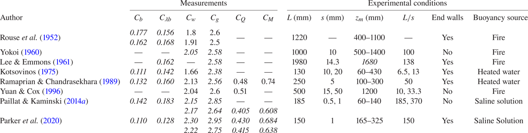
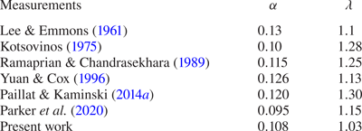
Table 3. Summary of experimental measurements used to calculate  $\alpha$ and the corresponding experimental conditions. Single-valued entries for $z_m$ imply the measurement region extended from near the source to the upper bound given; the reported coefficient values were determined only from the region where far-field plume behaviour was demonstrated. Entries in italics (given to 3 s.f.) indicate that we performed some manipulation or calculation on the information from the original literature source. A majority of the calculations were simply algebraic to switch to the convention used herein or to work backwards from given values of $\alpha$ and $\lambda$. Entries for $C_w$ and $C_g$ from Paillat & Kaminski (Reference Paillat and Kaminski2014a) and $z_m$ from Lee & Emmons (Reference Lee and Emmons1961) involved estimating values from their plots. The Kotsovinos (Reference Kotsovinos1975) entries for $C_b$ and $C_{\lambda b}$ were calculated from their plume width data (Appendix C). The entries for Parker et al. (Reference Parker, Burridge, Partridge and Linden2020) were calculated from provided data (§ 4.7 and Appendix D); the multiple entries for four of the coefficients are because three different representative buoyancy fluxes (source, mean and total) were used to normalise the measurements. The second row of entries for Rouse et al. (Reference Rouse, Yih and Humphreys1952) are revised fits to their measurements proposed by Chen & Rodi (Reference Chen and Rodi1980) (see § 4.2). Rouse et al. (Reference Rouse, Yih and Humphreys1952) state that the heat source is line like, but do not report on the source width.
A cursory examination of table 3 reveals that the range of reported values for  $\alpha$ is not simply a result of different interpretations of the measurements: the measurements alone show considerable variation. For example, measurements of $C_b$ vary by $60\,\%$ across the experiments which is noteworthy as many reported values for $\alpha$ are calculated using $C_b$. Given the broad range of experimental conditions used to study line plumes (table 3), our assessment of the experimental data continues by considering whether there is any systematic link between the experimental geometry and the reported values of $\alpha$.
4.1. Effects of experimental conditions
It is natural to enquire if the reported variations in  $\alpha$ can be attributed to differences in how ‘line like’ the experimental set-ups were. In an ideal scenario, measurements would be made from a long and slender source ( $L/s\gg 1$) at downstream distances $z_m$ that are small relative to the source length ( $L/z_m \gg 1$) and large relative to the source width ( $z_m/s \gg 1$). Practically, it is infeasible to insist that $s \ll z_m \ll L$ and, consequently, experimentalists are forced to compromise on what conditions are appropriate. In general, an experiment can be deemed increasingly ‘line like’ if the ratios $L/s, L/z_m$ and $z_m/s$ are larger, and if there are end walls to encourage a two-dimensional induced-flow field.
The variation in the reported values for  $\alpha$ with the experimental geometry is shown in figure 1. There is no clear evidence in these plots for a systematic relationship between how line-like experiments are and the value of $\alpha$. Further support for this claim is provided by Yuan & Cox (Reference Yuan and Cox1996) and Paillat & Kaminski (Reference Paillat and Kaminski2014a) whose measurements of plumes from sources of two different widths show no systematic difference in the centreline properties.
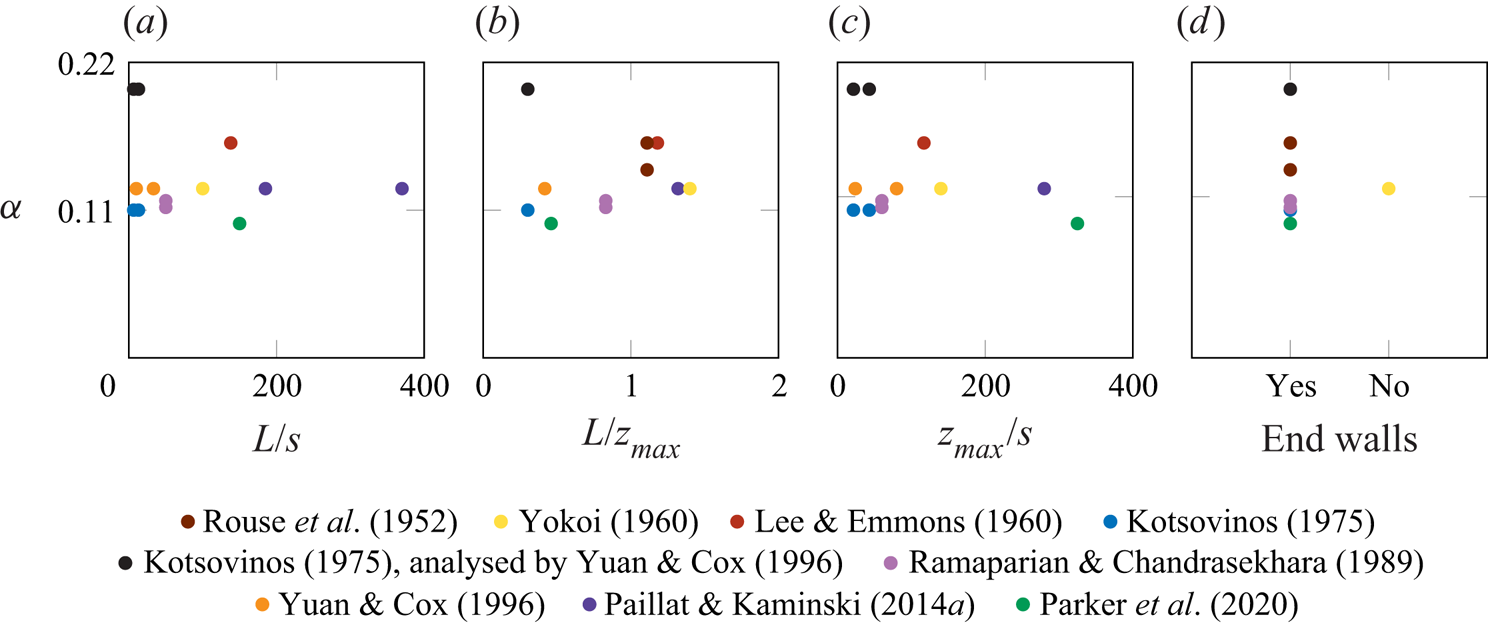
Figure 1. Variation of the reported values for  $\alpha$ with experimental geometry. (a) $\alpha$ vs the source aspect ratio $L/s$; both values for $L/s$ are shown where two aspect ratios were studied, (b) $\alpha$ vs the source length $L$ scaled on the largest downstream distance that measurements are reported $z_{max}$, (c) $\alpha$ vs $z_{max}$ scaled on the source width; both values are shown where two different source widths were used, (d) The presence of end walls; note that three ‘No’ data points overlap (Yokoi Reference Yokoi1960; Yuan & Cox Reference Yuan and Cox1996; Paillat & Kaminski Reference Paillat and Kaminski2014a).
In addition to plumes from a large aspect ratio line-like source, Yokoi (Reference Yokoi1960) studied plumes from sources with  $L/s=1.4, 2.7$ and $5.5$. His measurements of $g'_c$ above these small aspect ratio sources show that the departure from the two-dimensional scaling ( $g'_c \sim z^{-1}$) toward the axisymmetric scaling ( $g'_c \sim z^{-5/3}$) occurs for $z/L\approx 6 - 7$. As all of the experiments reported in table 3 have sources with $L/s > 5.5$ and only report measurements for $z/L \lesssim 3$, the apparent absence of systematic effects due to the source geometry is not surprising.
While in principle there should be no difference between measurements of dynamically equivalent plumes in water or air, possible systematic differences can be identified. For example, plumes above a fire source are subject to non-Boussinesq effects (van den Bremer & Hunt Reference van den Bremer and Hunt2014b) while those in water tanks will be affected by the confining walls and filling-box effects (Baines & Turner Reference Baines and Turner1969; Barnett Reference Barnett1991). A brief analysis suggests that the fire plume measurements reported in table 3 were unaffected by non-Boussinesq effects (Appendix B). In contrast, confinement effects could not be ruled out, and we discuss their possible impact on  $\alpha$ in § 6; however, we did not identify a systematic variation due to confinement. Other possible effects, such as similarities in the design of the source, or measurement instrumentation and techniques, were not considered (and because of the small number of measurements, it is not clear that such an analysis would be fruitful).
As the variation in  $\alpha$ cannot be explained by systematic differences between the experiments, we proceed by analysing the experimental campaigns in turn (§§ 4.2–4.7). We summarise the main findings in § 4.8 where we present a new curated table of values for $\alpha$ (table 4). Although some of the changes are relatively minor, the analysis results in several significant modifications. In particular, we identify an alternative (and more appropriate) value for $\alpha$ using the measurements of Lee & Emmons (Reference Lee and Emmons1961) and we reject the value that Yuan & Cox (Reference Yuan and Cox1996) attribute to Kotsovinos (Reference Kotsovinos1975). As a result, we show that $0.095\lesssim \alpha \lesssim 0.13$ is a better representation of the variation in past measurements.
Table 4. Updated list of values for the entrainment coefficient and profile coefficient of a turbulent line plume following analysis of the literature. Summary of differences from table 1: erroneous values for Lee & Emmons (Reference Lee and Emmons1961) and Kotsovinos (Reference Kotsovinos1975) have been removed; entries for Rouse et al. (Reference Rouse, Yih and Humphreys1952) and Yokoi (Reference Yokoi1960) have been removed because of concerns regarding the interpretation of their data; based on consideration of multiple coefficient pairs, the entries for Ramaprian & Chandrasekhara (Reference Ramaprian and Chandrasekhara1989), Paillat & Kaminski (Reference Paillat and Kaminski2014a) and Parker et al. (Reference Parker, Burridge, Partridge and Linden2020) are now a single representative value.
4.2. Rouse et al. (Reference Rouse, Yih and Humphreys1952)
Rouse et al. (Reference Rouse, Yih and Humphreys1952) measured  $w(x)$ and $g'(x)$ at different heights in a thermal plume created by a line of gas burners. Although they do not calculate $\alpha$, the coefficients $C_b, C_{\lambda b}, C_w$ and $C_g$ can be determined from their reported profiles. These profiles were chosen to fit their measurements subject to constraints imposed by the conservation of momentum and buoyancy flux. The appropriateness of their fits was, however, challenged by Brooks (Reference Brooks1973) who claimed that redrawing the curves to better fit the data showed that $\alpha =0.14$ and $\lambda =1.0$ (the redrawn curves are not reproduced in Brooks Reference Brooks1973). Further challenge comes from Chen & Rodi (Reference Chen and Rodi1980) who propose new fits on the basis that the original fits implied $\lambda <1$, despite the measurements showing $\lambda >1$. The coefficients for these revised fits, subject to the conservation constraints, are reported in table 3. Despite the small apparent difference between the Rouse et al. (Reference Rouse, Yih and Humphreys1952) and Chen & Rodi (Reference Chen and Rodi1980) fits relative to the scatter in the measurements (figure 2), the effect on $\alpha$ and $\lambda$ is significant: $\alpha =0.160$ decreases to $\alpha =0.144$ and $\lambda =0.88$ increases to $\lambda =1.04$. Here, $\alpha$ and $\lambda$ were calculated using the pair $(C_{b},C_{\lambda b})$, although, because these fits were constrained by conservation of momentum and buoyancy, calculations using any pairing of $C_b, C_{\lambda b}, C_w$ and $C_g$ result in the same values (subject to rounding errors).
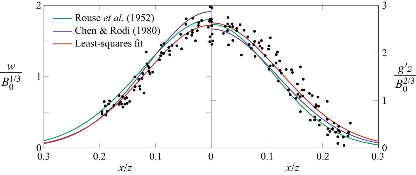
Figure 2. A redrawing of the comparison that Chen & Rodi (Reference Chen and Rodi1980) made between the original fit of Rouse et al. (Reference Rouse, Yih and Humphreys1952) and the revised profiles proposed by Chen & Rodi (Reference Chen and Rodi1980). A least-squares Gaussian fit to the data points is included for comparison.
To assess the appropriateness of either reported fit we have added an (unconstrained) Gaussian least-squares fit to figure 2, which yields the following coefficients:  $C_b=0.167, C_{\lambda b}=0.175, C_w=1.72$ and $C_g=2.63$. While a comparison with the least-squares fit does not definitively show that Chen & Rodi (Reference Chen and Rodi1980) achieved a better fit to the data than Rouse et al. (Reference Rouse, Yih and Humphreys1952), the least-squares fit does support the Chen & Rodi (Reference Chen and Rodi1980) claim that the measurements show $\lambda >1$ ( $C_{\lambda _b}/C_b=1.05$). While the least-squares fit might be expected to be more appropriate than the two constructed fits, this is not true for the purpose of calculating $\alpha$. There are four possible values for $\alpha$ that can be calculated from the least-squares coefficients: $0.148$ ( $C_b$), $0.182$ ${(C_{\lambda b},C_{w})}$, $0.178$ ${(C_{w},C_{g})}$ and $0.079$ ${(C_{\lambda b},C_{g})}$. This poor agreement between values calculated with different pairs is not inevitable – in §§ 4.5 and 4.7 we show that unconstrained Gaussian fits to data can result in a set of values for $\alpha$ in much closer agreement.
We do not include values of  $\alpha$ determined from the Rouse et al. (Reference Rouse, Yih and Humphreys1952) measurements in our curated list (table 4) as there is too much uncertainty regarding which coefficients best represent their measurements. However, the Rouse et al. (Reference Rouse, Yih and Humphreys1952) measurements are important in the historical context, not only as the first of their kind and as revealing the self-similar nature of the profiles, but also because the reported coefficient values influenced the analysis of later measurements, particularly those of Lee & Emmons (Reference Lee and Emmons1961).
4.3. Yokoi (Reference Yokoi1960)
Yokoi (Reference Yokoi1960) measured  $w(x)$ and $g'(x)$ at different heights above a line fire. In his analysis, Yokoi adopts Prandtl's momentum transfer theory (Prandtl Reference Prandtl1925) and Taylor's vorticity transfer theory (Taylor Reference Taylor1932), rather than the framework of the Morton et al. (Reference Morton, Taylor and Turner1956) plume model. With modifications to these theories based on his measurements, Yokoi (Reference Yokoi1960) shows that
 \begin{equation} C_w=1.040 c^{{-}2/9} \quad \mbox{and} \quad C_g=0.663 c^{{-}4/9} , \end{equation}
and obtains  $c^{2/3}=0.13$ from experiment. It would appear that the values $C_w=2.05$ and $C_g=2.6$, and the corresponding values of $\alpha =0.125$ and $\lambda =1.15$, that Yuan & Cox (Reference Yuan and Cox1996) attribute to Yokoi (Reference Yokoi1960) result from (4.1a,b). Yuan & Cox (Reference Yuan and Cox1996) also report that Yokoi (Reference Yokoi1960) ‘explicitly’ measured $\lambda =1.01$. We could not find reference to this, but Yokoi (Reference Yokoi1960) does present plots of velocity and buoyancy profiles. As these plots do not clearly indicate Gaussian-like profiles, we have not attempted to use them to determine $C_b$ or $C_{\lambda b}$, but they do appear to support $\lambda \approx 1.0$ (and not $\lambda =1.15$).
There are difficulties with the interpretation of Yokoi's results, principally, as no clear statement is given as to how  $c$ was measured, or inferred, so judgements concerning its accuracy or precision cannot be readily made. Moreover, the constant $c$ is a component in his analysis using modified transfer theories and non-Gaussian profiles, and it is unclear how this analysis can be reconciled with the Morton et al. (Reference Morton, Taylor and Turner1956) entrainment hypothesis and Gaussian-profile framework adopted here. Although it is unclear how Yokoi (Reference Yokoi1960) interpreted his measurements, we follow Yuan & Cox (Reference Yuan and Cox1996) and use (4.1a,b) to calculate the entries reported for Yokoi (Reference Yokoi1960) in table 3, which are in broad agreement with others. However, we do not include entries for Yokoi's measurements in table 4.
4.4. Lee & Emmons (Reference Lee and Emmons1961)
Lee & Emmons (Reference Lee and Emmons1961) also studied the thermal plume above a line fire. Unlike Rouse et al. (Reference Rouse, Yih and Humphreys1952) and Yokoi (Reference Yokoi1960) they only measured temperature profiles and, consequently, could only determine  $C_{\lambda b}$ and $C_g$. Lee & Emmons (Reference Lee and Emmons1961) present the inverse relations, i.e. $C_g$ and $C_{\lambda b}$ in terms of $\alpha$ and $\lambda$, which can be rearranged to show
 \begin{equation} \alpha =\frac{\sqrt{\rm \pi}C_{\lambda b}}{2}\left(A\pm\sqrt{A^2-1}\right), \quad \lambda =A\mp\sqrt{A^2-1}, \quad \mbox{where } A=\frac{\rm \pi}{\sqrt{2}} C_g^3C_{\lambda b}^2. \end{equation}
The solutions for  $\alpha$ and $\lambda$ in (4.2a,b) share the same basic form and, for a given value of $A>1$, there are clearly two pairs of real-valued solutions. Lee & Emmons (Reference Lee and Emmons1961) report $\alpha =0.16$ and $\lambda =0.9$, which closely align with the values determined from the fits reported by Rouse et al. (Reference Rouse, Yih and Humphreys1952). However, they do not comment on the existence of multiple solutions or the possibility that measurement error could result in non-real-valued solutions.
The solution pair  $\alpha =0.16$ and $\lambda =0.9$ can be calculated to 2 s.f. using $C_{\lambda b}=0.16248$ and $C_g=2.5786$, the latter requiring 5 s.f. in order to achieve the aforementioned precision. This extreme sensitivity is reflected by the large values of the uncertainty multipliers for this pair (table 2). These same coefficient values can be used to calculate a previously unreported second solution pair for which $\lambda >1$, namely, $\alpha =0.13$ and $\lambda =1.1$. It is impossible to select one pair over the other from measurements of the buoyancy profile alone: two different velocity profiles, one ‘faster’ and narrower than the other, each implying different values of $\alpha$ and $\lambda$, could be paired with the buoyancy profile and satisfy the conservation equations. In contrast, a coefficient pair with at least one measurement of the velocity profile does not lead to such an ambiguity. It is unclear if Lee & Emmons (Reference Lee and Emmons1961) deliberately chose the solution branch which agreed more closely with the fits originally reported by Rouse et al. (Reference Rouse, Yih and Humphreys1952) (which erroneously suggested $\lambda <1$) or if they were only aware of the branch chosen. Regardless, the revised fits to the Rouse et al. (Reference Rouse, Yih and Humphreys1952) data (Chen & Rodi Reference Chen and Rodi1980) and all subsequent measurements of $(C_{b},C_{\lambda b})$ (Kotsovinos Reference Kotsovinos1975; Ramaprian & Chandrasekhara Reference Ramaprian and Chandrasekhara1989; Paillat & Kaminski Reference Paillat and Kaminski2014a; Parker et al. Reference Parker, Burridge, Partridge and Linden2020) show $\lambda >1$. Consequently, we consider $\alpha =0.13$ to be the correct interpretation of the Lee & Emmons (Reference Lee and Emmons1961) measurements.
A similar analysis error has propagated in the fire plume literature (e.g. Thomas Reference Thomas1987; Poreh et al. Reference Poreh, Morgan, Marshall and Harrison1998) where, because the transport of smoke is of particular concern, there is emphasis on the coefficient for the variation of volume flux,  $C_Q$, rather than on $\alpha$. Using the framework set out in § 2
 \begin{equation} C_Q=2^{5/6}\alpha^{2/3}(1+\lambda^2)^{1/6}. \end{equation}
Thomas (Reference Thomas1987) used (4.3) to calculate  $C_Q=0.58$ using the original, but seemingly erroneous, values for $\alpha$ and $\lambda$ reported by Lee & Emmons (Reference Lee and Emmons1961). With the revised values for $\alpha$ and $\lambda$ $(>1)$, we obtain $C_Q=0.52$, which is in closer agreement with the other measurements (table 3). Given the potential for ambiguity, we recommend $C_Q$ also be related to the measured quantities directly, viz.
 \begin{equation} C_Q=\frac{1}{C_g}\sqrt{\frac{2A}{A\pm\sqrt{A^2-1}}}, \end{equation}
a form that does not obscure the fact that two solutions are possible. Thomas et al. (Reference Thomas, Morgan and Marshall1998) describe how the excess plume volume flux implied by the values of  $\alpha$ and $\lambda$ originally reported by Lee & Emmons (Reference Lee and Emmons1961) resulted in unnecessarily complex spill plume models used by the Building Research Establishment (BRE) and state that this ‘complexity can be removed by decoupling early BRE work from the experiments of Lee and Emmons’.
A final conclusion concerning the use of the Lee & Emmons (Reference Lee and Emmons1961) data for estimating  $\alpha$ is worthy of mention. The magnitudes of their uncertainty multipliers are $18.1$ ( $C_{\lambda b}$) and $28.7$ ( $C_g$), values that (i) are considerably larger than typical multipliers (table 2) and (ii) render the use of (3.2a) inappropriate. Using (4.2a), we note that if both values of ${(C_{\lambda b},C_{g})}$ were $1\,\%$ smaller then $A<1$ and $\alpha$ could not be determined, but if both values were $1\,\%$ larger then $\alpha$ would reduce from $0.13$ to $0.10$ (both changes being more significant than would be predicted using (3.2a)). Given such sensitivity, the accuracy and precision of their measurements is particularly important but information on this is not provided.
4.4.1. Other measurements of $C_{\lambda b}$ and $C_g$


Harris (Reference Harris1967), Anwar (Reference Anwar1969) and Sangras et al. (Reference Sangras, Dai and Faeth1998) each measured  $g'(x,z)$. However, these measurements have not proven helpful in determining a value for $\alpha$ and are only occasionally cited in this context.
Harris (Reference Harris1967) measured the temperature distribution of a two-dimensional jet of warm water in a cooler freshwater environment. Chen & Rodi (Reference Chen and Rodi1980) attribute values of  $C_g=2.3$ and $C_{\lambda b}=0.163$ to the Harris (Reference Harris1967) measurements (values converted to account for different plume width conventions). We were unable to independently verify these values, primarily because it was unclear which measurements were from regions where the flow was in the far-field equilibrium state of interest. Regardless, this pair of values results in $A=0.718$, and thus (4.2a) cannot be used to determine $\alpha$.
Physically, the condition  $A<1$ implies that the measured Gaussian buoyancy profile does not have a corresponding Gaussian velocity profile which will satisfy the conservation equations (2.2a–c). This condition is widespread and, besides the constrained fits to the Rouse et al. (Reference Rouse, Yih and Humphreys1952) data, only the measurements of Lee & Emmons (Reference Lee and Emmons1961) and Paillat & Kaminski (Reference Paillat and Kaminski2014a) show $A>1$. Other measurements lead to values for $A$ just below one – such as $A=0.85$ (Kotsovinos Reference Kotsovinos1975) and $A=0.95$ (Ramaprian & Chandrasekhara Reference Ramaprian and Chandrasekhara1989) – which could be reasonably attributed to (small) measurement errors. Crucially, these datasets include measurements of other pairs which can be used to determine $\alpha$, and there is no need to rely on the pair ${(C_{\lambda b},C_{g})}$. These measurements of $A<1$ lend credence to the plausible concern that the assumptions underlying plume theory are not always appropriate.
Measurements by both Anwar (Reference Anwar1969) and Sangras et al. (Reference Sangras, Dai and Faeth1998) suffer from the same problem as the Harris (Reference Harris1967) data: the buoyancy profiles show  $A<1$ and no other coefficients are measured. Anwar (Reference Anwar1969) does not explicitly state values for $C_{\lambda b}$ and $C_g$ for his study of freshwater plumes in a saltwater environment, but Chen & Rodi (Reference Chen and Rodi1980) attribute ${C_{\lambda b}=0.156}$ and $C_g=2.57$ to those measurements. This appears to be a fair assessment of the Anwar (Reference Anwar1969) results, and these values yield $A=0.92$. Sangras et al. (Reference Sangras, Dai and Faeth1998) measured the concentration of an iodine tracer in a helium plume in air and determined $C_{\lambda b}=0.120$ and $C_g=2.10$. Their values yield $A=0.30$.
4.5. Kotsovinos (Reference Kotsovinos1975) and Ramaprian & Chandrasekhara (Reference Ramaprian and Chandrasekhara1989)
Both Kotsovinos (Reference Kotsovinos1975) and Ramaprian & Chandrasekhara (Reference Ramaprian and Chandrasekhara1989) measured  $w(x)$ and $g'(x)$ at a number of downstream locations in a thermal plume in water.
It is evident from table 1 that there is a peculiarity regarding the data of Kotsovinos (Reference Kotsovinos1975): Kotsovinos (Reference Kotsovinos1975) reports  $\alpha =0.11$ based on his own measurements of the velocity profile width (2.12a), while Yuan & Cox (Reference Yuan and Cox1996) report $\alpha =0.20$ using (2.13a) and the Kotsovinos (Reference Kotsovinos1975) data for ${(C_{w},C_{g})}$. By contrast, independent assessments of the data of Ramaprian & Chandrasekhara (Reference Ramaprian and Chandrasekhara1989) yield only marginal variations in $\alpha$: Ramaprian & Chandrasekhara (Reference Ramaprian and Chandrasekhara1989) determined $\alpha =0.113$ from their own measurements of ${(C_{w},C_{Q})}$, while calculations by Yuan & Cox (Reference Yuan and Cox1996), using ${(C_{w},C_{g})}$, and Paillat & Kaminski (Reference Paillat and Kaminski2014a), using $C_b$, both concluded $\alpha =0.117$.
In general, it is not surprising that different coefficient pairs should lead to marginally different values for  $\alpha$ on account of small errors in measurement or in the fitting of Gaussian profiles to determine $C_{b}, C_{\lambda b}, C_w$ and $C_g$. The least-squares fit to the Rouse et al. (Reference Rouse, Yih and Humphreys1952) data highlighted the challenge in achieving a consistent set of values for $\alpha$ determined from different pairs. However, the difference between $\alpha =0.11$ and $\alpha =0.20$ cannot be simply explained by a small error and suggests that the measurements made by Kotsovinos (Reference Kotsovinos1975) are not self-consistent.
Chen & Rodi (Reference Chen and Rodi1980), Ramaprian & Chandrasekhara (Reference Ramaprian and Chandrasekhara1989) and Parker et al. (Reference Parker, Burridge, Partridge and Linden2020) have all cast doubt on some aspects of the Kotsovinos (Reference Kotsovinos1975) measurements, and it seems likely that the Kotsovinos (Reference Kotsovinos1975) value of  $C_w$ is erroneous. Consequently, we reject the value $\alpha =0.20$ calculated by Yuan & Cox (Reference Yuan and Cox1996). Looking beyond $C_w$, we could not identify any specific reason that the widths of the velocity and scalar profiles would be incorrect, and the values of $\alpha =0.10$ and $\lambda =1.28$ that result from the pair $(C_{b},C_{\lambda b})$ are not unreasonable. These values are slightly different to those usually attributed to Kotsovinos (Reference Kotsovinos1975), as explained in Appendix C.
The values of the measurements reported by Ramaprian & Chandrasekhara (Reference Ramaprian and Chandrasekhara1989) are in good agreement with others (table 3), and are seemingly self-consistent given the close similarities in the independently calculated values of  $\alpha$. We further demonstrate the self-consistency in § 4.7 where we attribute the value $\alpha =0.115$ to their dataset. However, some aspects of their dataset raise concern. They report on only four experiments, including one where the plume buoyancy flux drops by over $50\,\%$ in their measurement region. The small number of experiments is concerning as the (unreported) variation of the value of $C_Q$ in individual experiments exceeds $10\,\%$.
4.6. Yuan & Cox (Reference Yuan and Cox1996)
The approach of Yuan & Cox (Reference Yuan and Cox1996) is an exemplar of the application of plume theory in the design of experiments. They showed that measuring only the centreline properties, rather than entire plume profile(s), is sufficient to deduce  $\alpha$. Although they could not then show the self-similarity of cross-stream profiles, they confirm that their measurements were of a fully developed line plume by showing that their centreline measurements followed the power laws $g_c'\propto B_0^{2/3}z^{-1}$ and $w_c\propto B_0^{1/3}z^0$. Their measurements of volume flux using the hood method (Zukoski et al. Reference Zukoski, Kubota and Cetegen1981), while not as comprehensive, were complementary and the measured value of $C_Q=0.51$ is in good agreement with the value $C_Q=0.48$ which they calculated using their values of ${(C_{w},C_{g})}$ (table 3). Yuan & Cox (Reference Yuan and Cox1996) do not report any uncertainties for their measurements, but their well-populated plots of centreline temperature and velocity show minimal scatter.
4.7. Paillat & Kaminski (Reference Paillat and Kaminski2014a) and Parker et al. (Reference Parker, Burridge, Partridge and Linden2020)
Paillat & Kaminski (Reference Paillat and Kaminski2014a) and Parker et al. (Reference Parker, Burridge, Partridge and Linden2020) measured  $w(x,z)$ and $g'(x,z)$ in the central plane of a saline plume using particle image velocimetry and laser induced fluorescence. Paillat & Kaminski (Reference Paillat and Kaminski2014a) report values of $\alpha$ and $\lambda$ calculated using $(C_{b},C_{\lambda b})$. While values for $(C_w,C_g)$ are not reported, $C_w\approx 2.1 - 2.2$ and $C_g\approx 2.8 - 2.9$ can be read from their plots and are listed in table 3 as the mid-range values: $C_w=2.15$ and $C_g=2.85$.
Parker et al. (Reference Parker, Burridge, Partridge and Linden2020) report  $\alpha _T=0.14$ for the top-hat entrainment coefficient, which corresponds to $\alpha =0.10$ (approximately). While they do not report values for the coefficients $C_b, C_{\lambda b}, C_w, C_g$ or $C_M$, our analysis of the data they provide allows these coefficients to be estimated (Appendix D). Values resulting from this analysis are included in table 3.
The three sets of entries in table 3 for Parker et al. (Reference Parker, Burridge, Partridge and Linden2020) account for the three different representative buoyancy fluxes that we used to normalise their profile measurements: the source buoyancy flux  $B_{0,S}$ (determined from the volume flux and buoyancy of the source fluid), the mean buoyancy flux $B_{0,M}$ measured in the plume and the total buoyancy flux $B_{0,T}$ measured in the plume (determined as the sum of the mean and turbulent components). Classic plume theory assumes that the turbulent component is relatively small, and, thus, $B_{0,S}\approx B_{0,M} \approx B_{0,T}$. However, Parker et al. (Reference Parker, Burridge, Partridge and Linden2020) measured, on average, $B_{0,M}=0.84B_{0,S}$ and $B_{0,T}=0.94B_{0,S}$, and normalising their measurements by these buoyancy fluxes results in differences in coefficient values of similar magnitude to the differences between the other experimental campaigns (table 3). There is no obvious consensus from past campaigns on the ‘most’ representative buoyancy flux as all three have been used – Rouse et al. (Reference Rouse, Yih and Humphreys1952) normalise using the mean, Ramaprian & Chandrasekhara (Reference Ramaprian and Chandrasekhara1989) normalise with the total and Lee & Emmons (Reference Lee and Emmons1961) normalise with the source buoyancy flux – although these choices are, in part, a result of experimental capabilities.
Based on the coefficient values we have determined from the data of Paillat & Kaminski (Reference Paillat and Kaminski2014a) and Parker et al. (Reference Parker, Burridge, Partridge and Linden2020),  $\alpha$ may now be estimated in multiple ways, a selection of which are plotted in figure 3. To aid wider comparisons, also plotted are the values for $\alpha$ determined from (i) the measurements of $\alpha _T$ by Parker et al. (Reference Parker, Burridge, Partridge and Linden2020), (ii) from the dataset of Ramaprian & Chandrasekhara (Reference Ramaprian and Chandrasekhara1989), where we have normalised the measurements by $B_{0,M}$ in Appendix E, and (iii) from our own measurements (§ 5).

Figure 3. Values of  $\alpha$ calculated from coefficient pairs or $\alpha _T$. Error bars show $95\,\%$ confidence intervals calculated with (3.2a), for pairs where the confidence interval for the measurements could be determined. Note: PBPL (Parker et al. Reference Parker, Burridge, Partridge and Linden2020), PK (Paillat & Kaminski Reference Paillat and Kaminski2014a), RC (Ramaprian & Chandrasekhara Reference Ramaprian and Chandrasekhara1989).
Amidst the range of values of  $\alpha$ in figure 3, we can highlight four key results. First, for a dataset where at least three coefficients are measured it is potentially misleading to report a single value for $\alpha$ (i.e. as determined from a single coefficient pair) given a different coefficient pairing could lead to a significantly different value for $\alpha$. While the value $\alpha =0.113$ reported by Ramaprian & Chandrasekhara (Reference Ramaprian and Chandrasekhara1989) using the pair ${(C_{w},C_{Q})}$ is the median value of the seven values calculated for their data, the value $\alpha =0.126$ reported by Paillat & Kaminski (Reference Paillat and Kaminski2014a) using $C_b$ is the highest of the three values for theirs.
Second, the choice of normalisation (by  $B_{0,S}, B_{0,M}$ or $B_{0,T}$) only impacts certain coefficient pairs. As would be expected, there is no impact if $\alpha$ is determined from $C_b$, where only the velocity profile width matters, or from the pairs ${(C_{w},C_{Q})}$ and ${(C_{Q},C_{M})}$, where the buoyancy flux ‘cancels out’. However, for other pairings such as ${(C_{w},C_{g})}$ or ${(C_{g},C_{Q})}$ the difference can be significant. Intriguingly, normalising the Parker et al. (Reference Parker, Burridge, Partridge and Linden2020) measurements by $B_{0,M}$ results in very consistent values for $\alpha$, with an absolute difference of only $0.005$ between the largest and smallest value. This consistency is perhaps unsurprising given that only the mean buoyancy flux is considered in classic plume theory and van Reeuwijk et al. (Reference van Reeuwijk, Salizzoni, Hunt and Craske2016) reached a similar conclusion with their direct numerical simulation data for axisymmetric plumes. Normalisation with $B_{0,M}$ did not result in a more consistent set using the Ramaprian & Chandrasekhara (Reference Ramaprian and Chandrasekhara1989) data, although there are concerns with the dataset (§ 4.5).
Third, while selecting a single value for  $\alpha$ to represent each dataset is not necessarily trivial, the median of the plotted values yields the following representative values (rounded to the nearest $0.005$): $\alpha =0.095$ (Parker et al. Reference Parker, Burridge, Partridge and Linden2020), $\alpha =0.115$ (Ramaprian & Chandrasekhara Reference Ramaprian and Chandrasekhara1989) and $\alpha =0.120$ (Paillat & Kaminski Reference Paillat and Kaminski2014a). The rounded values for Ramaprian & Chandrasekhara (Reference Ramaprian and Chandrasekhara1989) and Parker et al. (Reference Parker, Burridge, Partridge and Linden2020) are the same for each ‘set’ of coefficient measurements, irrespective of the normalising buoyancy flux.
Fourth, the  $95\,\%$ confidence intervals for the Parker et al. (Reference Parker, Burridge, Partridge and Linden2020) measurements span a considerable range of values for $\alpha$, and the size of the interval varies with the coefficient pairing. The smallest interval is $\pm 6\,\%$ for $(C_{\lambda b},C_{w})$ when the measurements are normalised by the mean or total buoyancy flux. From the standard deviation of $\pm 7\,\%$ that Paillat & Kaminski (Reference Paillat and Kaminski2014a) reported for $C_b$ (based on measurements from ten experiments), we calculate a confidence interval of $\pm 5\,\%$. The $\pm 2\,\%$ interval determined from our experiments (§ 5) compares favourably with these past measurements.
Figure 3 also shows the link between  $\alpha$ calculated using the pair ${(C_{Q},C_{M})}$ and based on $\alpha _T=\mathrm {d} (Q^2/M)/ \mathrm {d} z$, as the values determined from these two approaches using the data of Parker et al. (Reference Parker, Burridge, Partridge and Linden2020) are almost identical. While this agreement is not surprising given the dual reliance on the measurements of the volume and momentum flux, the difference in the confidence intervals calculated using either approach highlights that care should be taken when evaluating the uncertainty in an experiment or a particular pair. In this case, where $Q$ and $M$ are determined from the same velocity profile and thus correlated, the approach described in § 3 may not be the most appropriate; the narrower confidence intervals around the value determined from $\alpha _T$ are likely better reflections of the precision achieved when using measurements of the volume and momentum flux.
The range of values for  $\lambda$ calculated from different coefficient pairings (figure 4) can be analysed in a similar manner, and we only highlight the following points herein. The variation in the individual values for $\lambda$, and the extent of the confidence intervals, is larger than for $\alpha$, although this is not surprising given the larger uncertainty multipliers for $\lambda$ (table 2). The representative values reported in table 4 for these datasets were determined in a similar manner to $\alpha$: determining the median values and rounding to the nearest $0.05$.
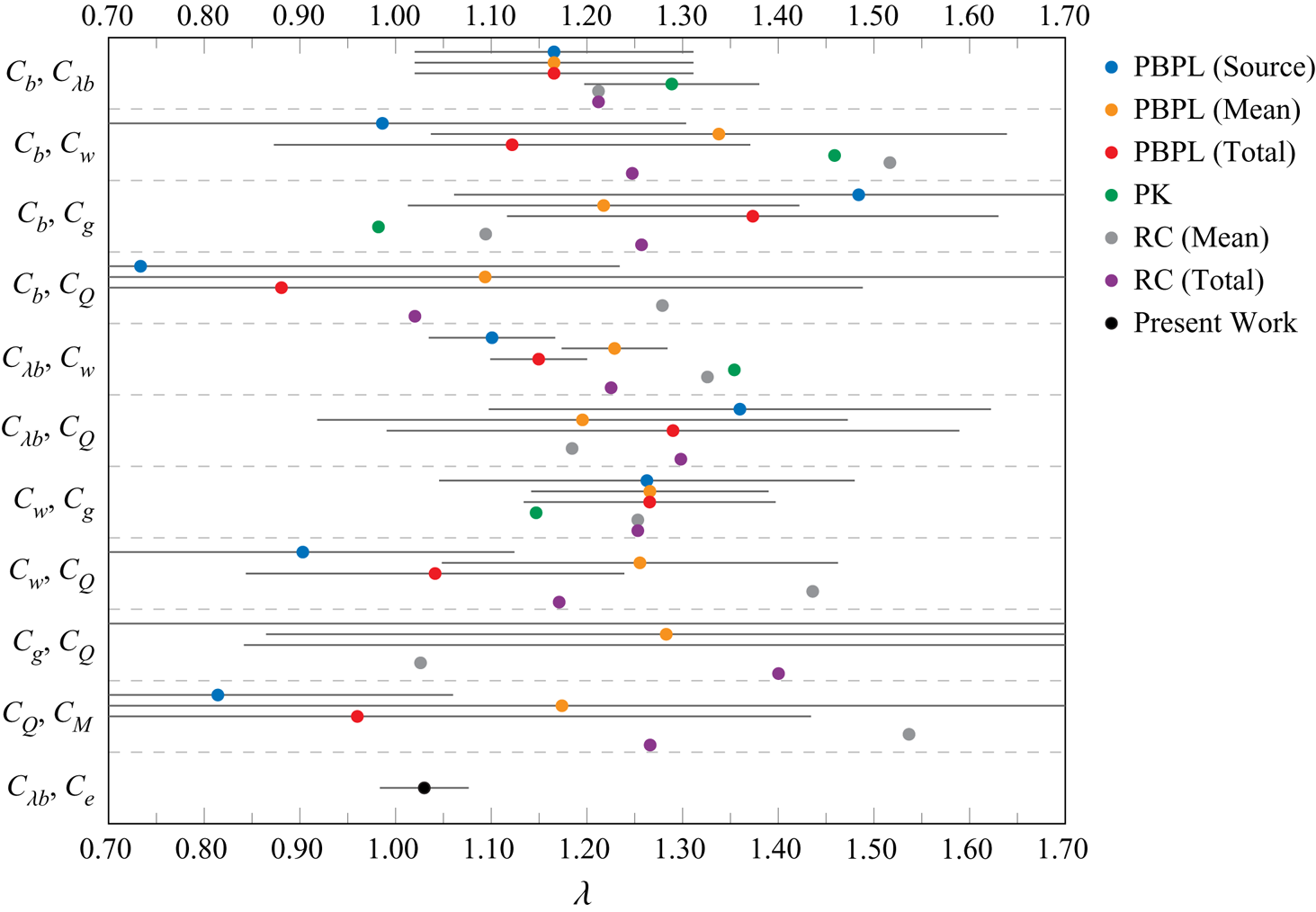
Figure 4. Values of  $\lambda$ calculated using different coefficient pairs. Error bars show $95\,\%$ confidence intervals for $\lambda$ calculated using (3.2b), for pairs where the confidence interval for the measurements could be determined. Note: PBPL (Parker et al. Reference Parker, Burridge, Partridge and Linden2020), PK (Paillat & Kaminski Reference Paillat and Kaminski2014a), RC (Ramaprian & Chandrasekhara Reference Ramaprian and Chandrasekhara1989).
4.8. Summary of the analysis of the experimental literature
The primary objective of the preceding analysis was to determine the underlying reasons for the wide variation in the reported values for  $\alpha$, which we achieved by reasoning why three of the largest reported values for $\alpha$ are not appropriate. While doubts about aspects of the experiments of Rouse et al. (Reference Rouse, Yih and Humphreys1952), Lee & Emmons (Reference Lee and Emmons1961) and Kotsovinos (Reference Kotsovinos1975) have been previously raised, we believe we are the first to identify that an alternate value of $\alpha$ can be calculated from the Lee & Emmons (Reference Lee and Emmons1961) measurements. In addition, using the measurements of Ramaprian & Chandrasekhara (Reference Ramaprian and Chandrasekhara1989) and Parker et al. (Reference Parker, Burridge, Partridge and Linden2020) we showed that the theoretical extension to determine $\alpha$ from a multitude of coefficient pairings was appropriate, as the many calculated values were broadly in agreement, allowing for uncertainty (figure 3). By considering multiple pairs, we also determined a single representative value of $\alpha$ for each of the datasets reported by Ramaprian & Chandrasekhara (Reference Ramaprian and Chandrasekhara1989), Paillat & Kaminski (Reference Paillat and Kaminski2014a) and Parker et al. (Reference Parker, Burridge, Partridge and Linden2020). Table 4 is the culmination of our analysis and contains a curated list of values which we have reasoned represents the spread in the values of $\alpha$. The range $0.095\lesssim \alpha \lesssim 0.13$ is narrower than $0.10\lesssim \alpha \lesssim 0.20$, and more appropriately represents the uncertainty surrounding $\alpha$. Also summarised therein are the values of $\lambda$ determined from these datasets, and we consider $\lambda =1.2$ (average value, rounded to 2 s.f.) to be the representative value.
5. A new measurement approach to determine the entrainment coefficient
Our analysis (§§ 2–4) has reduced the range of  $\alpha$, arguably by about $70\,\%$. Rather than merely to add to the small array of previously published measurements, a set-up was designed and a programme of experiments conceived with the specific goal of determining $\alpha$ to a greater precision. To this end, we took a previously unconsidered measurement approach and made measurements of a greater number of plumes than in other recent experimental campaigns. In this way, we were able to better account for the inherent variability in turbulent plumes, and determine $\alpha$ with a confidence interval smaller than was achieved with past experiments.
While some pairings carry a lower uncertainty, there is no obvious pairing of coefficients that should be targeted (§§ 2–3). Given the definition of  $\alpha$ (1.1), an approach conceived to measure the entrainment velocity $u_e$ directly would appear to be a natural choice. Although observations of plume-induced flows have been made (Harris Reference Harris1967; Kotsovinos Reference Kotsovinos1975), we found no published reports of $\alpha$ determined from measurement of $u_e$. To complete the pair and thereby estimate $\alpha$, we sought to measure the width of the scalar profile $C_{\lambda b}$, as this coefficient has the smallest uncertainty multiplier when paired with $C_e$ (table 2a). For completeness, $\lambda$ was also estimated using this pair.
5.1. General set-up and approach
Experiments to determine both  $C_e$ and $C_{\lambda b}$ were initiated by steadily releasing a sodium chloride solution from a slender rectangular source into a freshwater-filled clear acrylic visualisation tank of horizontal dimensions $2770~\textrm {mm} \times 250~\textrm {mm}$ and vertical dimension 500 mm. After accounting for residual temperature differences between the freshwater and saline solution, the source density difference was determined to within $1\,\%$ using an Anton Paar 5000M densitometer.
The source was a slot of length  $L=220$ mm machined in the lower face of a bespoke constant head tank, centred in the visualisation tank and supported 400 mm above the base. Using digital callipers, the width of the slot ( $s=2b_0$) was measured as $3.00\pm 0.15$ mm at ten points along its length, giving $L/s = 73.3$. Besides the $15$ mm wall thickness at either end, the source spanned the entire $250$ mm dimension of the visualisation tank. The constant head tank was supplied with saline solution using an Ismatec MCP-Z Process gear pump. Near uniform conditions were produced along the full length of the slot as shown in figure 5. While the majority of the experiments considered the central plane of the visualisation tank ( $y=0$), ten experiments involved measurements at $y\approx 0.25 L$ to verify the two-dimensionality of the flow field. The source flow rate $Q_0$ (cm $^{2}$ s $^{-1}$) was determined by tracking the free surface in the constant head tank (horizontal dimensions $486 \pm 1$ mm by $200\pm 1$ mm). Recording the vertical position of the free surface at three frames per second (f.p.s.) and a resolution of 20 pixels per cm (approximately), $Q_0$ was determined to within $1\,\%$. Table 5 reports the mean flow rate during an experiment and the largest deviation from the mean (typically less than $2\,\%$).
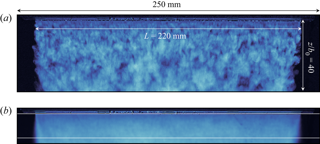
Figure 5. Images of the span of the plume ( $y$–
$y$– $z$ plane). (a) An instantaneous snapshot showing that the flow appears uniform and turbulent along the length $L$ of the source. (b) A time-averaged image of the near-source region showing the horizontally integrated dye concentration, a proxy for the amount of dye introduced from the source. Averaged vertically between the indicated depths ( $z/b_0\approx 1$ and $z/b_0\approx 10$), the concentration varies from the mean by $10\,\%$ over the central $90\,\%$ of the span and by only $5\,\%$ over the central $50\,\%$.
Table 5. Experimental parameters and measurements for the 32 entrainment coefficient experiments. The distance  $z_p$ is an estimate of the distance required for the plume to adjust from its source condition, as characterised by the Richardson number $\varGamma _0$, to ‘pure-like’ behaviour. The values of $\alpha$ and $\lambda$ for an individual experiment are calculated via (5.3a,b). The percentage uncertainties are described in the main text: $Q_0, g'_0$ and $B_0$ (§ 5.1); $C_e$ (§ 5.2) and $C_{\lambda b}$ (§ 5.3). In the starred experiments, measurements of $C_e$ were conducted at $y\approx 0.25 L$ rather than in the central plane of the visualisation tank.
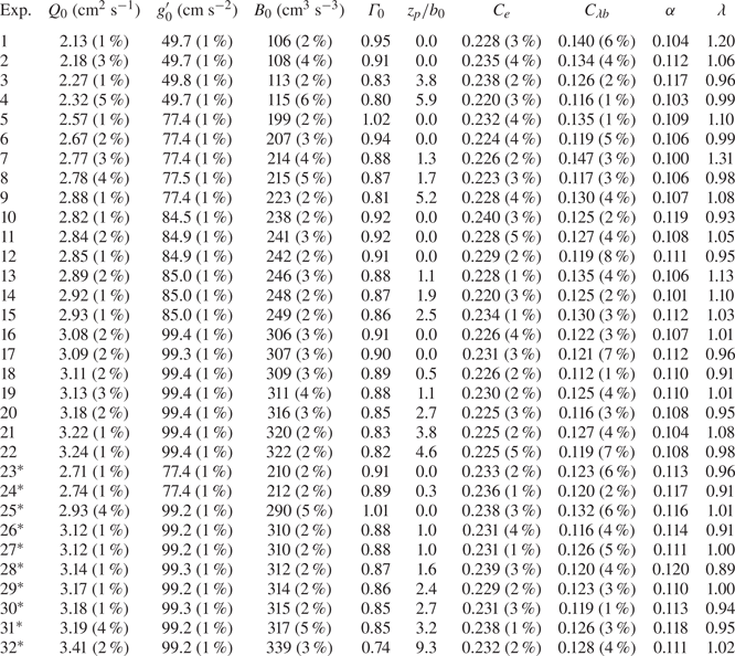
We conservatively report the uncertainty in the source buoyancy flux ( $B_0=Q_0g'_0$) as the sum of the uncertainties in $Q_0$ and $g'_0$. As $C_e$ is calculated by normalising measurements of $u_e$ by $B_0^{1/3}$, the uncertainty in $B_0$ typically affects the values of $C_e$ by less than $1\,\%$, and by $2\,\%$ in the worst case. This variation resulting from the uncertainty in the source conditions is significantly smaller than the actual variation in the measurement of $u_e$ (§ 5.2).
The entrainment velocity and scalar width were determined from a set of 32 experiments, the details of which are summarised in table 5. The source flow rate  $Q_0$ and reduced gravity $g'_0$ were selected to approximate the dynamical conditions of a pure turbulent plume. The source Reynolds number $Re_0$ is the ratio of $Q_0$ to the kinematic viscosity of the source fluid; typically $Re_0=200 - 300$. How ‘pure like’ the release was at source was characterised using the scaled source Richardson number $\varGamma _0$, where $\varGamma _0=1$ indicates a pure plume (van den Bremer & Hunt Reference van den Bremer and Hunt2014a). Assuming top-hat profiles at the source, as is reasonable for the high Reynolds number release conditions,
 \begin{equation} \varGamma_0=2^{3/2}\frac{b_0^3g'_0}{\alpha Q_0^2}. \end{equation}
The entries for  $\varGamma _0$ in table 5, based on $\alpha =0.11$, confirm that the plumes were nominally pure at source. Moreover, using the van den Bremer & Hunt (Reference van den Bremer and Hunt2014a) solutions for an area source plume, the downstream distance $z_p$ over which the Richardson number adjusts from the value at source to within $10\,\%$ of $\varGamma =1$ was estimated to be $z_p/b_0\approx 0 - 10$, while the measurement region of $65 \lesssim z_m/b_0 \lesssim 130$ was considerably further downstream. Given $z_m \gg z_p$ our measurements were recorded within the pure-plume equilibrium region.
The visualisation tank was backlit with a white LED panel and images of the flow recorded at a frame rate of  $12.5$ f.p.s. using a 5 mega-pixel monochrome camera (JAI SP-5000M-USB) with a $75$ mm fixed focal length lens (Kowa Optimed) and a $660$ nm bandpass filter (Midwest Optical Systems). The spatial resolution was $42$ pixels per cm (approximately). Figure 6 shows an image taken from one experiment, annotated to indicate the regions where the plume width and entrainment velocity were measured. The representative length scale $b_r$, defined as the average scalar half-width at the midpoint of the measurement region (estimated using our measured value $C_{\lambda b}=0.126$), and used as a reference for interpretation of the measurements of $C_e$, is also shown. Details specific to the measurement of $C_e$ and $C_{\lambda b}$ are discussed in §§ 5.2 and 5.3, respectively.
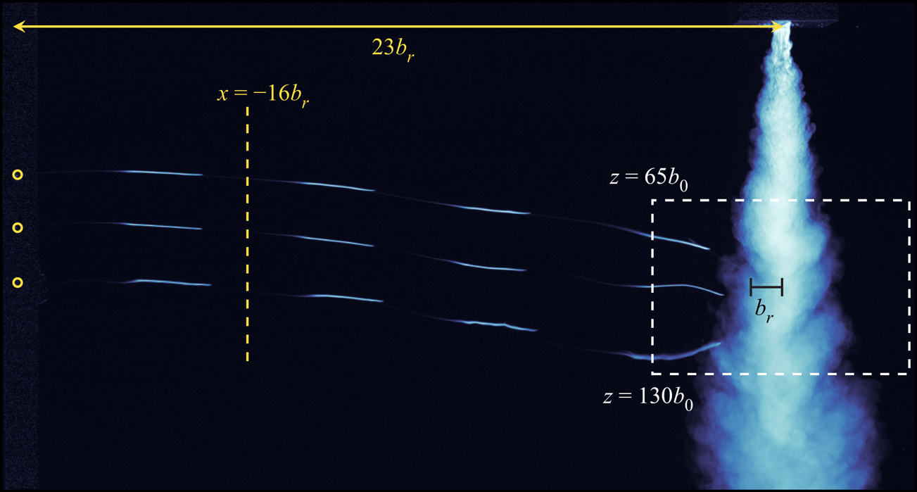
Figure 6. Instantaneous image of a saline plume and its induced-flow field. The entrainment coefficient was determined from combined measurements of: (i) the average velocity of dyeline segments for  ${x \in -[16b_r,5b_r]}$ (approximately) and (ii) the plume scalar width in the region bounded by the dashed white outline. The representative length scale $b_r$ is the plume half-width evaluated at the midpoint of the measurement region ( $z=97.5b_0$). Circles at $x=-23b_r$ indicate the sources of the dyelines.
5.2. Measurement of $C_e$

The velocity  $u_e$ was determined by tracking six dyeline segments per experiment in the induced-flow field. The dyelines emerged at three depths from hypodermic needles (figure 6) connected to a syringe pump programmed to dispense laminar pulses of dyed freshwater (density within $0.01\,\%$ of the environment). Needles of different length were used to release dyelines at $y=0$ (Exps. 1–22) or at $y=56$ mm (Exps. 23–32). The horizontal position of the leading edge of each segment was tracked from $x/b_r=-16$ until the segment was distorted by turbulent fluctuations, which typically occurred $2b_r - 4b_r$ from the plume centreline; $90\,\%$ of the segments were tracked for at least $10b_r$, a distance large relative to the plume width. A typical segment covered this distance ( $\sim 21$ cm, $\sim 900$ pixels) in 200 frames ( $\sim 16$ s) and thus the velocity of each segment, determined from the gradient of a least-squares linear fit to the position-against-time data (figure 7a) was well resolved. Given the spatial uniformity of the predicted induced-flow field (Taylor Reference Taylor1958), the variation in the velocity of the segments was expected to be small. This was indeed the case, with the relative standard deviation being only $3\,\%$ of the average velocity for the six segments shown in figure 7. Similarly small variations were recorded for the segments tracked during Exp. 1 through to Exp. 32 (table 5).
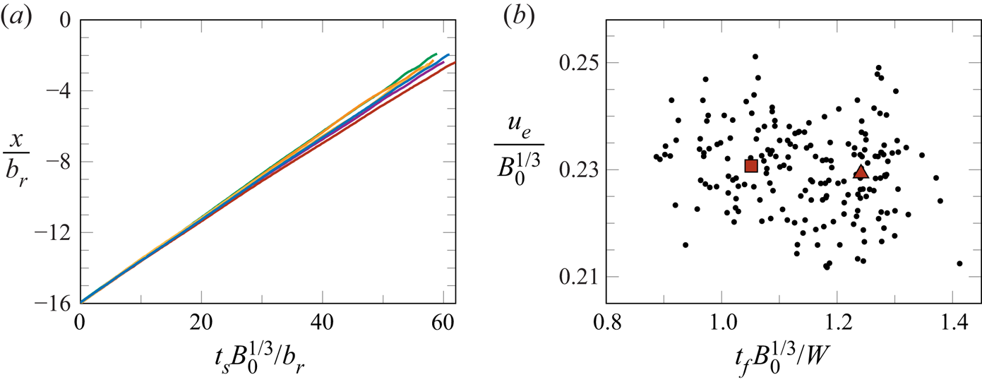
Figure 7. (a) Dimensionless position  $x/b_r$ of the leading edge of six dyeline segments against time $t_s B_0^{1/3}/b_r$ from Exp. 17. The time origin $t_s=0$ was taken as the first frame where the leading edge of a segment crossed the ‘start’ line at $x/b_r=-16$. (b) Entrainment velocity $u_e/B_0^{1/3}$ against measurement time $t_fB_0^{1/3}/W$, where $W$ (
$W$ ( $=2770$ mm) is the tank width, for all 192 segments measured to determine $C_e$ (Pearson's correlation coefficient of $-0.18$. The $p$-value is $0.01$ and the null hypothesis of no correlation is rejected at the $5\,\%$ significance level). Ensemble average velocity and measurement time for the first ( $\blacksquare$) and second ( $\blacktriangle$) waves of 96 segments.
Tracking occurred during the quasi-steady period after the starting plume vortex had passed and before the measurement region filled with buoyant fluid. To assess whether the measured velocities were influenced by filling-box effects, the leading edge of two consecutive ‘waves’ of segments were tracked. Figure 7(b) plots the normalised velocity for each segment against the mean time that that measurement was made. The time origin  $t_f=0$ corresponds to the instant the plume source was activated. Averaged over 96 segments released in the first wave, $C_e=0.231$ while $C_e=0.229$ over the second. The difference is small relative to the overall scatter in the measurements, and both values fall within the confidence interval we report for $C_e$. Thus, we conclude that the entrainment velocity was not significantly impacted by any transient filling behaviour.
5.3. Measurement of $C_{\lambda b}$

Measurements of the light attenuated by methylene blue dye mixed into the source fluid were used to infer the salt concentration in the plume (Cenedese & Dalziel Reference Cenedese and Dalziel1998; Allgayer & Hunt Reference Allgayer and Hunt2012). The time-averaged concentration field and the corresponding buoyancy profiles from a typical experiment are shown in figure 8(a,b), respectively. The concentration field has a resolution of 407 pixels (vertical) by 600 pixels (horizontal) and is an average of 200 frames recorded over  $\tau _a=16$ s. The averaging time $\tau _a$ represents the available measuring time, which was limited primarily by the physical scale of the visualisation tank. Importantly, $\tau _a$ was large relative to two physical time scales $(\tau _e,\tau _t)$ that characterise the flow, namely, the time scale associated with a typical eddy $\tau _e$ (a turnover time) and the time scale required for a notional eddy to traverse the vertical extent ( $\sim 65b_0$) of the measurement window $\tau _t$. Using the centreline velocity as the representative velocity scale, we define
 \begin{equation} \tau_e=\frac{2C_{\lambda b} z_m}{C_wB_0^{1/3}} \quad \mbox{and} \quad \tau_t=\frac{65b_0}{C_wB_0^{1/3}}, \end{equation}
and take  $C_w=2.157$ (i.e. the value used to estimate the uncertainty multipliers (§ 3)) and $C_{\lambda b}=0.126$ from our measurements. Based on the source conditions (table 5), ${\tau _e \approx 0.16 - 0.48 ~\mathrm {s}}$ and so we expect that 30 to 100 ‘eddies’ would form at a particular depth in the interrogation window during the averaging period. Moreover, $\tau _t \approx 0.65 - 0.96$ s and, thus, we expect between 16 and 25 ‘cycles’ where plume fluid traversing the measurement window is entirely refreshed. Given $\tau _a/\tau _e \gg 1$ and $\tau _a/\tau _t \gg 1$, and the Gaussian-like concentration profiles in figure 8(b), we conclude that our measurements appropriately capture a time-averaged line plume.
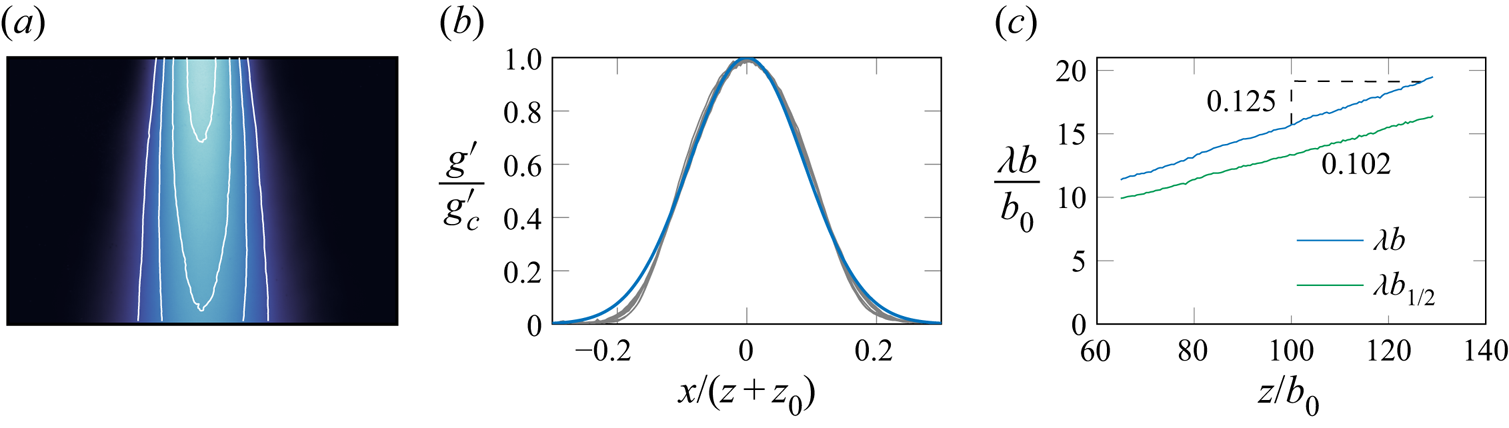
Figure 8. (a) Time-averaged image of the plume in the measurement window for Exp. 14 showing the expected ‘cigar-shaped’ contours of constant buoyancy. (b) In grey, time-averaged dimensionless buoyancy profiles recorded at ten different heights in the plume. In blue, a Gaussian fit calculated using the value  $C_{\lambda b}=0.125$ measured in Exp. 14 shows the Gaussian model is appropriate. The virtual origin $z_0$ was determined by extrapolating the variation of the $1/e$ scalar width with depth to zero width. (c) The half-width of the buoyancy profile using the $g'/g'_c=1/e$ and $g'/g'_c=1/2$ thresholds.
Figure 8(c) shows the variation of  $\lambda b$ and the half-maximum half-width $\lambda b_{1/2}$, i.e. the horizontal distance from the centreline to the point where $g'=0.5g'_c$. The gradient of the $\lambda b$ line, determined using a least-squares linear fit, gives $C_{\lambda b}$. For a Gaussian profile, the ratio of the half-widths $r_G=\lambda b_{1/2}/\lambda b=\sqrt {\ln 2}\approx 0.83$; for the buoyancy profile shown in figure 8(c), this measured ratio is $r_M=0.81$. Averaged across the 32 experiments, we measured $r_M=0.80$, which is within $4\,\%$ of the expected Gaussian value. The ratio of these widths is used to give an indication of the uncertainty in the measurements of $C_{\lambda b}$, and the reported uncertainty estimates in table 5 are values of $|1-r_M/r_G|$.
5.4. Overall results
Our measurements of  $C_e$ and $C_{\lambda b}$ from the 32 experiments are plotted in figure 9. Figures 9(a) and 9(b) indicate the mean values and variation of the measurements. Figure 9(c) shows that the variation in $C_{\lambda b}$ is not correlated with the variation in $C_e$, and thus we conclude that it is reasonable to apply the analysis from § 3 to determine the uncertainty in $\alpha$ and $\lambda$. Following the framework established in § 2, our estimates for $\alpha$ and $\lambda$ are
 \begin{equation} \alpha=C_e^{3/2}\sqrt{\frac{\sqrt{2A^2+1}-1}{A}}, \quad \lambda =\sqrt{\frac{2}{\sqrt{2A^2+1}-1}}, \end{equation}
where  $A=8C_e^3/({\rm \pi} C_{\lambda b}^2)$. The associated uncertainty multipliers are given in Appendix A.
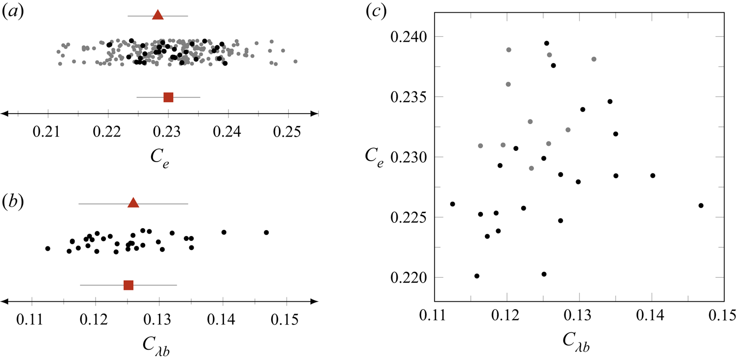
Figure 9. (a) Values of  $C_e$. (b) Values of $C_{\lambda b}$. In (a), in grey, values for every individual dyeline segment ( $6 \times 32$ dots). In (a,b), $\bullet$ average value for each of the 32 experiments; $\blacktriangle$ average value and standard deviation across the centred dyeline experiments; $\blacksquare$ average value and standard deviation across all 32 experiments. (c) Value of $C_e$ against $C_{\lambda b}$ for each of the 32 experiments, grey dots denote an off-centred dyeline experiment; the scatter indicates there is no clear correlation between the two quantities (Pearson's correlation coefficient of $0.19$. The $p$-value is $0.29$ so the null hypothesis of no correlation is not rejected at the $5\,\%$ significance level).
Table 6. The entrainment coefficient  $\alpha$ and profile coefficient $\lambda$ determined in the present study from measurements of $C_e$ and $C_{\lambda b}$. The values of the standard deviation (SD) and the $95\,\%$ confidence interval (CI) for $\alpha$ and $\lambda$ were calculated using the corresponding values in the measurements and the uncertainty multipliers for the pair (A9a,b). Results are shown as a summary of all experiments and of the subsets categorised by dyeline position.
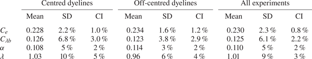
Table 6 summarises the experimental data and the calculated values for  $\alpha$ and $\lambda$ for all the experiments and for the centred and off-centred subsets. There are small differences between measurements depending on the dyeline location. As $C_{\lambda b}$ is determined from measurements of light attenuation through the length of the plume, the mean value of $C_{\lambda b}$ should be unaffected by the dyeline position; the $2\,\%$ difference between the centred and off-centred subsets is attributed to random variation. The mean $C_e$ values measured at each dyeline needle position are within $3\,\%$ of each other, and this similarity supports the claim that the flow field is approximately two-dimensional. The small difference between the mean $C_e$ values may result from the effects of the end walls, small variations in the conditions along the plume source or random variation. The difference in the values of $\alpha$ and $\lambda$ determined from all experiments or from only the centred experiments is small compared with the variation between other reported values (table 4). In the absence of a detailed study of the variations along the span of a line plume, only the measurements from the experiments with centred dyelines were used to determine the key result: $\alpha =0.108$ with a $95\,\%$ confidence interval of $2\,\%$.
6. Discussion
Our experimental campaign successfully demonstrated that the entrainment velocity can be accurately measured and used to determine the entrainment coefficient. The resulting value of  $\alpha =0.108$ is very similar to the average value of the curated datasets following the literature analysis ( $\alpha =0.114$), and is bounded by a narrower confidence interval than past values for $\alpha$. The narrower interval arises from two factors: the variation in the measurements (i.e. the standard deviation) is less than or comparable to the variation reported in other datasets and the number of experiments is greater.
Although we did not set out to determine  $\lambda$ – and would have chosen a different experimental approach if $\lambda$ were the target – we calculate that $\lambda =1.03$. While lower than the other values in table 4, this value is within $20\,\%$ of the representative value $\lambda =1.2$. A difference of this magnitude is typical for calculated values of $\lambda$ (figure 4) and is unsurprising on both experimental and theoretical grounds. The considerable variation in past measurements of $C_{\lambda b}$ (table 3) suggests that the plume width is sensitive to small changes in experimental conditions or is difficult to measure. On theoretical grounds, we discussed how turbulent fluxes have a small but non-negligible impact (§ 4.7) and showed that the scalar profile is only approximately Gaussian (§ 5.2), both factors which could influence the accuracy of calculations made using plume theory. In this context, the agreement between our calculated value and values determined directly from measurements of the plume widths is reassuring.
It is intriguing that there is considerable variation in the measurements across the experiments, with the most extreme values for  $C_{\lambda b}$ approximately $17\,\%$ different to the mean and $5\,\%$ different for $C_e$. This variation is broadly comparable to variations observed in past experiments, and although we were unable to link it to any particular aspect of the experimental set-up or measurement process, it seems possible that some of the variation between experiments would reduce if the time-averages were far longer. In their study of line jets, Paillat & Kaminski (Reference Paillat and Kaminski2014b) attribute variations in their entrainment measurements to turbulence effects which occur at lower Reynolds numbers. Comparisons between jet and plume behaviour are not necessarily straightforward, but in light of their measurements (and, as far as we are aware, the absence of a similar study specific to line plumes), it seems reasonable to consider whether line plume experiments would be more consistent if the Reynolds number were higher. A considerably larger visualisation tank would be needed to meaningfully increase either the duration of the time average or the Reynolds numbers that could be investigated.
Further investigation in a larger environment could also potentially address whether the variation between different measurements is attributable to plume confinement. The difference between the representative values from the Paillat & Kaminski (Reference Paillat and Kaminski2014a) and Parker et al. (Reference Parker, Burridge, Partridge and Linden2020) datasets is particularly interesting as they essentially used the same experimental approach, although with experimental tanks of very different size and shape. Paillat & Kaminski (Reference Paillat and Kaminski2014a) made their measurements in a relatively small tank ( $45\ \textrm {cm} \times 30\ \textrm {cm} \times 30\ \textrm {cm}$, where their schematic suggests the vertical dimension is 45 cm), and Parker et al. (Reference Parker, Burridge, Partridge and Linden2020) made their measurements in a larger tank ( $120$ cm cross-stream $\times 40$ cm spanwise $\times 75$ cm vertical).
It seems plausible that an order of magnitude difference in the volume of the tank could result in significant differences in the environmental flow and, consequently, affect plume entrainment. In our experiments, we observed that the measurement region was affected by confinement and filling box effects even during the quasi-steady period: the slight vertical inclination in the induced-flow field (figure 6) is due to ‘overturning’ motions at the sidewalls of the visualisation tank. Similar to a plume in an axisymmetric filling box (Kaye & Hunt Reference Kaye and Hunt2007), the gravity current formed by plume impingement in a two-dimensional filling box will reach the sidewalls and be turned upwards. Continuity requires that any imbalance in the volume flux in the rising current and the falling plume is balanced by a net vertical volume flux in the rest of the box, as is shown by the inclined dyelines. It is plausible that the mere presence of confinement affects both the plume and the entrainment velocity in some subtle manner, but it was not observed in this campaign (where the same tank geometry was used throughout).
7. Conclusions
The entrainment coefficient  $\alpha$ is central to the classic theory of turbulent line plumes and, thus, to the prediction of plume behaviour. Despite its crucial role, there was no explanation prior to this work why reported values ranged from $\alpha =0.10$ to $\alpha =0.20$ (table 1) nor was there a consensus on which value should be deemed most representative.
This perplexing situation motivated our title question: what is the entrainment coefficient of a pure turbulent line plume? Using a combination of theoretical developments, a new experimental approach, and a detailed assessment of all the previous measurements, we answered this question and reasoned for the proposed consensus value and narrow range:
 \begin{equation} \alpha=0.11\pm 15\,\%. \end{equation}
The successful identification of this value, corresponding to  $\alpha _T=0.16$ for ‘top-hat’ profiles, mitigates longstanding concerns over which value for $\alpha$ is suitable for use in plume theory. Moreover, it represents a robust reference value which will now enable improved quantitative comparisons of entrainment to be made with line plumes that develop from the base of a vertical wall and with area source plumes, including those with forced and lazy release conditions.
On investigating the reasons that underlie the wide range of reported values, it became clear that the implications of determining  $\alpha$ based on a particular measurement approach were not well understood. To address this, a theoretical framework was developed that established (a) how different pairs of measurements of plume properties could be used to calculate $\alpha$, and (b) the relationships between uncertainties in these measurements and the uncertainty in the calculated value of $\alpha$. This framework proved instrumental in enabling us (i) to identify previous misinterpretations of data which underpinned some of the reported values of $\alpha$, (ii) to conclude that ${0.095\lesssim \alpha \lesssim 0.13}$ is an appropriate representation of the published data and (iii) to identify a new measurement approach. Similarly, we assessed the variation in the values reported for the ratio of the widths of the cross-stream buoyancy and velocity profiles, $\lambda$, and concluded $1.0\lesssim \lambda \lesssim 1.3$, a narrower range than $0.88\lesssim \lambda \lesssim 1.4$ implied by reported measurements. At present, $\lambda =1.2$ appears to be an appropriate representative value, but future efforts to determine $\lambda$, building on the approaches developed herein to determine $\alpha$, would not be unwarranted.
Uniquely in this context, our experimental campaign focused on the entrainment velocity  $u_e$, which was measured by tracking dyelines advected by the induced flow. This is a smooth flow, not subject to the rapid time-dependent fluctuations that characterise the flow inside the turbulent plume and, consequently, we made robust measurements of $u_e$. Our theoretical framework showed that pairing these measurements with measurements of the plume scalar width $\lambda b$ minimises the uncertainty in $\alpha$ (§ 3). Our campaign showed $\alpha =0.108\pm 2\,\%$, a value in good agreement with the average of the curated list of values for $\alpha$ (table 4) resulting from our analysis of past measurements (§ 4). Having successfully determined $\alpha$ to greater precision than before and explained the reasons underlying the large range of previously reported values, we reason that we have answered the title question.
It is perhaps natural to end by considering how the value for  $\alpha$ could be determined even more precisely. Such a pursuit would likely require an ambitious campaign which sought to understand the fundamental effect of confinement on entrainment. A reassessment of the ‘two-dimensionality’ of the geometry used to study line plumes could also prove insightful. While further tightening of our proposed range for $\alpha$ may not have the same transformative effects on the use of plume theory models, a continued investigation of the entrainment coefficient of a line plume should lead to progress in our understanding of turbulent line plumes and their interaction with their environments.
Acknowledgements
The authors are grateful for the comments of three anonymous referees on earlier drafts.
Funding
The authors gratefully acknowledge Dyson Technology Limited and the EPSRC for the iCASE PhD Studentship (voucher code 14440010). G.R.H. is also grateful for the financial support of Innovate UK (grant no. 106163 Product Based Building Solutions - High Productivity Digital Integrated Assured DFMA for Lifecycle Performance) in collaboration with Laing O'Rourke. G.R.H. would like to extend his personal thanks to Professor C. Middleton and the Laing O'Rourke Centre for Construction Engineering and Technology.
Declaration of interests
The authors report no conflict of interest.
Data availability statement
The data that support the findings of this study are openly available in Apollo at https://doi.org/10.17863/CAM.78010.
Appendix A. Relationships for coefficient pairs
(i) The relationships for the pair  $(C_{b},C_{\lambda b})$ are
 $$\begin{gather} \alpha=\frac{\sqrt{\rm \pi}C_b}{2}, \quad \lambda =\frac{C_{\lambda b}}{C_b}, \end{gather}$$
 $$\begin{gather}\frac{\delta\alpha}{\alpha}=\sqrt{\left(\frac{\delta C_b}{C_b}\right)^2}, \quad \frac{\delta\lambda}{\lambda} =\sqrt{\left(\frac{\delta C_b}{C_b}\right)^2+\left(\frac{\delta C_{\lambda b}}{C_{\lambda b}}\right)^2}. \end{gather}$$
Thus  $k_1=1, k_2=0, k_3=1$ and $k_4=1$.
(ii) The relationships for the pair  ${(C_{b},C_{w})}$ are
 $$\begin{gather} \alpha=\frac{\sqrt{\rm \pi}C_b}{2}, \quad \lambda =\sqrt{A-1}, \end{gather}$$
 $$\begin{gather}\frac{\delta\alpha}{\alpha}=\sqrt{\left(\frac{\delta C_b}{C_b}\right)^2}, \quad \frac{\delta\lambda}{\lambda} =\sqrt{\left(\frac{A}{A-1}\right)^2\left(\frac{\delta C_b}{C_b}\right)^2+\left(\frac{3A}{A-1}\right)^2\left(\frac{\delta C_w}{C_w}\right)^2}, \end{gather}$$
where  $A={\rm \pi} C_w^6C_b^2/2$. Thus $k_1=1, k_2=0, k_3=A/(A-1)$ and $k_4=3A/(A-1)$. For the purposes of brevity, only the relationships for $\alpha$ and $\lambda$ and the uncertainty multipliers are shown for future pairs.
(iii) The relationships for the pair  ${(C_{b},C_{g})}$ are
 \begin{equation} \alpha=\frac{\sqrt{\rm \pi}C_b}{2}, \quad A\lambda^3-\lambda^2-1=0, \end{equation}
where  $A=\sqrt {2}{\rm \pi} C_g^3C_b^2$ and $\lambda$ could be found graphically or using the cubic formula. For this pair, $k_1=1, k_2=0, k_3=2A\lambda /(3A\lambda -2)$ and $k_4=3A\lambda /(3A\lambda -2)$.
(iv) The relationships for the pair  ${(C_{b},C_{Q})}$ are
 \begin{equation} \alpha=\frac{\sqrt{\rm \pi}C_b}{2}, \quad \lambda =\sqrt{A-1}, \end{equation}
where  $A=C_Q^6/(2{\rm \pi} ^2 C_b^4), k_1=1, k_2=0, k_3=2A/(A-1)$ and ${k_4=3A/(A-1)}$.
(v) The relationships for the pair  ${(C_{\lambda b},C_{w})}$ are
 \begin{equation} \alpha=\frac{1}{2C_w^3}\sqrt{A+1}, \quad \lambda =\sqrt{\frac{A-1}{2}}, \end{equation}
where  $A=\sqrt {2{\rm \pi} C_w^6 C_{\lambda b}^2+1}, k_1=(A-1)/(2A), {k_2=3(A+1)/(2A)}, {k_3=(A-1)/(2A)}$ and ${k_4=3(A-1)/(2A)}$.
(vi) The relationships for the pair  ${(C_{\lambda b},C_{g})}$ are
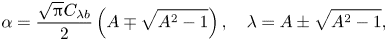 \begin{equation} \alpha=\frac{\sqrt{\rm \pi}C_{\lambda b}}{2}\left(A\mp\sqrt{A^2-1}\right), \quad \lambda =A\pm\sqrt{A^2-1}, \end{equation}
where  $A={\rm \pi} C_g^3C_{\lambda b}^2/\sqrt {2}, k_1=2A/\sqrt {A^2-1}\mp 1, {k_2=3A/\sqrt {A^2-1}}, {k_3=2A/\sqrt {A^2-1}}$ and ${k_4=3A/\sqrt {A^2-1}}$. Algebraically, this coefficient pair has two solutions, the implications of which are discussed in § 4.4, where we conclude that $\lambda >1$. Accordingly, the appropriate solutions are given by the upper part in the plus–minus symbols in the above equations.
(vii) The relationships for the pair  ${(C_{\lambda b},C_{Q})}$ are
 \begin{equation}
\alpha=C_Q^{3/2}\sqrt{\frac{\sqrt{2A^2+1}-1}{8A}}, \quad
\lambda
=\sqrt{\frac{2}{\sqrt{2A^2+1}-1}},
\end{equation}
\begin{equation}
\alpha=C_Q^{3/2}\sqrt{\frac{\sqrt{2A^2+1}-1}{8A}}, \quad
\lambda
=\sqrt{\frac{2}{\sqrt{2A^2+1}-1}},
\end{equation}
where  $A=C_Q^3/({\rm \pi} C_{\lambda b}^2)$, $k_1=1/\sqrt {2A^2+1}$, $k_2=3A^2/(2A^2+1\,{-}\,\sqrt {2A^2+1}), k_3=2A^2/(2A^2+1-\sqrt {2A^2+1})$ and $k_4=3A^2/(2A^2+1-\sqrt {2A^2+1})$.
(viii) The relationships for the pair  ${(C_{w},C_{g})}$ are
 \begin{equation} \alpha=\frac{\sqrt{2C_g^2+C_w^4}}{2C_w^3C_g}, \quad \lambda =\frac{C_w^2}{\sqrt{2}C_g}. \end{equation}
For this pair,  $k_1=(6C_g^2+C_w^4)/(2C_g^2+C_w^4), k_2=C_w^4/(2C_g^2+C_w^4), k_3=2$ and $k_4=1$.
(ix) The relationships for the pair  ${(C_{w},C_{Q})}$ are
 \begin{equation} \alpha=\frac{C_Q}{2C_w}, \quad \lambda =\sqrt{A-1}, \end{equation}
where  $A=C_w^4C_Q^2/2, k_1=1, k_2=1, k_3=2A/(A-1)$ and $k_4=A/(A-1)$.
(x) The relationships for the pair  ${(C_{g},C_{Q})}$ are
 \begin{equation} \alpha=\frac{C_Q^{3/2}}{2^{5/4}}\left({\frac{A}{A+1}}\right)^{1/4}, \quad \lambda =\frac{1}{\sqrt{A}}, \end{equation}
where  $A=C_Q^2C_g^2-1$, $k_1=1/(2A)$, $k_2=(3A+1)/(2A)$, $k_3=(A+1)/A$ and $k_4=(A+1)/A$.
(xi) The relationships for the pair  ${(C_{Q},C_{M})}$ are
 \begin{equation} \alpha=\frac{C_Q^2}{2^{3/2}C_M}, \quad \lambda =\sqrt{A-1}, \end{equation}
where  $A=2C_M^4/C_Q^2, k_1=2, k_2=1, k_3=A/(A-1)$ and $k_4=2A/(A-1)$.
(xii) The relationships for the pair  ${(C_{g},C_{B})}$ are
 \begin{equation} \alpha=\sqrt{\frac{C_g^6}{2C_B^6}+\frac{1}{4C_B^2}}, \quad \lambda =\frac{C_B^2}{\sqrt{2}C_g^3}. \end{equation}
For this pair,  $k_1=6C_g^6/(2C_g^6+C_B^4), k_2=(6C_g^6+C_B^4)/(2C_g^6+C_B^4), k_3=3$ and $k_4=2$.
Appendix B. Non-Boussinesq effects
Yuan & Cox (Reference Yuan and Cox1996) measured temperature differences of  $1000$ K (approximately) near the plume source and we estimate $\rho /\rho _e\approx 300/(1000+300)\approx 0.23$, i.e. a density ratio indicative of non-Boussinesq behaviour. However, as the plume rises and entrains cooler ambient air $\rho /\rho _e \rightarrow 1$, and the plume will approach its Boussinesq equilibrium state. Their measurements of centreline velocity and temperature show that the scalings expected for a Boussinesq pure plume begin at the visible flame height (approximately). This is despite the temperature difference here (of circa $200$ K) corresponding to a density ratio of $\rho /\rho _e\approx 300/(200+300)\approx 0.6$.
Rouse et al. (Reference Rouse, Yih and Humphreys1952) and Lee & Emmons (Reference Lee and Emmons1961) do not provide raw temperature measurements or flame heights that can be directly compared with those of Yuan & Cox (Reference Yuan and Cox1996). However, the Rouse et al. (Reference Rouse, Yih and Humphreys1952) description of a ‘low’ flame suggests that their measurements were above the visible flame height, and Lee & Emmons (Reference Lee and Emmons1961) report source width and fuel consumption rates that correspond to heat inputs per unit length similar to those of Yuan & Cox (Reference Yuan and Cox1996). The largest temperature difference that Yokoi (Reference Yokoi1960) reports for his centreline measurements is only  $44$ K. Comparisons of these observations with the data of Yuan & Cox (Reference Yuan and Cox1996) lends support to the view that non-Boussinesq effects did not unduly impact any of these three sets of measurements.
Additional support for this statement is provided by the non-Boussinesq plume model of van den Bremer & Hunt (Reference van den Bremer and Hunt2014b), which can be applied to assess the impact of the source density ratio on the evolution of the plume velocity and buoyancy. Their model shows that non-Boussinesq effects reduce the distance for a plume to approach the pure-plume equilibrium state relative to a Boussinesq plume with otherwise identical source conditions. As such, there is no clear justification to subject the far-field data gathered from plumes above fires to additional scrutiny. As is the case for Boussinesq plumes, the only requirement is that this equilibrium state has been (approximately) reached, which is the case for all of the experiments listed in table 3.
Appendix C. Analysis of the Kotsovinos (Reference Kotsovinos1975) data
The interpretation of the coefficient values based on the Kotsovinos (Reference Kotsovinos1975) dataset is not straightforward as there are inconsistencies between values reported in the thesis (Kotsovinos Reference Kotsovinos1975) and the related paper (Kotsovinos & List Reference Kotsovinos and List1977). For the profile widths, there are two choices:  $C_b=0.097/\sqrt {\ln {2}}=0.117$ and $C_{\lambda b}=0.13/\sqrt {\ln {2}}=0.156$ (paper, figure 7) or $C_b=0.10 /\sqrt {\ln {2}}=0.120$ and $C_{\lambda b}=0.14/\sqrt {\ln {2}}=0.168$ (thesis, Conclusions). Furthermore, these values are, in part, based on measurements of forced plumes ( $0<\varGamma <1$) which had not transitioned to the pure-plume-like region ( $\varGamma \approx 1$). While Kotsovinos (Reference Kotsovinos1975) and Kotsovinos & List (Reference Kotsovinos and List1977) both argue that the spreading rate of jets, forced plumes and pure plumes are equivalent, it is not clear that their measurements fully support their claim. Indeed, their measurements suggest that the buoyancy profile is consistently narrower for plume-like flows than jet-like flows (figure 7, Kotsovinos & List Reference Kotsovinos and List1977).
To ensure consistency with the other reported measurements (table 3), and to sidestep the question of which reported values to use, we reanalysed the Kotsovinos (Reference Kotsovinos1975) dataset in order to determine  $C_b$ and $C_{\lambda b}$ only from measurements in the pure-plume-like region. Using the same approach as in § 5, we calculated $\varGamma _0$ for each experiment and used the van den Bremer & Hunt (Reference van den Bremer and Hunt2014a) solutions to calculate $z_p$. For each experiment with at least two measurements where $z_m>z_p, C_b$ and $C_{\lambda b}$ were determined from a least-squares linear fit to the width-against-distance data. The average values are: $C_b=0.111$, from six experiments with a standard deviation of $10\,\%$, and $C_{\lambda b}=0.142$, from eight experiments with a standard deviation of $5\,\%$.
The new value  $C_b=0.111$ is very similar to the two previously reported values (Kotsovinos Reference Kotsovinos1975; Kotsovinos & List Reference Kotsovinos and List1977), but we note that this lower value of $C_b$ results in $\alpha =0.10$ (to 2 s.f.) rather than $\alpha =0.11$ as reported by Kotsovinos (Reference Kotsovinos1975) (Kotsovinos & List (Reference Kotsovinos and List1977) do not report an experimentally determined value for $\alpha$). Our proposed value of $C_{\lambda b}$ is significantly lower than both reported values, and, as a result, we conclude that the Kotsovinos (Reference Kotsovinos1975) dataset shows $\lambda =1.28$, rather than $\lambda =1.35$ as reported by Kotsovinos & List (Reference Kotsovinos and List1977) or $\lambda =1.4$ as implied by the values in Kotsovinos (Reference Kotsovinos1975).
As Kotsovinos (Reference Kotsovinos1975) and Kotsovinos & List (Reference Kotsovinos and List1977) both reported  $C_w=1.66$ and ${\sigma _T=1/C_g=0.42}$, as determined from measurements in the pure-plume-like region, we did not reanalyse their centreline data.
Appendix D. Analysis of the Parker et al. (Reference Parker, Burridge, Partridge and Linden2020) data
Parker et al. (Reference Parker, Burridge, Partridge and Linden2020) provide velocity and buoyancy data in the  $x-z$ plane for five experiments, which we used to calculate coefficients and create the plots herein. Parker et al. (Reference Parker, Burridge, Partridge and Linden2020) only reported values for $\alpha _T$ and $C_Q$ when scaled with $B_{0,S}$.
Figure 10 shows that the buoyancy flux measured in each of these experiments is approximately conserved, that the turbulent buoyancy flux is a small proportion of the mean, and that there is generally a significant discrepancy between the source buoyancy flux and the measured buoyancy flux. Averaged across the five experiments, the turbulent buoyancy flux is approximately  $10\,\%$ of the mean. For each experiment, $B_{0,M}$ and $B_{0,T}$ were determined as the average of the mean and total buoyancy fluxes over the height of the measured region.
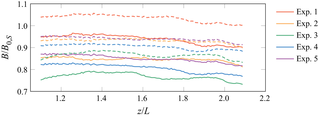
Figure 10. Variation of the plume buoyancy flux normalised by the source buoyancy flux with distance from the source. The solid lines show the mean buoyancy flux and dashed lines show the sum of the mean buoyancy flux and the turbulent vertical buoyancy flux. Plot based on data taken from Parker et al. (Reference Parker, Burridge, Partridge and Linden2020).
Figure 11 shows the profiles of mean vertical velocity and buoyancy scaled using  $B_{0,S}, B_{0,M}$ or $B_{0,T}$ and the distance from the virtual origin $z_0$. Following Parker et al. (Reference Parker, Burridge, Partridge and Linden2020), $z_0$ is calculated by extrapolating the top-hat plume width ( $2b_T=Q^2/M$) to zero. There are marginally improved collapses with $B_{0,M}$ or $B_{0,T}$, although the differences are small away from the centreline.
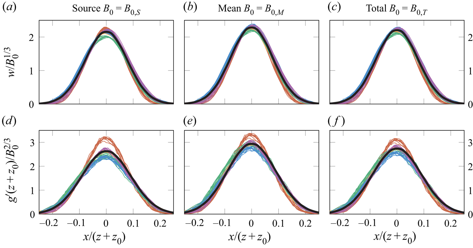
Figure 11. Scaled profiles of (a–c) plume vertical velocity and (d–f) buoyancy using data from Parker et al. (Reference Parker, Burridge, Partridge and Linden2020). The profiles are scaled by (a,d)  $B_{0,S}$, (b,e) $B_{0,M}$ and (c,f) $B_{0,T}$. The black lines show Gaussian fits to the data, with the coefficients listed in table 7.
Table 7. Average of the coefficients determined from the experimental data recorded by Parker et al. (Reference Parker, Burridge, Partridge and Linden2020) in their five experiments. The percentage uncertainty is the  $95\,\%$ confidence interval.
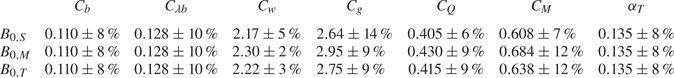
The values of the coefficients were determined for each of the five experiments from least-squares fits to the data, and the averages, together with the  $95\,\%$ confidence intervals, are shown in table 7. The choice of scaling (by $B_{0,S}, B_{0,M}$ or $B_{0,T}$) affects the values of some of the coefficients, and consequently the calculated values of $\alpha$ (§ 4.7).
Appendix E. Analysis of the Ramaprian & Chandrasekhara (Reference Ramaprian and Chandrasekhara1989) data
Ramaprian & Chandrasekhara (Reference Ramaprian and Chandrasekhara1989) normalised their coefficients using the total buoyancy flux. For comparison purposes, we calculated the coefficients if the mean buoyancy flux is used instead. We estimate (below) that their measurements show  $B_{0,M}/B_{0,T}=0.88$, and thus calculate the set: $C_w=2.22, C_g=2.79, C_Q=0.501$ and $C_M=0.806$ (all to 3 s.f.).
Ramaprian & Chandrasekhara (Reference Ramaprian and Chandrasekhara1989) reported that the magnitude of the kinematic turbulent heat-flux integral is  $0.18$. While not explicitly stated, their text and plot (figure 7(c) in their paper, where we have assumed that the $y$-axis label has a typographical error and $\overline {ut}/U_m^2$ should read $\overline {ut}/U_m{\rm \Delta} T_m$ in their notation) suggests that this value was normalised by the product of the centreline vertical velocity, centreline temperature and the width of the temperature profile. After accounting for the difference in convention regarding the plume width (by multiplying $0.18$ by $\sqrt {\ln {2}}$), their measurements of the turbulent component of the buoyancy flux $B_T$ show
 \begin{equation} \frac{B_T}{w_cg'_c\lambda b}=0.15. \end{equation}
Assuming Gaussian profiles of velocity and buoyancy, the mean buoyancy flux  $B_{0,M}$ is
 \begin{equation} B_{0,M}=\sqrt{\frac{\rm \pi}{\lambda^2+1}}w_cg'_c\lambda b=1.13w_cg'_c\lambda b, \end{equation}
where  $\lambda =1.21$, as calculated using the Ramaprian & Chandrasekhara (Reference Ramaprian and Chandrasekhara1989) measurements for $(C_{b},C_{\lambda b})$, was used to evaluate the prefactor. Combining (E1) and (E2), their turbulent flux measurements show that $B_T= 0.13 B_{0,M}$. This measurement can additionally be used to relate $B_T$ and $B_{0,M}$ to the total buoyancy flux: $B_T=0.12 B_{0,T}$ and $B_{0,M}=0.88 B_{0,T}$.


 Open access