


1. Introduction
Recent successes in the application of artificial intelligence (AI) methods to fluid dynamics cover a wide range of topics. These include model building such as a data-driven identification of suitable Reynolds-averaged Navier–Stokes models (Duraisamy, Iaccarino & Xiao Reference Duraisamy, Iaccarino and Xiao2019; Rosofsky & Huerta Reference Rosofsky and Huerta2020), subgrid-scale parametrisations (Rosofsky & Huerta Reference Rosofsky and Huerta2020; Xie et al. Reference Xie, Wang, Li, Wan and Chen2020), state estimation by neural networks based on reduced-order models (Nair & Goza Reference Nair and Goza2020), data assimilation for rotating turbulence (Buzzicotti et al. Reference Buzzicotti, Bonaccorso, Leoni and Biferale2021) through generative adversarial networks (Goodfellow et al. Reference Goodfellow, Pouget-Abadie, Mirza, Xu, Warde-Farley, Ozair, Courville and Bengio2014), dynamical and statistical prediction tasks (Srinivasan et al. Reference Srinivasan, Guastoni, Azizpour, Schlatter and Vinuesa2019; Boullé et al. Reference Boullé, Dallas, Nakatsukasa and Samaddar2020; Lellep et al. Reference Lellep, Prexl, Linkmann and Eckhardt2020; Pandey & Schumacher Reference Pandey and Schumacher2020; Pandey, Schumacher & Sreenivasan Reference Pandey, Schumacher and Sreenivasan2020) or pattern extraction in thermal convection (Schneide et al. Reference Schneide, Pandey, Padberg-Gehle and Schumacher2018; Fonda et al. Reference Fonda, Pandey, Schumacher and Sreenivasan2019). Open questions remain as to how AI can be used to increase our knowledge of the physics of a turbulent flow, which in turn requires knowledge as to what data features a given machine learning (ML) method bases its decisions upon. This is related to the question of representativeness vs significance introduced and discussed by Jiménez (Reference Jiménez2018) in the context of two-dimensional homogeneous turbulence and motivates the application of explainable AI.
Lately, advances in model agnostic explanation techniques have been made by Lundberg & Lee (Reference Lundberg and Lee2017) in the form of the introduction of Shapley additive explanations (SHAP) values. These techniques have proven themselves useful in a wide range of applications, such as decreasing the risk of hypoxaemia during surgery (Lundberg et al. Reference Lundberg2018b) by indicating the risk factors on a per-case basis. Subsequently, these methods have been adapted and optimised for tree ensemble methods (Lundberg, Erion & Lee Reference Lundberg, Erion and Lee2018a). Here, we use boosted trees as well as deep neural networks in conjunction with SHAP values to provide a first conceptual step towards a machine-assisted understanding of relaminarisation events in wall-bounded shear flows.
Relaminarisation describes the collapse of turbulent transients onto a linearly stable laminar flow profile. It is intrinsically connected with the transition to sustained turbulence in wall-bounded shear flows. Localised turbulent patches such as puffs in pipe flow either relaminarise or split in two (Wygnanski & Champagne Reference Wygnanski and Champagne1973; Nishi et al. Reference Nishi, Ünsal, Durst and Biswas2008; Avila et al. Reference Avila, Moxey, de Lozar, Avila, Barkley and Hof2011). Transient turbulence is explained in dynamical systems terms through a boundary crisis between a turbulent attractor and a lower branch of certain exact solutions of the Navier–Stokes equations (Kawahara & Kida Reference Kawahara and Kida2001; Kreilos & Eckhardt Reference Kreilos and Eckhardt2012; Lustro et al. Reference Lustro, Kawahara, van Veen, Shimizu and Kokubu2019). In consequence, the boundary of the basin of attraction of the laminar fixed point becomes fractal, and the turbulent attractor transforms into a chaotic saddle. Relaminarisation events correspond to state-space trajectories originating within this complex basin of attraction of the laminar state, eventually leaving the chaotic saddle in favour of the laminar fixed point. For an ensemble of state-space trajectories, the hallmark of escape from a chaotic saddle – a memoryless process – is an exponential sojourn time distribution  $P(t) \propto \exp {(t/\tau )}$, with $P(t)$ denoting the probability of residing within the strange saddle after time $t$ and $\tau$ the characteristic time scale of the escape (Ott Reference Ott2002). Exponentially distributed sojourn times, or turbulent lifetimes, are a salient feature of wall-bounded turbulence close to onset, for instance in pipe flow (Hof et al. Reference Hof, Westerweel, Schneider and Eckhardt2006; Eckhardt et al. Reference Eckhardt, Schneider, Hof and Westerweel2007; Hof et al. Reference Hof, de Lozar, Kuik and Westerweel2008; Avila, Willis & Hof Reference Avila, Willis and Hof2010; Avila et al. Reference Avila, Moxey, de Lozar, Avila, Barkley and Hof2011) or plane Couette flow (Schmiegel & Eckhardt Reference Schmiegel and Eckhardt1997; Bottin et al. Reference Bottin, Daviaud, Manneville and Dauchot1998; Eckhardt et al. Reference Eckhardt, Schneider, Hof and Westerweel2007; Schneider et al. Reference Schneider, Lillo, Buehrle, Eckhardt, Dörnemann, Dörnemann and Freisleben2010; Shi, Avila & Hof Reference Shi, Avila and Hof2013), and they occur in box turbulence with periodic boundary conditions provided the forcing allows relaminarisation (Linkmann & Morozov Reference Linkmann and Morozov2015). The associated time scale $\tau$ usually increases super-exponentially with Reynolds number (Eckhardt & Schneider Reference Eckhardt and Schneider2008; Hof et al. Reference Hof, de Lozar, Kuik and Westerweel2008; Avila et al. Reference Avila, Moxey, de Lozar, Avila, Barkley and Hof2011; Linkmann & Morozov Reference Linkmann and Morozov2015). The puff splitting process also has a characteristic Reynolds-number-dependent time scale, and the transition to sustained and eventually space-filling turbulence occurs when the puff splitting time scale exceeds the relaminarisation time scale (Avila et al. Reference Avila, Moxey, de Lozar, Avila, Barkley and Hof2011). In the language of critical phenomena, the subcritical transition to turbulence belongs to the directed percolation universality class (Pomeau Reference Pomeau1986; Lemoult et al. Reference Lemoult, Shi, Avila, Jalikop and Hof2016).
In order to facilitate the physical interpretation and to save computational effort, in this first step we consider a nine-dimensional shear flow model (Moehlis, Faisst & Eckhardt Reference Moehlis, Faisst and Eckhardt2004) that reproduces the aforementioned turbulence lifetime distribution (Moehlis et al. Reference Moehlis, Faisst and Eckhardt2004) of a wall-bounded parallel shear flow. Subsequently, and in order to demonstrate that the method can be upscaled to larger datasets relevant to fluid dynamics applications, we provide an example, where the same classification task is carried out on data obtained by direct numerical simulation (DNS) of plane Couette flow in a minimal flow unit. Here, we focus on the structure of high- and low-speed streaks characteristic of near-wall turbulence.
The low-dimensional model is obtained from the Navier–Stokes equations by Galerkin truncation and the basis functions are chosen to incorporate the self-sustaining process (SSP) (Waleffe Reference Waleffe1997), which describes the basic nonlinear near-wall dynamics of wall-bounded parallel shear flows close to the onset of turbulence. According to the SSP, a streak is generated by advection of the laminar flow by a streamwise vortex, this streak is linearly unstable to spanwise and wall-normal perturbations, which couple to re-generate the streamwise vortex and the process starts anew. The nine-dimensional model assigns suitably constructed basis functions to the laminar profile, the streamwise vortex, the streak and its instabilities and includes a few more degrees of freedom to allow for mode couplings. Each basis function, that is, each feature for the subsequent ML steps, has a clear physical interpretation. Hence, the model lends itself well for a first application of explainable AI methods to determine which flow features are significant for the prediction of relaminarisation events.
The nine-mode model by Moehlis et al. (Reference Moehlis, Faisst and Eckhardt2004) and similar low-dimensional models have been considered in a number of contributions addressing fundamental questions in the dynamics of parallel shear flows. Variants of the nine-mode model have been used, for instance, to introduce the concept of the edge of chaos to fluid dynamics and its connection with relaminarisation events (Skufca, Yorke & Eckhardt Reference Skufca, Yorke and Eckhardt2006), to understand drag reduction in viscoelastic fluids (Roy et al. Reference Roy, Morozov, van Saarloos and Larson2006) or to develop data-driven approaches to identify extreme fluctuations in turbulent flows (Schmid, García-Gutierrez & Jiménez Reference Schmid, García-Gutierrez and Jiménez2018). In the context of AI, Srinivasan et al. (Reference Srinivasan, Guastoni, Azizpour, Schlatter and Vinuesa2019) used different types of neural networks (NNs) to predict the turbulent dynamics of the nine-dimensional model. There, the focus was on the ability of NNs to reproduce the shear flow dynamics and statistics with a view towards the development of machine-assisted subgrid-scale models. Good predictions of the mean streamwise velocity and Reynolds stresses were also obtained with echo state networks (ESNs) (Pandey et al. Reference Pandey, Schumacher and Sreenivasan2020). Doan, Polifke & Magri (Reference Doan, Polifke and Magri2019) used physics-informed ESNs, where the equations of motion are incorporated as an additional term in the loss function, for dynamical prediction of chaotic bursts related to relaminarisation attempts.
The key contribution in our work is to identify the significant features within a data-driven prediction of relaminarisation events, that is, the features a classifier needs to see in order to perform well. For the nine-mode model (NMM), apart from the laminar profile, we find that SHAP identifies some of the main constituents of the SSP, the streamwise vortex and a single sinusoidal streak instability, as important for the prediction of relaminarisation events. Other features, such as the streak mode or certain streak instabilities, which are certainly of relevance for the dynamics, are not identified. These strongly correlate with the features that have been identified as important for the classification, hence they carry little additional information for the classifier. There is no a priori reason for choosing, say, the streamwise vortex instead of the streak as a feature relevant for the prediction. In fact, if predictions are run using only subsets consisting of features that have not been identified as important but correlate with important features, the prediction accuracy drops significantly. Finally, the information provided by SHAP is discussed in conjunction with the model equations to provide physical insights into the inner workings of the SSP within the remit of the NMM. For the DNS data, SHAP values indicate that the classifier bases its decisions on regions in the flow that can be associated with streak instabilities. This suggests SHAP as a method to inform the practitioner as to which flow features carry information relevant to the prediction of relaminarisation events, information that cannot be extracted by established means.
The remainder of this article is organised as follows. We begin with an introduction of the NMM, its mathematical structure and dynamical phenomenology in § 2. Subsequently, § 3 summarises the technical details of the ML approach, that is, boosted trees for the classification and SHAP values for the interpretation. The results of the main investigation are presented in § 4. First, we summarise the prediction of relaminarisation events. Second, the most important features, here the physically interpretable basis functions of the aforementioned NMM, are identified by ranking according to the mean absolute SHAP values for a number of prediction time horizons. Short prediction times, where the nonlinear dynamics is already substantially weakened, serve as validation cases. As expected, the laminar mode is the only relevant feature in the prediction in such cases. For longer prediction times the laminar mode remains important, and the modes corresponding to the streamwise vortex and the sinusoidal streak instability become relevant. Therein, § 4.3 contains a critical discussion and interpretation of the results described in the previous sections. Here, we connect the significant features identified by SHAP to important human-observed characteristics of wall-bounded shear flows such as streaks and streamwise vortices in the SSP. Section 5 provides an example SHAP calculation on DNS data of plane Couette flow in a minimal flow unit. We summarise our results and provide suggestions for further research in § 6 with a view towards the application and extension of the methods presented here to higher-dimensional data obtained from experiments or high-resolution numerical simulations.
2. The NMM
We begin with a brief description of the NMM (Moehlis et al. Reference Moehlis, Faisst and Eckhardt2004) and its main features. The model is obtained by Galerkin truncation of a variation of plane Couette flow with free-slip boundary conditions at the confining walls, the sinusoidal shear flow. Sinusoidal shear flows show qualitatively similar behaviour compared with canonical shear flows such as pipe and plane Couette flow, in the sense that (i) the dynamics is governed by the SSP (Waleffe Reference Waleffe1997), and (ii) the laminar profile is linearly stable for all Reynolds numbers (Drazin & Reid Reference Drazin and Reid2004). Most importantly, the sinusoidal shear flow we use subcritically transitions to turbulence and shows relaminarisation events, it is thus a prototypical example of a wall-bounded shear flow.
More precisely, we consider an incompressible flow of a Newtonian fluid between two – in principle – infinitely extended parallel plates a distance  $d$ apart, with free-slip boundary conditions in the wall-normal $x_2$-direction. Periodic boundary conditions in the homogeneous streamwise ( $x_1$) and spanwise ( $x_3$) directions model the infinite extent of the plates. The sinusoidal shear flow is thus described by the incompressible Navier–Stokes equations in a rectangular domain $\varOmega = [0,L_1] \times [-d/2,d/2] \times [0,L_3]$. These read in non-dimensionalised form
 $$\begin{gather} \frac{\partial \boldsymbol{u}}{\partial t} + (\boldsymbol{u}\boldsymbol{\cdot}\boldsymbol{\nabla})\boldsymbol{u} ={-}\boldsymbol{\nabla} p + \frac{1}{{Re}} \boldsymbol{\Delta} \boldsymbol{u} + \frac{\sqrt{2}{\rm \pi}^{2}}{4{Re}}\sin({\rm \pi} x_2 / 2)\boldsymbol{\hat{e}}_{x_1}, \end{gather}$$
 $$\begin{gather}\boldsymbol{\nabla}\boldsymbol{\cdot}\boldsymbol{u} = 0, \end{gather}$$
where  $\boldsymbol {u}(\boldsymbol {x}=(x_1, x_2, x_3))=(u_1, u_2, u_3)$ is the fluid velocity, $p$ is the pressure divided by the density and ${Re}=U_0 d/(2 \nu )$ the Reynolds number based on the kinematic viscosity $\nu$, the velocity of the laminar flow $U_0$ and the distance $d$ between the confining plates, and $\hat {\boldsymbol {e}}_{x_1}$ the unit vector in the streamwise direction. The last term on the right-hand side of (2.1) corresponds to an external volume force, which is required to maintain the flow owing to the free-slip boundary conditions. It sustains the laminar profile $\boldsymbol {U}(x_2) = \sqrt {2}\sin ({\rm \pi} x_2 / 2)\hat {\boldsymbol {e}}_{x_1}$ and determines thereby the velocity scale $U_0$, which is given by $\boldsymbol {U}(x_2)$ evaluated at a distance $x_2 = d/4$ from the top plate. The non-dimensionalisation with respect to $U_0$ and $d/2$ results in time being given in units of $d/(2U_0)$.
The NMM of Moehlis et al. (Reference Moehlis, Faisst and Eckhardt2004) is a low-dimensional representation of the sinusoidal shear flow obtained by Galerkin projection onto a subspace spanned by nine specifically chosen orthonormal basis functions  $\boldsymbol {u}_i(\boldsymbol {x})$ for $i = 1, \ldots, 9$ with $\langle \boldsymbol {u}_i(\boldsymbol {x}), \boldsymbol {u}_j(\boldsymbol {x}) \rangle = \delta _{ij}$, where $\langle \cdot \rangle$ denotes the $L_2$-inner product on $\varOmega$. The NMM extends previous models by Waleffe with 4 and 8 modes (Waleffe Reference Waleffe1995, Reference Waleffe1997) based on the SSP. Each mode has a clear interpretation

The basis functions, or modes, are divergence free and satisfy the aforementioned boundary conditions. We refer to (7) to (16) of Moehlis et al. (Reference Moehlis, Faisst and Eckhardt2004) for the explicit mathematical expressions. The Galerkin projection results in the following expansion:
 \begin{equation} \boldsymbol{u}(\boldsymbol{x}, t) = \sum_{i=1}^{9} a_i(t) \boldsymbol{u}_i(\boldsymbol{x}), \end{equation}
for the velocity field with nine corresponding time-dependent coefficients  $a_i(t)$. Equation (2.1) then gives rise to a system of nine ordinary differential equations for $a_1(t), \ldots, a_9(t)$ – the NMM – given by (21) to (29) of Moehlis et al. (Reference Moehlis, Faisst and Eckhardt2004). Despite its simplicity, the dynamics of the NMM resembles that of wall-bounded shear flows close to the onset of turbulence which transition subcritically. First, it is based on the near-wall cycle, the SSP, by construction. Secondly, its transient chaotic dynamics collapses onto the laminar fixed point with exponentially distributed lifetimes (Moehlis et al. Reference Moehlis, Faisst and Eckhardt2004, figure 7), that is, it shows relaminarisation events with qualitatively similar statistics as wall-bounded parallel shear flows. Hence, the model is suitable for a study concerned with the prediction of relaminarisation events of turbulent shear flows.
The nine ordinary differential equations that comprise the NMM are solved with an explicit Runge–Kutta method of order 5 (Dormand & Prince Reference Dormand and Prince1980) with a fixed time step, using Scipy (Virtanen et al. Reference Virtanen2020) with Python. The time step for the integrator is set to  $dt=0.25$ for all simulations and we use a simulation domain of size $[0,4{\rm \pi} ] \times [-1,1] \times [0,2{\rm \pi} ]$ in units of $d/2$. Since we later train ML models to predict the relaminarisation events, a Reynolds number of ${Re}=250$ is chosen in order to reduce waiting times for relaminarisation events, as the mean turbulent lifetime increases very rapidly with Reynolds number. Figure 1 presents a time series of $a_1(t), \ldots, a_9(t)$ representative of a relaminarisation event in the NMM. After irregular fluctuations, eventually the coefficients $a_2(t), \ldots, a_9(t)$, pertaining to all but the laminar mode, decay. In contrast, the coefficient $a_1(t)$ of the laminar mode, shown in red, asymptotes to unity. The chaotic regions of the dynamics of the NMM are characterised by a Lyapunov time of $t_{L} \approx 60$. The Lyapunov time is the inverse of the largest Lyapunov exponent (Ott Reference Ott2002) and corresponds to the time after which initially infinitesimally close phase-space trajectories become separated by an $L_2$-distance of $e$, Euler's number.

Figure 1. Time series of the nine spectral coefficients  $a_i$ in (2.3), with the laminar coefficient $a_1$ shown in black and modes $a_2$ to $a_9$ are shown in red to yellow. The dashed green line represents the threshold between turbulent and laminar dynamics as defined by an energy threshold on the deviations of the laminar profile $E_l = 5 \times 10^{-3}$, see (4.1). The number of snapshots per training sample is set to $N_s=5$, which are $\Delta t$ apart. The temporal spacing is set to $\Delta t=100$ in this example for visual purposes only, $\Delta t=3$ is used in all calculations with $N_s > 1$. The short orange vertical lines mark prediction time horizons of $t_p=\{200,300,350\}$ for visual guidance, see § 4 for further details.
3. ML and SHAP values
3.1. XGBoost
A gradient boosted tree model is used as ML model for making the relaminarisation predictions. Specifically, the XGBoost (Chen & Guestrin Reference Chen and Guestrin2016) implementation of a boosted tree model in Python is utilised to benefit from its fast implementation for very large datasets. XGBoost is known for its high performances on ML tasks such as high energy physics event classification, massive online course dropout rate predictions and other dedicated real-life ML competition tasks (Chen & Guestrin Reference Chen and Guestrin2016). Additionally, XGBoost-based classifiers benefit from fast implementations of SHAP value computations (Lundberg et al. Reference Lundberg, Erion and Lee2018a) that will be used in § 4.2 to explain the trained ML model.
Boosting methods belong to the class of ensemble methods (Hastie, Tibshirani & Friedman Reference Hastie, Tibshirani and Friedman2009). These methods use an ensemble of weak learners, i.e. models that by themselves are not very powerful, to make predictions. The mathematical details of boosted trees and XGBoost can be found in Appendix A.1.
3.2. SHAP values
While ML models might show good prediction performances given a task, it is not per se clear which relations have been learned and led to this good performance. Complex and well-performing ML models come at the cost of being difficult to be interpreted and inspected. Hence, traditionally less performing methods, such as linear models, were deployed for the sake of being easier to interpret. Recent advances in explainable AI attempt to work on the understanding of well-performing and complex ML models – including model agnostic explanation techniques and model-specific explanation techniques – to benefit from high prediction performances as well as explainable models.
One recent method that enables complex models to be interpreted are SHAP values. SHAP values unify recently developed explainable AI methods such as the LIME (Ribeiro, Singh & Guestrin Reference Ribeiro, Singh and Guestrin2016), DeepLIFT (Shrikumar, Greenside & Kundaje Reference Shrikumar, Greenside and Kundaje2017) and layer-wise relevance propagation (Bach et al. Reference Bach, Binder, Montavon, Klauschen, Müller and Samek2015) algorithms while also demonstrating theoretically that SHAP values provide multiple desirable properties. Additionally, SHAP values can be evaluated efficiently when using model-specific implementations such as for XGBoost. We briefly introduce SHAP values in the following.
SHAP values belong to the class of additive feature explanation models that explain the ML model output  $g$ at sample $\boldsymbol {z}\in \mathbb {R}^{M}$ in terms of effects assigned to each of the features
 \begin{equation} g(\boldsymbol{z}) = \varPhi_0 + \sum_{m=1}^{M} \varPhi_m, \end{equation}
with  $M$ as number of features. Lundberg & Lee (Reference Lundberg and Lee2017) define a specific choice of $\varPhi _m$ which they coined as SHAP values. These are based on the game-theoretic Shapley values (Shapley Reference Shapley1953) and adhere to three desirable properties that make their explanations locally accurate and consistent. The SHAP value for feature $m$ of sample $\boldsymbol {z}$ for model $g$ are computed as
 \begin{equation} \varPhi_m(g, \boldsymbol{z}) = \sum_{S \subseteq S_F \setminus \{m\}} \frac{|S|! (M - |S| - 1)!}{M!} (g(S\cup \{m\}) - g(S)) \end{equation}
with  $S$ a subset of features that does not contain the feature $m$ to be explained, $S_F$ the set of all $M$ features and $g(S)$ as model output of feature subset $S$;
$S$;  $\varPhi _0$ is determined separately as the average model output by $\varPhi _0=g(S=\emptyset )$.
Intuitively, SHAP values thereby measure the difference between the trained model evaluated including a particular target feature and evaluated excluding it, averaged over all feature set combinations that do not include the target feature. The prefactor is a symmetric weighting factor and puts emphasis on model output differences for feature subsets  $S$ with either a small number of features or a number close to $M$. Hence, the model output difference that stems from removing the target feature is considered particularly relevant when there is either a small or a large number of features in the feature set $S$ that is considered.
The model  $g$ evaluated on a feature subset $S$,
$S$,  $g(S)$, is technically challenging as a model is trained on a fixed number of features; $g(S)$ is realised by a conditional expectation value that conditions on the feature values of $\boldsymbol {z}$ that are present in feature subset $S$
$S$
 \begin{equation} g(S) = \mathbb{E}[g(\hat{\boldsymbol{z}}) \,|\, \hat{\boldsymbol{z}}=\boldsymbol{z}_S]. \end{equation}
This avoids the technical difficulty of evaluating a readily trained model on a subset of features.
The SHAP value property of local accuracy ensures that the sum of the SHAP values for the explained sample  $\boldsymbol {z}$ corresponds to the difference between the model output for that sample, $g(\boldsymbol {z})$, and the mean prediction of the model, $\langle g(\tilde {\boldsymbol {z}}) \rangle _{\tilde {\boldsymbol {z}}}$
 \begin{equation} \sum_{m=1}^{M} \varPhi_m(g, \boldsymbol{z}) = g(\boldsymbol{z}) - \langle g(\tilde{\boldsymbol{z}}) \rangle_{\tilde{\boldsymbol{z}}}. \end{equation}
Hence, the sum over all SHAP values is equal to the difference between model output and mean model prediction.
We use a fast implementation of SHAP values for tree ensemble models by Lundberg et al. (Reference Lundberg, Erion and Lee2018a). While (3.3) is typically evaluated by an integration over a background dataset, the fast tree-specific algorithm incorporates the tree structure by omitting all paths that are not compatible with the conditional values  $\boldsymbol {z}_S$.
While SHAP values provide per-sample contributions for each feature, a typical task is to assign each feature  $m=1,\ldots,M$ an importance for the model predictions. A common approach is to average the absolute SHAP values over all samples in the dataset (Molnar Reference Molnar2020). The average ensures a statistical statement about the SHAP values and removing the sign from the SHAP values ensures that positive and negative contributions to the ML model output are accounted for equally.
Additionally to the classical SHAP values presented above, there exist SHAP interaction values (Lundberg et al. Reference Lundberg, Erion, Chen, DeGrave, Prutkin, Nair, Katz, Himmelfarb, Bansal and Lee2020) that capture the contributions of feature interactions to the ML model output by generalising the classical SHAP values to combinations of features. Consequently, each sample is assigned a matrix of SHAP interaction values that are computed as
 \begin{align} \varPhi_{m,n}(g, \boldsymbol{z}) &= \sum_{S \subseteq S_F \setminus \{m,n\}} \frac{|S|! (M - |S| - 2)!}{2 (M-1)!} \left(g(S\cup \{m,n\}) - g(S\cup \{n\}) \right.\nonumber\\ &\quad \left. -[g(S\cup\{m\})-g(S)] \right), \end{align}
for  $m\neq n$ and
 \begin{equation} \varPhi_{m,m}(g, \boldsymbol{z}) = \varPhi_m(g,\boldsymbol{z}) - \sum_{n\neq m} \varPhi_{m,n}(g, \boldsymbol{z}). \end{equation}
Setting  $\varPhi _{0,0}(g, \boldsymbol {z})$ to the average output of $g$, one obtains a similar property as for the classical SHAP values in (3.4), namely the additivity property
 \begin{equation} \sum_{m=0}^{M} \sum_{n=0}^{M} \varPhi_{m,n}(g, \boldsymbol{z}) = g(\boldsymbol{z}). \end{equation}
Also for these SHAP interaction values we use a fast implementation for tree ensembles (Lundberg et al. Reference Lundberg, Erion, Chen, DeGrave, Prutkin, Nair, Katz, Himmelfarb, Bansal and Lee2020).
4. Results
Before studying the inner workings of the ML model, a well-performing model needs to be trained on relaminarisation events. This section defines the fluid dynamical classification task and presents the achieved results with a XGBoost tree followed by their explanation with SHAP values.
The prediction of the relaminarisation events a time  $t_p$ ahead is considered a supervised binary classification problem in ML (Bishop Reference Bishop2006). Supervised tasks require the training data to consist of pairs of input and target outputs, commonly called $\boldsymbol {z}$ and $y$, respectively. Here, the input data consist of a number $N_s$ of nine-dimensional vectors of spectral coefficients $\boldsymbol {a} = (a_1, \ldots, a_9)$ from the flow model introduced in § 2. The output is a binary variable encoded as $1$ and $0$ that contains information on whether the flow corresponding to the input spectral coefficients relaminarised a time $t_p$ ahead or not, respectively.
The training data are acquired by forward simulation of the flow model. A single fluid simulation is initialised with a random nine-dimensional initial condition, with initial amplitudes uniformly distributed according to  $U(-0.25,0.25)$, and integrated for $4000$ time units. After removing a transient period of $200$ time units to ensure that the dynamics has reached the attracting phase-space region, training samples for each of the two classes are extracted from the trajectory. This process of starting forward simulations of the fluid model and the subsequent extraction of training data is repeated until enough training samples have been obtained.
The training data comprise  $N_t=10^{6}$ training samples, half of which belong to the class of samples that relaminarise and the other half belong to the class of samples that do not relaminarise. The balanced test dataset is separate from the training dataset and consists of $N_v=10^{5}$ samples that have not been used for training purposes.
The extraction of training samples from a trajectory is based on the classification of the trajectory in turbulent and laminar regions. For that, the energy of the deviation from the laminar flow of each of the velocity fields  $\boldsymbol {u}(\boldsymbol {x}, t)$ in the trajectory is computed as
 \begin{equation} E(t) = \langle \boldsymbol{u}(\boldsymbol{x}, t) - \boldsymbol{U}(x_2), \boldsymbol{u}(\boldsymbol{x}, t) - \boldsymbol{U}(x_2) \rangle = \sum_{i=1}^{9} \left(a_i(t) - \delta_{1, i}\right)^{2}, \end{equation}
using the spectral expansion coefficients  $a_i(t)$ at each time step and the orthonormality of the basis functions in the last equality. To classify the trajectory in turbulent and laminar sections, an energy threshold $E_l = 5\times 10^{-3}$ is set. Hence, a velocity field $\boldsymbol {u}$ is classified according to the binary variable
 \begin{equation} c(\boldsymbol{u})
=\begin{cases} 1, & \text{if } E(\boldsymbol{u}) \le E_l \\
0, & \text{otherwise} \end{cases}
\end{equation}
\begin{equation} c(\boldsymbol{u})
=\begin{cases} 1, & \text{if } E(\boldsymbol{u}) \le E_l \\
0, & \text{otherwise} \end{cases}
\end{equation}
with  $c = 0$ denoting the class of samples that do not relaminarise $t_p$ time steps ahead and class $1$ denoting those that do relaminarise. The value for $E_l$ is chosen based on empirical tests that have shown no return to chaotic dynamics after a trajectory reached a velocity field with energy $E_l$.
Using the classification  $c(\boldsymbol {u}(t))$ of a trajectory $\boldsymbol {u}(t)$, the training data acquisition is characterised by the prediction horizon $t_p$ and the number of flow fields $N_s$ that make up one sample. To construct a single training sample from a trajectory, a random point $t_r$ in the trajectory is chosen to serve as target point. Its classification label $c(\boldsymbol {u}(t_r))$ is used as training data target output $y$. The input data $\boldsymbol {z}$ is obtained by using $N_s$ equally spaced spectral coefficients preceding the chosen time point about $t_p$, i.e. at $t_r - t_p$. Hence, a single training sample is extracted as
 \begin{equation} (\boldsymbol{z}, y) = \left(\left[\boldsymbol{a}(t_r - t_p - (N_s-1) \Delta t),\ldots, \boldsymbol{a}(t_r - t_p - 0 \Delta t)\right],\ c(\boldsymbol{u}(t_r))\right), \end{equation}
with the temporal spacing between subsequent snapshots for one training sample  $\Delta t$. We gauged $\Delta t=3$ to the dynamics of the flow model in order to capture sufficient dynamical detail. Finally, the temporal positions $t_r$ are spread randomly in turbulent regions to obtain samples for class $0$ and specifically placed at the laminar transition to obtain samples for class $1$.
$1$.
Figure 1 shows the training data acquisition process based on an example trajectory with one randomly chosen time  $t_{r,1}$ to obtain a sample for class $0$, coloured in blue, and another time $t_{r,2}$ set at the laminar transition to obtain a sample for class $1$, coloured in green. The short orange vertical lines mark the prediction time horizons of $t_p=\{200,300,350\}$ for visual guidance. The large value of $a_1$ for $t_p=200$ demonstrates why this prediction horizon serves as validation case. After training, the ML classifier can be given a set of $N_s$ points equally spaced with $\Delta t$ and predict whether the flow described by these data will relaminarise after a time integration of $t_p$ time units.
It is good practice to analyse the training data prior to training classifiers on it. We pick  $N_s=1$ and visualise the training data distributions of the nine spectral expansion coefficients for $t_p\in \{200, 300\}$, see figure 2. The distributions for the two classes $0$ and $1$ become statistically less distinguishable for increasing $t_p$, requiring the ML model to learn per-sample correlations to perform well. It is observed that the classes for $t_p=200$ can be distinguished from a statistical point of view already. This is because the prediction horizon is not large enough to move the samples off the slope of the laminar transition as indicated by the rightmost orange bar in figure 1. The prediction horizon of $t_p=300$, on the other hand, is large enough to forbid sample classification through simple statistical properties because the histograms of both classes mostly overlap. Hence, $t_p=200$ is considered a benchmark case as the prediction performance is expected to be high because the large laminar mode is sufficient for the classification.

Figure 2. Normalised training data distributions of modes  $1$ to $9$. Here, $t_p=300$ is shifted upwards for visual purposes. Class $1$ (
$1$ ( $0$) corresponds to samples that do (not) relaminarise after $t_p$ time steps.
4.1. Prediction of relaminarisation events
The hyperparameters of the gradient boosted tree are optimised using a randomised hyperparameter search strategy. The strategy chooses the hyperparameters from predefined continuous (discrete) uniform distributions  $U_c(a, b)$ ( $U_d(a, b$)) between values $a$ and $b$ and samples a fixed number of draws. We draw $100$ hyperparameter combinations according to the distributions
 \begin{equation} \left.\begin{gathered} h_{NE} \sim U_d(500, 1500), \\ h_{MD} \sim U_d(1, 50), \\ h_{MCW}\sim U_d(1, 15), \\ h_{GA} \sim U_c(0, 5), \\ h_{SS} \sim U_c(0.5, 1), \\ h_{CBT} \sim U_c(0.5, 1), \\ h_{LR} \sim U_c(0.001, 0.4). \end{gathered}\right\} \end{equation}
We verified for  $t_p=300$ that $100$ draws cover the hyperparameter phase space sufficiently well by drawing $200$ hyperparameter combinations to show that this leads to similar prediction performances as for $100$. The hyperparameters that are found by the randomised hyperparameter search are listed in Appendix A.2.
The prediction performance, measured on a test dataset, for  $N_s=1$ decays with increasing $t_p$, as expected on account of the intrinsic chaotic dynamics of the flow model (Moehlis et al. Reference Moehlis, Smith, Holmes and Faisst2002; Moehlis, Faisst & Eckhardt Reference Moehlis, Faisst and Eckhardt2005; Lellep et al. Reference Lellep, Prexl, Linkmann and Eckhardt2020), see figure 3. Nevertheless, the prediction performance is approximately $90\,\%$ for $5$ Lyapunov times (Bezruchko & Smirnov Reference Bezruchko and Smirnov2010) in the future and is, thereby, sufficiently good for the subsequent model explanations by SHAP values. Calculations for different values of $N_s$ verify that the prediction performance only varies marginally for one exemplary set of hyperparameters. This is to be expected based on the deterministic nature of the dynamical system and its full observability. Hence, we here focus on $N_s=1$, which means that the classifier does not get dynamical information but only a single spectral snapshot of the flow field. This reduces the computational cost for the subsequent model explanation by SHAP values.

Figure 3. Prediction performance of the trained classifier against temporal prediction horizon  $t_p$. The error bar for $t_p=300$ shows $100$ standard deviations $\sigma$ for visualisation purposes and demonstrates the robustness of the results. It has been obtained by training the classifier on training datasets based on different initial random number generator seeds.
The prediction horizon  $t_p=200$, indeed, corresponds to the benchmark case where the laminar mode is supposed to be the only relevant indicator for relaminarisation and $450$ corresponds to the case beyond which the ML model cannot predict reliably due to the chaotic nature of the system (Moehlis et al. Reference Moehlis, Smith, Holmes and Faisst2002, Reference Moehlis, Faisst and Eckhardt2005; Lellep et al. Reference Lellep, Prexl, Linkmann and Eckhardt2020).
Lastly, to demonstrate the performance of the ML model also for applied tasks, the model is applied in parallel to a running fluid simulation. Figure 4(a) shows the on-line prediction of one simulated trajectory. The horizontal bottom bar indicates whether the prediction of the classifier has been correct (green) or incorrect (red). We collected statistics over  $1000$ trajectories to quantify how well the model performs on an applied task instead of the test dataset. As shown in figure 4(b), the model performance for the on-line live prediction is with approximately $90\,\%$ true positives and true negatives as well as approximately $10\,\%$ false positives and false negatives, comparable to the performance on the test dataset in terms of the normalised confusion matrices of the predictions. The normalisation of the confusion matrices is necessary to account for the substantial class imbalance in the data pertaining to the live prediction and to, thereby, make the performances on the two tasks comparable.

Figure 4. Classifier applied in parallel to fluid simulation. (a) Time series with indicated prediction output. The mode corresponding to the laminar profile,  $a_1$, is shown in black and modes $a_2$ to $a_9$ are shown in red to yellow. (b) Compared normalised confusion matrices of the model evaluated on the test dataset (top) and during the live prediction (bottom). The normalisation is required to compare both confusion matrices because of the class imbalance between model testing and live prediction. See main text for more details.
The results demonstrate that the ML model performs sufficiently well despite the intrinsic difficulty of predicting chaotic dynamics. Next, we turn towards the main contribution of this work. There, we use the trained XGBoost ML model as high-performing state-of-the-art ML model together with SHAP values to identify the most relevant physical processes for the relaminarisation prediction in shear flows in a purely data-driven manner.
4.2. Explanation of relaminarisation predictions
Since SHAP values offer explanations per sample and there are many samples to explain using the test dataset, two approaches may be taken: first, a statistical statement can be obtained by evaluating the histograms of SHAP values of all explained samples. Second, live explanations of single samples can be calculated, similar to what we demonstrated previously in § 4.1 with live predictions of relaminarisation events. This work focuses on the former of the two perspectives and notes the potential of the latter approach for future work in § 6.
The statistical evaluation shows bi-modal SHAP value distributions, see figure 5. Each class corresponds to one of the modes, emphasising that the model learned to distinguish between the two classes internally as the two classes are explained differently.

Figure 5. Normalised SHAP value distributions of modes  $1$ to $9$ for the $10^{5}$ test samples; $t_p=300$ is shifted upwards for visual purposes. Class $1$ (
$1$ ( $0$) corresponds to samples that do (not) relaminarise after $t_p$ time steps.
From (3.4) follows that the model output  $g(\boldsymbol {z})$ is made up of the SHAP values $\varPhi _m(g, \boldsymbol {z})$. The multi-modality of the SHAP values conditional on the class means therefore that the feature contributions to the final output differ for both classes. Figure 6 shows the average absolute SHAP values per class over all explained samples for $t_p=300$ and thereby quantifies the differences in mode importance for the prediction of the two classes (Molnar Reference Molnar2020). Hence, the figure demonstrates that modes $1$,
$1$,  $3$ and $5$ are the three most important modes. Feature importances are evaluated by computing the absolute SHAP value mean for different prediction times. This is shown in figure 7 for a range of $t_p$.

Figure 6. The mean absolute SHAP values as distinguished by the underlying class for  $t_p=300$. Class $1$ (
$1$ ( $0$) corresponds to samples that do (not) relaminarise after $t_p$ time steps.

Figure 7. Feature importances as measured by mean absolute SHAP values. (a) The feature importances normalised separately for each  $t_p$ along its row to show the hierarchy of mode importance. (b) Normalisation constants used in (a). To convert the normalised values shown in (a) to their absolute counterparts, each row would need to be multiplied by the corresponding normalisation shown in (b).
The robustness of these results has been validated by two means: first, the SHAP values of  $t_p=300$ are recomputed for a second set of randomly acquired training data by using a different initial training data seed, which is neither a trivial prediction task nor suffers from bad prediction performance at a prediction performance of $91\,\%$. Not only do the minute fluctuations in figure 3 indicate the close similarities between the results but also the SHAP value histograms are similar (data not shown). Second, the XGBoost model with the optimal hyperparameters is retrained on a subset of features that are chosen according to the feature importances derived from the SHAP values. The computations confirm that the basis functions – which here have a clear correspondence to physical features and dynamical mechanisms – identified as most important features by the SHAP values lead to the largest training performance of all subsets tested. Also, the least important modes lead to the lowest training performance. Lastly, the baseline of all modes consistently achieves the best prediction performance. Additional to the few tested feature subset combinations, all $\binom{9}{3}=84$ combinations to pick 3 out of the 9 features have been evaluated for $t_p=300$. For these subsets, the prediction accuracy varies between $65\,\%$ and $80\,\%$, with the combination of the features with the largest SHAP values, $(1,3,5)$, leading to the maximal prediction accuracy (not shown).
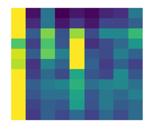
To appreciate the concept of SHAP values, it is instructive to consider correlation matrices of the training data as shown in figure 8(a,b) for classes 0 and 1, respectively. A few observations can be made from the data. First, the correlation matrices belonging to two classes are remarkably similar, demonstrating that correlations alone are not sufficient to distinguish between the classes. Here, we note that correlations only capture linear relations between random variables. The only difference is that modes 4 and 5 positively correlate in class 0, while they correlate negatively in class 1, and similarly for modes 7 and 8. When comparing the correlation matrices with the mode coupling table or with the amplitude equations in Moehlis et al. (Reference Moehlis, Faisst and Eckhardt2004) we observe that strongly correlating modes couple via either the laminar profile (mode 1) or its deviation in streamwise direction (mode 9). The strong negative correlations between modes 2 and 3, and strong positive correlations between modes 6 and 7, which occur for both classes, can be made plausible by inspection of the evolution equation of the laminar profile. The nonlinear coupling only extract energy from the laminar flow if the amplitudes of modes 2 and 3 have the opposite sign, and those of modes 6 and 8 are of the same sign as products of these mode pairs occur in the evolution equation of the laminar profile. In other words, in order to obtain an unsteady dynamics, modes 2 and 3 must be mostly of opposite sign while 6 and 8 must mostly have the same sign. In this context we note that the amplitude of the laminar mode is always positive, as can be seen from figure 2(a).

Figure 8. (a,b) Correlation matrices of training data for classes 0 and 1, respectively. Class  $1$ (
$1$ ( $0$) corresponds to samples that do (not) relaminarise after $t_p$ time steps. (c,d) Mean absolute SHAP interaction values of the first $N_v/10=10\,000$ validation samples for classes 0 and 1, respectively. As self-correlations encoded in the diagonal elements do not convey useful information, the diagonal elements have been set to zero for all panels for presentational purposes.
Secondly, we consistently find correlations between modes identified as significant for the prediction and irrelevant modes. For instance, modes one and nine correlate, and so do mode two and three, four and five. Thirdly, modes that are considered significant do not correlate. The latter two points highlight the game-theoretic structure of SHAP. For example, as the fluctuations of the coefficients pertaining to modes two and three are strongly correlated, it is sufficient for the classifier to know about one of them. We will return to this point in § 4.3.
To elucidate second-order interaction effects further, the SHAP interaction values (Lundberg et al. Reference Lundberg, Erion, Chen, DeGrave, Prutkin, Nair, Katz, Himmelfarb, Bansal and Lee2020) are computed, see figure 8(c,d). The overall bar heights denote the mode importance across both classes, the coloured bars distinguish between both classes. Interactions between modes  $3$ and $5$ are found to be strongest for samples from both prediction classes. In particular modes $7$ and $8$ differ in their importances for the two classes: both are more important in cases where relaminarisation does not occur. Interaction effects between modes $4$ and $5$ are present for both classes, but more pronounced for samples of class $0$. Generally, interaction effects of samples of class $1$ are stronger than for those of class $0$.
$0$.
The feature importances presented in figure 7 show that the laminar mode is consistently identified as a relevant feature. The shortest prediction time  $t_p=200$ not only comes with a prediction accuracy of ${\approx }98\,\%$, but the feature importance of the laminar mode is also significantly stronger than for the other tested prediction horizons. This indicates that this prediction case can, indeed, be considered a validation case. Within that scope, the validation succeeded as the statistically significant laminar mode is detected as most relevant mode.
Increasing the prediction horizons leads to a decrease in the importance metric for all features, as can be inferred from the observed decrease in normalisation factors shown in figure 7(b). The normalisation constants shown in figure 7(b) are computed as  $N_i=\sum _{j=1}^{9} \varPhi _{i,j}$, where $\varPhi _{i,j}\in \mathbb {R}$ denotes the SHAP value of mode $j \in \{1, \ldots, 9\}$ for a prediction time $t_p^{(i)}$, the superscript $i$ enumerating the sampled prediction times $t_p \in \{200, 225, \ldots, 450\}$. Figure 7(a) thus presents $\varPhi _{i,j}/N_i$. The observed decrease in normalisation factors with increasing $t_p$ indicates, together with declining prediction performance, that sufficiently well-performing classifiers are required to enable the subsequent explanation step.
4.3. Interpretation
Throughout the prediction horizons,  $\boldsymbol {u}_1$, $\boldsymbol {u}_3$ and $\boldsymbol {u}_5$ are consistently considered important. These modes represent the laminar profile, the streamwise vortex and a spanwise sinusoidal linear instability of the streak mode $\boldsymbol {u}_2$, respectively. Streamwise vortices and streaks are a characteristic feature of wall-bounded shear flows (Hamilton, Kim & Waleffe Reference Hamilton, Kim and Waleffe1995; Bottin et al. Reference Bottin, Daviaud, Manneville and Dauchot1998; Schmid, Henningson & Jankowski Reference Schmid, Henningson and Jankowski2002; Holmes et al. Reference Holmes, Lumley, Berkooz and Rowley2012). Alongside the laminar profile its linear instabilities $\boldsymbol {u}_4$– $\boldsymbol {u}_7$, they play a central role in the self-sustaining process, the basic mechanism sustaining turbulence in wall-bounded shear flows. The importance of the streamwise vortex $\boldsymbol {u}_3$ increases with prediction horizon and decreases from $t_p\approx 300$ onwards, where the prediction accuracy begins to fall below $90\,\%$.
The streak mode itself appears to be irrelevant for any of the predictions, which is remarkable as it is, like the streamwise vortex, a representative feature of near-wall turbulence. Similarly, its instabilities, except mode  $\boldsymbol {u}_5$, are not of importance for the classification. For the shortest prediction time, that is, for the validation case $t_p = 200$, mode $\boldsymbol {u}_5$ does not play a decisive role either, which is plausibly related to the SSP being significantly weakened close to a relaminarisation event. This rationale, of course, only applies to data samples in class 1, where relaminarisation occurs. Like the vortex mode $\boldsymbol {u}_3$, the spanwise instability mode $\boldsymbol {u}_5$ increases in importance with prediction horizon except for the longest prediction horizon, which again can be plausibly explained by a more vigorous SSP further away from a relaminarisation event. Since $\boldsymbol {u}_1$ and $\boldsymbol {u}_3$ are translation invariant in the streamwise direction, a mode with $x$-dependence should always be recognised, as the SSP cannot be maintained in two dimensions. The dominance of $\boldsymbol {u}_5$ over any of the other instabilities may be related to its geometry resulting in a stronger shearing and thus a faster instability of the streak.
Apart from modes directly connected with the SSP, the deviation of the mean profile from the laminar flow,  $\boldsymbol {u}_9$, is also recognised as important for $t_p = 200$ and $t_p = 250$. Turbulent velocity field fluctuations are known to alter the mean profile. In extended domains, where turbulence close to its onset occurs in a localised manner, localisation occurs through turbulence interacting with and changing the mean profile. The mean profile of a puff in pipe flow, for instance, is flatter than the Hagen–Poiseuille profile towards the middle of the domain, which decreases turbulence production (van Doorne & Westerweel Reference van Doorne and Westerweel2009; Hof et al. Reference Hof, de Lozar, Avila, Tu and Schneider2010; Barkley Reference Barkley2016).
Now the question arises as to if and how the information SHAP provides concerning the mode importance ranking can be connected to the equations of motion and what can be learned from this. In particular, concerning strongly correlated modes, it is instructive to understand why a particular mode is favoured. For modes two and three, the mode coupling table of Moehlis et al. (Reference Moehlis, Faisst and Eckhardt2004) again gives some indications. Mode three (the streamwise vortex) generates mode two (the streak) by advection of mode one (the laminar profile) – this is the first step of the SSP – or mode 9 (the deviation of the laminar profile). However, the coupling table is not symmetric, that is,  $\boldsymbol {u}_2$ cannot generate $\boldsymbol {u}_3$, and $\boldsymbol {u}_3$ can only be re-generated through nonlinear interactions involving either $\boldsymbol {u}_5$ and $\boldsymbol {u}_6$ or modes $\boldsymbol {u}_4$ and $\boldsymbol {u}_7$ or $\boldsymbol {u}_8$ – this is known as the third and last step in the SSP, where instabilities couple nonlinearly to re-generate the streamwise vortex. Hence, out of the strongly correlated mode pair $\boldsymbol {u}_2$ and $\boldsymbol {u}_3$, the latter should be physically more significant in the SSP than the former, in the sense that $\boldsymbol {u}_2$ will become active if $\boldsymbol {u}_1$ and $\boldsymbol {u}_3$ are, but not vice versa. SHAP indeed identifies $\boldsymbol {u}_3$ as significant while $\boldsymbol {u}_2$ plays no decisive role in the prediction. A similar conclusion has recently been obtain for the transition to turbulence in flow through a vertically heated pipe (Marensi, He & Willis Reference Marensi, He and Willis2021), where relaminarisation due to buoyancy forces has been connected with a suppression of streamwise vortices rather than streaks.
For modes 4 and 5 the situation is more subtle, as both modes can be converted into each other through advection by the laminar profile. Again considering the mode coupling table (or the amplitude equations), two points distinguish mode 5 from mode 4: (a) mode 5 is odd in  $x_2$ while mode 4 is even in $x_2$, (b) in interactions with mode 2, mode 5 couples to the only fully 3d mode, mode 8 (which is also odd in $x_2$), while mode 4 does not. A fully fledged SSP should involve three-dimensional dynamics, and the data distribution of mode 8 shows this clearly for the validation case ( $t_p = 200$) as mode 8 is significantly weakened in class 1 compared with class 0. Considering the training data distributions of modes 4, 5 and 8, we observe that the probability density functions (p.d.f.s) of mode 5 differ considerably between class 0 and class 1, and again mode 5 is suppressed in class 1. In contrast, mode 4 is active in both classes. Mode 5 thus provides a more direct route to a three-dimensional dynamics from streak instabilities than mode 4 does.
In summary, the picture that emerges is as follows. For a sustained SSP, the streamwise vortex must be remain active as only it can generate the streak. Further to this, supplying spanwise flow perturbations of odd parity in wall-normal direction should help to prevent relaminarisation events, while spanwise flow fluctuations connected with streak instabilities of even parity in wall-normal direction play a minor role in sustaining the SSP.
5. Example – SHAP on data obtained by DNS
In order to demonstrate that the method can be leveraged to larger fluid dynamics datasets, we now discuss an example where SHAP values corresponding to the prediction of relaminarisation events are calculated on a dataset obtained by DNS of minimal plane Couette flow at transitional Reynolds number. For this particular example, features are not tied to physical processes or any modal representation of the flow. Instead, the analysis is carried out on flow-field samples, and SHAP is used in conjunction with a now NN-based classifier to provide (a) an indication as to which flow features need to be observed to allow an accurate prediction of relaminarisation events, and (b) an interpretation thereof in terms of the SSP. Specifically to address the latter and to connect to the results obtained for the SSP within the NMM, we ask the classifier to predict relaminarisation events based on the structure of the streaks characteristic for the SSP, and we use SHAP to demonstrate that the classifier bases its decisions on data features indicating the presence of streak instabilities. To do so, we focus on the streamwise component of the velocity field evaluated at a particular point in streamwise direction, that is, the classifier works with two-dimensional data slices showing cross-sections of high- and low-speed streaks.
5.1. Numerical experiments
In order to keep the computational effort to a manageable level commensurate with an example calculation, we consider simulations of plane Couette flow at a Reynolds number of 400 in the minimal flow unit, a domain of size  $L_1\times L_2 \times L_3 =1.755{\rm \pi} \times 2 \times 1.2{\rm \pi}$ with periodic boundary conditions in the streamwise and spanwise directions and no-slip boundary conditions in the wall-normal direction, the smallest domain that sustains turbulence (Jiménez & Moin Reference Jiménez and Moin1991; Hamilton et al. Reference Hamilton, Kim and Waleffe1995; Kawahara & Kida Reference Kawahara and Kida2001). The calculations have been carried out with a pseudospectral solver provided by channelflow2.0 (Gibson Reference Gibson2014; Gibson et al. Reference Gibson2022) using $n_1 \times n_2 \times n_3 = 16 \times 33 \times 16$ points in the streamwise, wall-normal and spanwise directions, respectively, with full dealiasing in the streamwise and spanwise directions, a resolution similar to other, including recent, studies of minimal plane Couette flow (Kawahara & Kida Reference Kawahara and Kida2001; van Veen & Kawahara Reference van Veen and Kawahara2011; Lustro et al. Reference Lustro, Kawahara, van Veen, Shimizu and Kokubu2019). We generate velocity field data for $5000$ trajectories running for $5000$ advective time units and take data samples at an interval of 10 advective time units. The simulations are initialised with randomly perturbed velocity-field samples taken at intervals of one advective time unit from a turbulent master trajectory and the training data acquisition process is started after a transient of 100 advective time units. The criterion for the observation of a relaminarisation event is a cross-flow energy threshold of $10^{-5}$, and we verify that the turbulent lifetime distribution is still exponential for this grid size (not shown).
As indicated earlier, a convolutional NN is trained on the streamwise slice at  $x_1=0$ of the streamwise $u_1$ component with around $5000$ samples, yielding a spatial sample size of $10 \times 33$, taking into account truncation to remove aliasing effects. Two two-dimensional convolutional layers with subsequent two-dimensional max pooling layers are followed by a flattening layer with a dropout layer and a fully connected softmax layer with two neurons, one for each output class (Chollet Reference Chollet2021), to establish the NN graph. The size of the snapshots is well within the capabilities of NNs, that is, the method can certainly be applied to higher-resolved data. The main reason for the choice of resolution here is that the exponential lifetime distribution results in having to discard a significant number of trajectories, essentially all those where relaminarisation occurred very quickly, in order to ensure that the transient from the initial data has passed. After training the NN, the SHAP values for samples from the test dataset are calculated. We can focus on the SHAP values for class $1$ only, as the SHAP values for the two classes differ only by a minus sign.
5.2. Results
First, the prediction time  $t_p$ is varied between $10$ and $200$ advective time units to obtain the performance of the convolutional network for tasks of different difficulties (Lellep et al. Reference Lellep, Prexl, Linkmann and Eckhardt2020). The performance decreases from approximately $99\,\%$ prediction accuracy for $t_p<60$ to approximately $60\,\%$ at $t_p=200$ with a performance $>90\,\%$ for $t_p \leq 130$ (not shown). In what follows, we discuss results obtained for $t_p = 90$, however, results are consistent with larger prediction horizons with a prediction accuracy of ${>}90\,\%$. In figure 9 we present one representative sample for each of the two classes together with the spatial distribution of SHAP values to illustrate general observations that can be obtained from the data.

Figure 9. Two representative velocity-field samples (top) and corresponding SHAP values (bottom) for (a) class  $0$ and (b) class $1$. For the velocity field, streak cross-sections, that is the deviation of the streamwise velocity component from the laminar profile evaluated at $x_1 = 0$ is shown. As can be seen by comparison of the top and bottom panels, SHAP uses streak tails, that is regions where the streaks are spatially decaying, for classification towards class $1$ and streak cores, where the velocity is nearly uniform, for classification towards class $0$.
$0$.
The streamwise component  $u_1$ of velocity-field samples evaluated at $x_1 = 0$ always consists of localised regions in the velocity field of alternating small and large magnitudes, corresponding to cross-sections of low- and high-speed streaks. Samples corresponding to class $0$ feature less uniform streak cross-sections than those of class $1$. More precisely, the spatial decay of a streak in the wall-normal and spanwise directions is less regular for samples of class $0$ than for those of class $1$. This can be seen by comparison of the representative visualisations shown in figure 9(a) for class $0$ and figure 9(b) for class $1$. In what follows, we refer to regions of spatial decay as streak tails.
For samples of class  $0$, i.e. those that do not relaminarise, the SHAP values are mostly negative while the SHAP values for samples of class $1$ are mostly positive. Furthermore, for samples of class $0$ SHAP values detect the streak cores, where $u_1$ varies little, more so for the low-speed rather than the high-speed streak. For class $1$, however, the SHAP values point towards the tails of the corresponding more uniform streak cross-sections. The tails of the high-speed streaks are more pronounced. Interestingly, the tails of the less regular class- $0$ streak cross-sections slightly contribute towards a classification of those samples to class $1$ and the inner region of the class- $1$ small velocity regions contribute to the classification of those samples to class $0$. That is because the tails and the core look similar to those of the other class, respectively. We can therefore conclude that the NN uses the streak cores for the classification towards class $0$ and the streak tails, where velocity-field gradients are large, for the classification towards class $1$.
$1$.
5.3. Discussion
The two-dimensional slices used in the training result in the classifier having to predict relaminarisation events based on the structure of the streaks, but without directly seeing the streak modulations characteristic of linear streak instabilities, as these would only be visible in either the full volume or in a wall-normal cross-section of the flow. Comparing wall-normal cross-sections obtained from samples of classes 0 and 1 a posteriori, we find consistently that streak modulations are much weaker or absent in class 1 compared with class 0. In conjunction with the results obtained by SHAP, we conclude that the classifier bases its decision on proxies for streak modulations corresponding to linear streak instabilities within the SSP.
For a relaminarisation event to occur, the SSP must break at some point in its evolution. The SSP consists of three consecutive stages, (i) the laminar profile is advected by the streamwise vortex creating streaks, (ii) the streaks become linearly unstable, (iii) the linear instabilities couple nonlinearly and re-generate the streamwise vortex. Relaminarisation could in principle be related with any of these stages, for instance, with a weakening of streaks or of streamwise vortices or a suppression of streak instabilities. Strong streaks are present in both class 0 and class 1 DNS data samples, as can be seen from the visualisations of representative data samples shown in figure 9. This is commensurate with the results obtained for the NMM, where we found that the streak mode itself is not relevant for the prediction of relaminarisation events. That is, a scenario whereby relaminarisation is connected with a suppression of streaks is unlikely. A similar observation has been made for buoyancy-induced relaminarisation in a vertically heated pipe (Marensi et al. Reference Marensi, He and Willis2021). In contrast to this, and as discussed above, accurate predictions of relaminarisation events can be made based on the presence or absence for proxies for linear streak instabilities. If they are present, the streaks have a less regular profile and the flow remains turbulent, if not, it relaminarises. We note that the classification task did not involve observables connected with streamwise vortices. However, as streamwise vortices are a consequence of streak instabilities, not precursors, a suppression of streak instabilities would necessarily result in a suppression of streamwise vortices. In summary, the SHAP analysis suggests that the break-up point in the self-sustaining cycle is connected with a suppression of streak instabilities.
Using two-dimensional slices of a low-resolution DNS near the laminar–turbulent transition as training data for relaminarisation, predictions shows that SHAP values yield insights into what is important for the prediction in the demonstration carried out here. Specifically, localised SHAP values can be linked to localised coherent regions of the flow, thereby providing a way to find relevant flow features for what the convolutional NN classifier uses for the prediction. Interestingly, regions where velocity-field gradients are large, that is, the tail ends of the streak cross-sections play a major role in the prediction of relaminarisation events.
The ability of SHAP to identify localised regions in the flow and isolate important sub-regions therein suggests that SHAP values can also identify physical processes that are used by classifiers provided a data representation capable of encoding physical, i.e. dynamical, processes is used. This would involve passing temporally resolved data, for instance by providing single training samples consisting of time-ordered data samples in sub-intervals of a given time series. Additionally, the correlation between input data and relevance for classifiers as determined by SHAP values could be used by experimentalists to, for instance, increase measurement resolution where necessary or optimise the location of probes.
6. Conclusions
The purpose of this article is to introduce SHAP as an explainable AI method capable of identifying flow features relevant for the prediction of relaminarisation events in wall-bounded parallel shear flows. As a first step and in order to facilitate a physical interpretation of the SHAP output, we used a dataset consisting of snapshots generated through forward integrations of the NMM of Moehlis et al. (Reference Moehlis, Faisst and Eckhardt2004), as it is based on the SSP and each feature, here corresponding to a basis function, has a clear physical meaning. Subsequently, the same classification task is carried out on data obtained from DNSs of minimal plane Couette flow, where we specifically focus on the prediction of relaminarisation event based on the structure of high- and low-speed streaks. The feature ranking furnished by SHAP was interpreted in the context of the SSP, resulting in a clear distinction between those near-wall features phenomenologically representative of the flow and those significant for the dynamics of a wall-bounded turbulent flow close to the onset of turbulence. More specifically, we demonstrated that relaminarisation events are preceded by a weakening of streak instabilities and thus necessarily of streamwise vortices, rather than being connected with the streaks themselves. Relaminarisation can only occur when the self-sustaining cycle breaks up, and our analysis suggests that this happens at the streak instability stage.
Concerning the NMM, each data feature has a clear physical interpretation. This allows us to address the issue of representativeness vs significance (Jiménez Reference Jiménez2018). To do so, we suggest to classify the information obtained into two categories, one comprises features of known phenomenological importance – the representative features – which can be identified in a shear flow by the naked eye such as streamwise vortices or streaks, and the other comprises features of potential dynamical significance that are more difficult to observe directly, i.e. being not or at least much less representative. In the present context, the second class contains modes representing linear streak instabilities, for instance. For the first class, SHAP was used to uncover which of the known representative features were significant for the prediction of relaminarisation events. First, we see that a known representative feature of near-wall dynamics, the streamwise vortex, is identified. Second, and more interestingly, the dynamics of streak mode, also a representative feature, is not relevant for the prediction of relaminarisation events. In the second class, SHAP identifies a dynamically significant feature among the streak instabilities, the fundamental spanwise mode that is odd in  $x_2$. This suggests that, even though the streak has several types of instabilities within the SSP, the main effect on the dynamics with respect to relaminarisation events stems from spanwise instabilities of odd parity with respect to reflection about the midplane, at least in the NMM.
For the DNS data, we find that SHAP identifies spatially localised regions in the flow that are relevant for the prediction of relaminarisation events. Taking guidance from the results obtained for the NMM, a classification task to probe the relevance of streak instabilities for the prediction of relaminarisation events was constructed by showing two-dimensional data planes orthogonal to the spanwise direction to a classifier, that is, planes including cross-sections of high- and low-speed streaks. We find that SHAP values cluster in certain regions on the plane connected with variations in streak structure, which indicates that the classifier bases its decision on proxies for streak modulations corresponding to linear streak instabilities within the SSP. Since streamwise vortices are generated by nonlinear interactions of streak instabilities, SHAP thus identifies the suppression of streak instabilities as the point of breakdown within the self-sustaining cycle leading to relaminarisation.
SHAP thus identifies not only which of the characteristic phenomenological features of the SSP in a wall-bounded shear flow are significant for the prediction of relaminarisation events, it also recognises patterns in the data corresponding to its fundamental dynamical mechanism. That is, it serves as a means to distinguish representativeness from significance of features for a given ML task. Furthermore, variances in the feature importance ranking across prediction horizons are commensurate with differences in the dynamics one would expect closer or further away from a relaminarisation event.
Finally, we conclude with a few suggestions for further work. As SHAP is model agnostic and can be used in conjunction with deep learning algorithms, this method can be upscaled and applied to high-dimensional experimental and numerical data. Essentially, we can envisage two main application categories, one aimed at obtaining further physics insight from high-dimensional numerical or experimental data, and one at purely technical improvements of analysis routines. The former will in most instances require a pre-processing step to decompose the data into physically interpretable features, while no such decomposition would be required for the latter to yield useful results. The results for the low-dimensional model presented here serve as a proof of concept for the former. The aforementioned example calculation using DNS data of transitional minimal plane Couette flow, where SHAP was used to identify regions in the flow that the classifier needs to see in order to render accurate predictions, demonstrates that the latter is in principle possible. An in-depth analysis of DNS data at higher Reynolds number and resolution is beyond the scope of the present paper, however, it would be a very interesting follow-up study. For the former, examples for useful data decompositions are proper orthogonal decomposition (POD) (Berkooz, Holmes & Lumley Reference Berkooz, Holmes and Lumley1993) or dynamic mode decomposition (DMD) (Schmid Reference Schmid2010), both by now widely used techniques for data analysis and model reduction in fluid dynamics. While POD returns modes corresponding to energy content, DMD decomposes experimental or numerical data into spatio-temporally coherent structures labelled by frequency. The suitability of any data decomposition and reduction technique would depend on the planned task.
Identifying important modes and their interactions for a data representation without a straightforward physical interpretation could be useful to construct, for instance, a lower-dimensional description of the dynamics by only retaining important modes for any given ML task at hand. In complex geometries, SHAP analyses could provide guidance as to which part of a simulation domain requires high resolution and where compromises regarding resolution and simulation cost will be less detrimental to the overall accuracy of the simulation. This can become particularly helpful with pure turbulence research, such as for active fluids, geo- and astrophysical flows, viscoelastic flows or complex flow geometries, as these applications are data intensive and the flow complexity often does not allow straightforward feature interpretation.
Ultimately, results reported here are based on a statistical analysis of the SHAP values. Additionally, as SHAP values can be calculated alongside real-time predictions, per-sample SHAP values may prove themselves as useful tools in on-the-fly tasks such as machine-assisted nonlinear flow control or for optimisation problems.
Acknowledgements
This project originated through discussions with B. Eckhardt, who sadly passed away on August 7th 2019. We hope to have continued the work according to his standards and any shortcomings should be attributed to M. Linkmann. The authors thank T. Bischoff, M. Buzzicotti, P. Veto, M. Grau, X. Zhu, B. Noack, E. Jelli and J. Schumacher for helpful conversations. The computations have been carried out on the MaRC2 compute cluster of the Philipps-University of Marburg and on Cirrus (www.cirrus.ac.uk) at the University of Edinburgh. We thank the respective support teams for technical advice. Computing time on Cirrus was provided through a Scottish Academic Access allocation.
Funding
We acknowledge financial support from the German Academic Scholarship Foundation (Studienstiftung des deutschen Volkes) and the Priority Programme SPP 1881 ‘Turbulent Superstructures’ of the Deutsche Forschungsgemeinschaft (DFG) under grant Li3694/1.
Declaration of interests
The authors report no conflict of interest.
Data availability statement
The data for this study are publicly available at https://doi.org/10.7488/ds/3450.
Appendix A
A.1. Boosted trees
In boosted methods, the ensemble of  $K$ weak learners, $\{g_k\}_{k=1}^{K}$, is set up in an additive manner, so that the output of the boosted model $g^{(K)}$ for a sample $\boldsymbol {z}\in \mathbb {R}^{M}$ is
 \begin{equation} g^{(K)}(\boldsymbol{z}) = \sum_{k=1}^{K} g_k(\boldsymbol{z})\in\mathbb{R}. \end{equation}
The models  $g_k$ are learned sequentially so as to correct the mistakes of the previous models $\{g_i\}_{i=1, \ldots, k-1}$ without altering them. Given a per-sample loss $L(\kern0.5pt y, \hat {y})$ between the true sample label $y$ and the prediction of the previous model $\hat {y}=g^{(k-1)}$, the next weak learner $g_k$ is found by optimising
 \begin{equation} \min_{g_k} \sum_{n=1}^{N_t} L(\kern0.5pt y_n, g^{(k-1)}(\boldsymbol{z}_n)+g_{k}(\boldsymbol{z}_n)), \end{equation}
with  $N_t$ as number of training samples.
Boosted trees use decision trees  $T(\boldsymbol {z}; \boldsymbol {\theta })$ (Breiman et al. Reference Breiman, Friedman, Stone and Olshen1984) as weak learners, $g_k(\boldsymbol {z}) = T(\boldsymbol {z}; \boldsymbol {\theta })$ with $\boldsymbol {\theta }$ as parameters of the decision tree. A decision tree classifier is a binary tree that categorises its input as the class of the terminal node the input is assigned to. A decision tree with $J$ terminal nodes evaluates $T(\boldsymbol {z}; \boldsymbol {\theta })$ according to
 \begin{equation} T(\boldsymbol{z}; \boldsymbol{\theta}) = \sum_{j=1}^{J} \gamma_j I(\boldsymbol{z}\in R_j), \end{equation}
with  $I$ as indicator function and parameters $\boldsymbol {\theta }=\{R_j, \gamma _j\}_{j=1}^{J}$ as terminal regions $R_j$ of the terminal nodes in the input space and the assigned values in the terminal nodes $\gamma _j$.
Figure 10 illustrates how a spectral velocity field is classified according to an example decision tree with  $J=3$. The sample we seek to classify is assigned to the grey terminal node with a dashed border after it transverses the binary tree structure. The structure is made up of binary decisions, which are noted next to the nodes in black. The predicted class of the sample is 1, since the terminal node it has been assigned to is itself assigned the class 1. Learning a tree consists of finding the appropriate tree structure and the terminal node classes in grey.

Figure 10. Schematic classification of a spectral velocity field  $\boldsymbol {a}$ by a decision tree. The dotted and dashed lines denote positive and negative decisions, respectively. The $J=3$ terminal notes are coloured in grey and the dashed terminal node marks the output of the example classification.
Boosted trees have been shown to yield state-of-the-art performances on a number of standard classification benchmarks (Li Reference Li2010) and are thereby suitable for the task of classifying relaminarisation events in shear flows.
As finding the optimal tree structure is an intractable problem, gradient boosted trees make use of the gradient of the deployed per-sample loss function  $L$ for finding an optimal tree structure $\{R_j\}_{j=1}^{J}$. The specific role of the gradients in improving the boosted trees depends on the exact model: for example, traditional gradient boosted tree methods (Ridgeway Reference Ridgeway2006) fit a decision tree to the negative gradient of $L$, arising from the first-order Taylor expansion of (A 2), in order to benefit from the generalisation ability of the tree to new data (Hastie et al. Reference Hastie, Tibshirani and Friedman2009, Chapter 10.10).
The gradient boosted tree algorithm implemented by XGBoost, however, extends the boosting objective (A 2) about a regularisation term and expands the loss function  $\mathcal {L}^{(k)}$ in the next weak learner $g_k$ to be added
 \begin{align} \mathcal{L}^{(k)} &= \sum_{n=1}^{N_t} L(\kern0.5pt y_n, \hat{y}_{n}^{(k-1)}+g_k(\boldsymbol{z}_n)) + \varOmega(g_k) \nonumber\\ &\approx \sum_{n=1}^{N_t} \left[L(\kern0.5pt y_n, \hat{y}_n^{(k-1)})+ \left.\frac{\partial L(\kern0.5pt y_n, d)}{\partial d}\right|_{d=\hat{y}_n^{(k-1)}}g_k(\boldsymbol{z}_n) \right.\nonumber\\ &\quad +\left.\frac{1}{2} \left.\frac{\partial^{2} L(\kern0.5pt y_n, d)}{\partial d^{2}}\right|_{d=\hat{y}_n^{(k-1)}} g_k^{2}(\boldsymbol{z}_n)\right] + \varOmega(g_k) , \end{align}
as iterative objective for iteration step  $k$ with regularisation $\varOmega (g_k)=\omega J_k + \frac {1}{2} \lambda |(\gamma _{1k}, \ldots, \gamma _{J_k k})|^{2}$ on tree $k$. Here, $J_k$ denotes the number of terminal nodes of tree $k$ and $\gamma _{jk}$ with $j=1,\ldots,J_k$ is the terminal node weight of index $j$ and tree $k$. Using $R_{jk}$ as terminal node set of index $j$ and tree $k$, the objective is used to quantify the quality of a tree structure after minimising the quadratic iterative objective
 \begin{equation} \mathcal{L}^{(k)}(\{R_{jk}\}_{j=1,\ldots,J_k}) ={-}\frac{1}{2}\sum_{j=1}^{J_k} \frac{\left(\displaystyle\sum_{i\in I_j}h_i^{(1)}\right)^{2}}{\displaystyle\sum_{i\in I_j}h_i^{(2)} + \lambda}+\omega J_k, \end{equation}
with  $I_j=\{i\,|\,q(\boldsymbol {z}_i)=j\}$ as terminal node index set, $q(\boldsymbol {z})$ mapping a sample to the index of the terminal node it is assigned to and $h^{(1)}$ and $h^{(2)}$ as first- and second-order derivatives of $L$ from (A 4), respectively. Using $\mathcal {L}^{(k)}(\{R_{jk}\}_{j=1,\ldots,J_k})$, the quality of a node $I$ to be split into left and right, $I=I_L\cup I_R$, can be measured quantitatively.
The remarkable novelty of XGBoost, aside from the regularisation  $\varOmega (g_k)$, is a split finding technique that uses weighted data quantiles to find appropriate split candidates, which are themselves evaluated with a novel approximate split finding algorithm that uses the split loss $\mathcal {L}^{(k)}(\{R_{jk}\}_{j=1,\ldots,J})$ as metric. Furthermore, XGBoost scales to very large datasets as all components are properly parallelisable. This is due to additional technical innovations, such as data sparsity awareness, cache awareness and out-of-core computations if the dataset gets very large.
The loss function  $L$ is the logistic regression for binary classification with output probabilities
 \begin{equation} L(\kern0.5pt y, \hat{y}) = y \log(\sigma(\hat{y})) + (1-y) \log(1-\sigma(\hat{y})), \end{equation}
with logistic function  $\sigma (\kern0.5pt y)=1/(1+\exp (-y))$.
XGBoost classifiers come with a number of tuneable hyperparameter that need to be specified by the user. The following parameters are tuned in this work and are therefore explained here using the XGBoost notation:

A.2. Optimal XGBoost hyperparameters for relaminarisation prediction
Table 1 lists the optimal hyperparameters as identified by the randomised hyperparameter optimisation with  $100$ drawn hyperparameter samples. Since all prediction times use the same $100$ hyperparameter samples, the same set of hyperparameters might be found to be optimal for more than one prediction horizon, e.g. $t_{p}=200$ and $250$.
Table 1. Table of optimal hyperparameters for XGBoost classifier for the task of predicting the relaminarisation of the turbulent trajectory. The abbreviations in the header line have been introduced in the main text of Appendix A.1.


 Open access