1 INTRODUCTION
Though the primary aim of the KEPLER Mission was to discover Earth-like planets around other stars, the high-precision and continuous photometric data also enable us to make a significant breakthrough in stellar astrophysics. From the discovery of ‘heart-beat’ binaries (Thompson et al. Reference Thompson2012) to the asteroseismology studies, KEPLER data considerably enlighten our knowledge of astrophysics. Eclipsing binary stars on the other hand, are known as one of the best laboratories, by which we can measure absolute parameters (e.g., masses and radii) allowing us to test the stellar structure and evolutionary models. Therefore, it is inevitable that the simultaneous analyses of KEPLER light curves with radial velocity data provide us to obtain the absolute parameters with incomparable accuracy.
Amongst the absolute parameters of eclipsing binary stars, mass ratio (q = M 2/M 1) is the key parameter especially in studying the close binary evolution. As mentioned by Rucinski (Reference Rucinski2001), the ‘correct’ way to determine the mass ratio is based on radial velocity observations, by which one can determine the q sp parameter from the ratio of velocity semi-amplitudes (q = M 2/M 1 = K 1/K 2) of both components. The other way, which is somewhat controversial, is the determination of the mass ratio from light curve analysis alone. This quantity is usually denoted as q ph.
The quantity q ph and its reliability have been discussed by many authors throughout the years. The first applications of q ph to the W UMa type overcontact binaries with total eclipses were performed by Mochnacki & Doughty (Reference Mochnacki and Doughty1972a, Reference Mochnacki and Doughty1972b) whereas the first concrete explanation regarding why q ph is reliable in case of overcontact binaries showing total eclipses was made by Wilson (Reference Wilson1978). The main point is that, in order for q ph to be accurate (i.e., q ph = q sp), certain constraints need to be applied so that the range of possible values of mass ratio be significantly reduced. If a star fills its Roche lobe, then the star size determines the lobe size relative to mass ratio, at least for the synchronous rotation case (Wilson Reference Wilson1994). The work of Terrell & Wilson (Reference Terrell and Wilson2005) performed with synthetic data can be regarded as a cornerstone in this manner. In this work, it has been shown that a steep relation exists between the ratio of the radii (r 1/r 2, where r 1, 2 = R 1, 2/a represent the fractional radii) and the mass ratio for overcontact binaries. According to this study, for the overcontact binaries of the W UMa-type with total eclipses, orbital inclination does not have any effect on the eclipse depths and since the surface brightnesses of the components are nearly the same for W UMa’s, eclipse depths are determined by fractional area covered during eclipses, which gives the ratio of the radii. Combining these results with the Roche geometry for W UMa-type systems, which requires the surface potentials of the components be equal, the range of possible q values is greatly reduced (Terrell & Wilson Reference Terrell and Wilson2005). The result is therefore given as photometric mass determination can yield reliable results for W UMa-type systems having total eclipses.
As for the semi-detached case, where only one component fills its Roche lobe, there is also a steep relation between the mass ratio and the fractional side radius of the lobe-filling component, thus, making it possible to determine accurate photometric mass ratios in case of total eclipses (Terrell & Wilson Reference Terrell and Wilson2005). When comparing q sp (namely the real value of the mass ratio) with q ph, it has been seen that there is a good agreement between q sp and q ph for totally eclipsing overcontact and semi-detached systems but as for the partial eclipsing systems, the relation between q sp and q ph gets worse, the reason of which is thought to be the missing radii information in case of partial eclipses (Terrell & Wilson Reference Terrell and Wilson2005). However, despite these crucial results, q ph method is still frequently used for partially eclipsing binaries in the literature, resulting in questionable results.
In the work of Hambálek & Pribulla (Reference Hambálek and Pribulla2013), it has been stated that in the presence of third light (l 3), q ph will be erroneous since q anti-correlates with third light. They also confirmed the results given by Terrell & Wilson (Reference Terrell and Wilson2005) stating that q ph is reliable in the case of totally eclipsing overcontact and semi-detached systems and added that the range of possible values of q decreases, whereas the amplitude of the light curve increases.
In the light of these conclusions, we aim to determine the photometric mass ratios of W UMa type KEPLER eclipsing binaries exhibiting total eclipses, compare them with the spectroscopic mass ratios for the systems which radial velocity observations are available, then perform the analyses of their light curves, and finally estimate their absolute parameters using some approximations.
2 KEPLER DATA
The sample selection was performed via the KEPLER Eclipsing Binary CatalogFootnote 1 , formed following the work of Prša et al. (Reference Prša2011). Every input in the catalogue was checked in order to find systems showing total eclipses. We paid attention to select systems whose maximum light levels (at the quadrature phases) are the same or at least very close to each other, i.e., systems having no or very little O’Connell effect. The list of the selected targets and some of their parameters taken from the catalogue are given in Table 1.
Table 1. List of some parameters of W UMa type eclipsing binaries with total eclipses taken into account within the context of this study.

a Depth of the primary minimum calculated after obtaining normalised light curve.
After the selection of the systems, we retrieved the actual long cadence data from MAST (Mikulski Archive for Space Telescopes)Footnote 2 as fits files which contain the SAP (Simple Aperture Photometry) flux values for each quarter . The cotrending or detrending processes (removal of systematic trends and features) of the data were performed via pyke Footnote 3 software (Still & Barclay Reference Still and Barclay2012). According to the recommendation of the software publishers that the cotrending process was preferable to the detrending process for most of the KEPLER targets, we performed cotrending with CBV (Cotrending Basis Vectors) files providedFootnote 4 . An example of the cotrending process is given in Figure 1. For each system, after cotrending or detrending, light curves available in all quarters were merged. Then, scattered points in the merged light curves of each system were rejected, according to 1-σ criterion, using an IDL code so that clean light curves were acquired, as shown in Figure 2. Finally, light curves with normal points and normalised to the maximum light level were acquired (Figure 2) and the rest of the work was performed on these final light curves.

Figure 1. An example of the cotrending process via pyke for the quarter-13 data of KIC12352712. Red line in the top panel represents the fit made using CBV data for the corresponding quarter, whereas, the bottom panel shows the cotrended data.

Figure 2. Rejection of scattered points (left panel) and determination of normal points (right panel) for KIC10229723.
3 GRID SEARCH RESULTS AND LIGHT CURVE ANALYSIS
Following the preparation of the light curves for each system considered, two-dimensional grid search for orbital inclination (i) and the mass ratio (q) parameters was commenced using a code we wrote for the PHOEBE SCRIPTER (Prša & Zwitter Reference Prša and Zwitter2005). For every q and i value, the effective temperature of the primary component (T 1) was taken from the MAST catalogue and set as a constant parameter, whereas, the dimensionless surface potential of the primary component (Ω1), the luminosity of the primary component (L 1), and the effective temperature of the secondary component (T 2) were set as free parameters (i.e., fitted parameters) during the iterations.
The rough grid search was performed with q values ranging from 0.1 to 1.0 with 0.01 intervals and i values ranging from 75° to 90° with 1° intervals (i.e.,q k + 1 − qk = 0.01 and i k + 1 − ik = 1°). After completion of the rough grid search, the (q, i) region where χ2 = ∑(O − C)2 is converged to the global minimum value, was determined and then fine grid search with 0.001 intervals of q and 0.1° intervals of i (i.e., q k + 1 − qk = 0.001 and i k + 1 − ik = 0.1°) was performed around that region. The rough search performed with five iterations per one (q, i) pair, whereas, the fine search performed with three iterations per one (q, i) pair. During all iterations, the surface albedos (A 1, 2) and the gravity darkening coefficients of the components (g 1, 2) were also set as constant parameters with their corresponding values as follows; A = g = 1 for radiative envelopes and A = 0.5, g = 0.32 for convective envelopes (von Zeipel Reference von Zeipel1924; Lucy Reference Lucy1967; Ruciński Reference Ruciński1969). The synchronisation parameters were set as F 1, 2 = 1 assuming synchronous rotation of the components. As for the limb darkening, the coefficients were taken from KeplerLDFootnote 5 tables. Since logarithmic law gives the best results in the case of T < 9 000 K and square root law in the case of T > 9 000 K according to the works of Diaz-Cordoves & Gimenez (Reference Diaz-Cordoves and Gimenez1992) and van Hamme (Reference van Hamme1993), the limb darkening coefficients were interpolated automatically using the logarithmic law during the iterations. As stated in Section 1, the presence of third light will lead to erroneous q, therefore, all systems had to be tested for third light effect, but no trace of it was found in any of the systems considered since the iterations yielded physically meaningless results (such as i > 90°, negative third light: l 3 < 0, T 2 ≫ T 1 or T 2 ≪ T 1 etc.) when the third light parameter (EL3) was set as adjustable.
The resultant values of q and i along with corresponding T 2, Ω1, and L 1 values acquired from fine grid search were directly used as input parameters in order to find out whether the grid search results constitute a good and plausible light curve solution for each system. The grid search results are presented in Table 2 and examples of the results are also given as contour plots in Figures 3 and 4 together with the consequent light curve models. Additionally, the relation of q ph and orbital inclination (i ph) with the light curve amplitudes is given in Figure 5. It can be seen that whilst there is a steep relation between q ph and amplitude, there is almost no correlation between i and amplitude in case of total eclipses. Therefore, the bottom panel of this figure clearly shows that the claim of Terrell & Wilson (Reference Terrell and Wilson2005) which states that the orbital inclination does not have any effect on the eclipse depths in case of totally eclipsing W UMa’s, is also justified as a result of our work.

Figure 3. Results for KIC12055014. (a) Rough grid search result for KIC12055014. (b) Fine grid search result for KIC12055014. (c) A comparison between normal LC points and the model using the best fit parameters obtained from fine grid search.

Figure 4. Results for KIC4244929. (a) Rough grid search result for KIC4244929. (b) Fine grid search result for KIC4244929. (c) A comparison between normal LC points and the model using the best fit parameters obtained from fine grid search.

Figure 5. The relation of q ph and i ph resulting from fine grid search with the light curve amplitudes. Dotted line in the top panel represents the linear fit to the distribution.
Table 2. Results of the fine grid search for the systems considered in this work where minimum χ2 was achieved.

4 KIC10618253 AS AN ANCHOR OBJECT
Although, there are numerous examples in which q ph method is directly used the literature still lacks concrete evidence to reinforce the crucial result acquired theoretically by Terrell & Wilson (Reference Terrell and Wilson2005), i.e., there are not any works which unambiguously show the relation between q ph and q sp based on both photometric and spectroscopic data. Therefore, we strictly need at least one ‘anchor object’ amongst the systems we have focussed on here, which has sufficient radial velocity observations to determine the q sp value. Our aim is to find the q sp from radial velocity curve of the system and then compare q sp with q ph given in Table 2.
4.1. Radial velocity observations
Due to the faintness of most of our targets, as seen in Table 1, we did not have the opportunity to perform spectroscopic observations for many of these targets. Accordingly, we selected KIC10618253 and KIC10229723 systems for spectroscopic observations because of their fair brightness and relatively short periods. Amongst these systems, we could obtain sufficient spectroscopic data only for KIC10618253, whilst the data were insufficient for KIC10229723 for us to determine the q sp accurately. Once the q sp value was determined from the radial velocity curve of KIC10618253, a grid search was applied in order to obtain a q ph value which was then compared to the q sp, namely the more precise value of the mass ratio as stated before.
One of the authors (R. H. Nelson) secured, in the month of September in 2015, a total of seven medium resolution (R ~ 10 000 on average) spectra around quadrature orbital phases of the system at the Dominion Astrophysical Observatory (DAO) in Victoria, British Columbia, Canada using the Cassegrain spectrograph attached to the 1.85 m Plaskett Telescope. He used the 21181 grating with 1 800 lines mm−1, blazed at 5 000 Å giving a reciprocal linear dispersion of 10 Å mm−1 in the first order. The wavelengths ranged from 5 000 to 5 260 Å, approximately. Spectral reduction was performed via the ‘ravere’ software (Nelson Reference Nelson2010). Finally, Rucinski’s broadening function technique (Rucinski Reference Rucinski1999) as implement in software ‘Broad’ (Nelson Reference Nelson2010) was used in order to determine radial velocities. The determined radial velocities are given in Table 3.
Table 3. Radial velocity observations of KIC10618253.
4.2. Simultaneous light and radial velocity curve analysis
Simultaneous analysis of light and radial velocity curves of KIC10618253 was performed using PHOEBE interface (Prša & Zwitter Reference Prša and Zwitter2005) which is based on the Wilson–Devinney (WD) code (Wilson & Devinney Reference Wilson and Devinney1971; Wilson Reference Wilson1990; van Hamme & Wilson Reference van Hamme and Wilson2003). Mode3, which corresponds to overcontact binaries not in thermal equilibrium, was selected for further progress. The effective temperature of the primary component was taken from the MAST catalogue as 6 118 K. This temperature value implies that both components have convective envelope, therefore, bolometric albedo values were taken as A 1, 2 = 0.5 (Ruciński Reference Ruciński1969) and gravity darkening coefficients as g 1, 2 = 0.32 (Lucy Reference Lucy1967). Circular orbit assumption was made and consequently e = 0 was adopted. Furthermore, the components were assumed to have synchronous rotation, therefore, F 1, 2 = 1 was adopted. Since third light effect was not detected, l 3 = 0 was adopted. These parameters were kept fixed during the iterations. Since there are not enough radial velocity data to render the proximity effects (Rossiter–McLaughlin effect), ICOR parameter was turned off during the iterations. Additionally, logarithmic law was selected for limb darkening. As stated before, the limb darkening coefficients were taken from KeplerLD and were set to be interpolated automatically during the iterations.
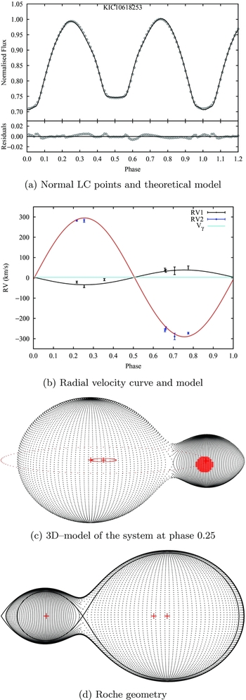
In addition to q, i, T 2, Ω1, and L 1 parameters, the semi-major axis (a) and the radial velocity of the centre of mass (V γ) were set as free parameters during the iterations. Thus, a simultaneous solution was achieved. Iterations converged to a solution, however, due to the O’Connell effect, this solution did not suffice. Therefore, a spot at a phase of around 0.25 was added on the secondary component, and the iterations were repeated to acquire the final solution. The theoretical light and radial velocity curves along with observed curves are given in Figure 6 whilst the resulting parameters are given in Table 4. According to the results of the simultaneous analysis, KIC10618253 is an A-type W UMa system which typically have low mass ratios (q < 1 as opposed to the case of q > 1 in W-type W UMa’s) meaning that the primary component is the more massive (as seen in Figure 6b) and the hotter one. Furthermore, KIC10618253 has a large fillout factor of 93% as expected for a typical A-type W UMa.

Figure 6. Results of the simultaneous analysis of the light and radial velocity curves for KIC10618253. (a) Normal LC points and theoretical model. (b) Radial velocity curve and model. (c) 3D-model of the system at phase 0.25. (d) Roche geometry.
Table 4. Results of the simultaneous light and radial velocity curve analysis of KIC10618253.

* Assumed parameter.
† r mean = (r pole r side r back)1/3.
It is crucial to emphasise here that the errors for the free parameters given in the table are not taken directly from PHOEBE, since it is frequently criticised as yielding unrealistically small error values. Therefore, we analysed each quarter’s light curve of KIC10618253 individually and then calculated the standard deviation of the 13 different values of each free parameter and gave them as estimation errors. Nevertheless, even these do not reflect the real errors since the effective temperatures of the primary components (T 1) are taken as exact values during the iterations, without reckoning with the uncertainty. Therefore, the real errors are in fact still larger than the listed ones due to the uncertainty in T 1 values.
4.3. Comparison of q sp and q ph
As seen in the results of simultaneous analysis in Table 4 and Figure 6, the spectroscopic mass ratio (q sp) of the system is 0.125. On the other hand, as seen in Figure 7 and in Table 2, the photometric mass ratio (q ph) found from grid search without any radial velocity data is 0.123, which implies that the q ph is almost perfectly coherent with the real q sp value. It should be noted that the orbital inclination (i) values are also coherent with each other (i ph = 82.4° whilst i solution = 82.654°). Although this is an expected result considering the previous theoretical works about q ph (Terrell & Wilson Reference Terrell and Wilson2005; Hambálek & Pribulla Reference Hambálek and Pribulla2013), the case of KIC10618253 itself is of course not enough for observationally proving the accuracy of the method in case of totally eclipsing systems with at least one component filling its Roche lobe. Nevertheless, we can use this example as a reliable anchor point for the sake of strengthening our claim towards the accuracy of our approximation for the rest of the systems considered here.

Figure 7. Grid search results of KIC10618253. (a) Rough search result. (b) Fine search result.
5 ABSOLUTE PARAMETERS
Since we have the radial velocity curves for only KIC10618253, in order to calculate the absolute parameters of other systems considered here, we had to use some statistically derived relations between absolute parameters (such as log P − log M, log P − log R, etc.). One of the most recent works regarding these relations is by Gazeas & Stȩpień (Reference Gazeas and Stȩpień2008). Using the W UMa sample (both A and W-type) they presented, in order to find the semi-major axis (a) value, we derived log P − log a relation, whose correlation constant is R 2 = 0.95, (Figure 8) as follows:
 $$\begin{equation}
\log a=(0.8829\pm 0.0203)\log P+(0.7900\pm 0.0082),
\end{equation}$$
$$\begin{equation}
\log a=(0.8829\pm 0.0203)\log P+(0.7900\pm 0.0082),
\end{equation}$$
where a is in R⊙ and P is in days units. Using this derived relation for the case of our anchor object KIC10618253, a = 2.971 ± 0.075 R⊙ is found, which is in good agreement with the value of 2.870 R⊙ given in Table 4. In the light of this good agreement and the goodness of the linear fit (R 2 = 0.95), we calculated the semi-major axis values of the other systems of which we do not have the radial velocity curves. Using these a(R⊙) values along with the photometric mass ratios (q ph) in the Kepler’s third law, we calculated the masses of the components individually for each system. Again, using the derived a values along with the fractional radii (r 1, 2), which resulted from the light curve analyses as r mean, we calculated the radii of the components in solar units via r 1, 2 = R 1, 2/a. The results of our calculations for the absolute parameters using equation (1) are given in Table 5.

Figure 8. The log P − log a relation derived from the sample of W UMa’s taken from Gazeas & Stȩpień (Reference Gazeas and Stȩpień2008).
Table 5. Approximately calculated absolute parameters of the systems in our sample.

a Resultant of the simultaneous analysis of light and radial velocity curves.
As we mentioned in the beginning of this section, there are other correlations that can be derived between the parameters, such as log P − M t, where M t = M 1 + M 2. We also calculated absolute parameters using this relation and compared them with each other. The derived relation is as follows:
 $$\begin{equation}
M_{\rm t}=(2.7559\pm 0.2532)\log P+(2.8925\pm 0.1022),
\end{equation}$$
$$\begin{equation}
M_{\rm t}=(2.7559\pm 0.2532)\log P+(2.8925\pm 0.1022),
\end{equation}$$
where P is in days units and M 1, 2 are in solar units. Additionally, the R 2 value of this relation is 0.52. As seen in Figure 9, the masses calculated with equations (1) and (2) do not differ significantly from each other. However, the differences may stem from the fact that uncertainty of parameters resulting from the light curve analyses are lower than the real uncertainties, thus, our error calculations may be taken as a lower limit of uncertainties.

Figure 9. Comparison of masses derived from log P − log a and log P − M relations.
According to the approximately calculated absolute parameters, positions of the systems included in our sample amongst other W UMa-type binaries are shown on the log T eff − log (L/L⊙), namely the Hertzsprung–Russell (HR) diagram, and on the log (M/M⊙) − log (R/R⊙) diagrams in Figure 10.

Figure 10. Positions of the systems we considered in this work amongst the other W UMa-type binaries. The W UMa sample was taken from Yakut & Eggleton (Reference Yakut and Eggleton2005). ZAMS and TAMS lines for various metallicity values were taken from Girardi et al. (Reference Girardi, Bressan, Bertelli and Chiosi2000). (a) HR diagrams. (b) log M − logR diagrams.
6 DISCUSSION AND CONCLUSIONS
We tried to prove the accuracy of the mass ratios determined solely from photometric data, a method which is widely used in the literature. However, this method cannot be applied to detached systems and systems having partial eclipses, as stated by Terrell & Wilson (Reference Terrell and Wilson2005), because of missing accurate radii information. As shown by Terrell & Wilson (Reference Terrell and Wilson2005) and Hambálek & Pribulla (Reference Hambálek and Pribulla2013), W UMa-type eclipsing binaries inevitably represent the most ideal case for determining photometric mass ratio, since the surface potentials of the components are equal, consequently exerting a great constraint on the possible values of the mass ratio, in addition to total eclipses which provide the most accurate radii information. Accordingly, we selected W UMa-type totally eclipsing binaries in order to compare photometric mass ratio q ph with the spectroscopic one q sp (i.e., the more precise value). As opposed to what is widely seen in the literature, we performed a grid search for both mass ratio and orbital inclination. Furthermore, in the case of KIC10618253, for which we have sufficient radial velocity data to determine the q sp, an almost perfect agreement between q sp and q ph was achieved: q sp = 0.125 ± 0.001 whereas q ph = 0.123 and i°sp = 82.654 ± 1.744 whereas i°ph = 82.4. Relying on this result, we performed grid search for the other systems in our sample.
According to the fine grid search results given in Table 2, some systems in our sample (KIC3127873, KIC4244929, KIC8539720, KIC9151972, KIC11097678, and KIC12352712) have unusually low mass ratios which are in the range 0.06 ≲ q ≲ 0.08. This might constitute an interesting result considering that there are only two cases (SX Crv-q=0.079 and AW UMa-q=0.07) in the W UMa sample provided by Gazeas & Stȩpień (Reference Gazeas and Stȩpień2008) which have such low mass ratios. Amongst these, eclipse timing variations diagram for KIC3127873, KIC8539790, and KIC12352712 exhibit a secular period decrease (Figure 11) which causes the orbit to shrink. Taking the secular period decrease and the high fillout factor of these systems into account, we can conclude that these systems will have 100% fillout factor (Rasio & Shapiro Reference Rasio and Shapiro1995) and merge into a rapidly rotating single star such as a blue straggler or FK Com type star (Şenavcı et al. Reference Şenavcı, Nelson, Özavcı, Selam and Albayrak2008; Yang & Qian Reference Yang and Qian2015). Other systems in our sample for which q ≲ 0.1 may exhibit this behaviour as well, however, their eclipse timing variations diagrams do not imply secular period decrease at least for the time being.
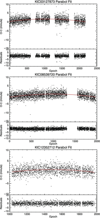
Figure 11. The eclipse timing diagrams of KIC03127873, KIC8539790 and KIC12352712.
As a result of this analysis, we have concluded that all systems considered in this work are W UMa-type eclipsing binaries of the A-subtype. This result is also supported by the HR and log M − log R diagrams given in Figure 10 in which the tendency of the systems to be amongst the A-type can be seen.
Obviously, spectroscopic observations should be made in order to justify our findings and this is our priority for the future work that we are planning to conduct. In this future work, we are planning to extend the work to W UMa-type binaries of the W-subtype and also Algol type systems having total eclipses including their radial velocity data. Thus, we can prove solidly that the photometric mass ratio method is not reliable in the case of detached binaries and partial eclipses. Furthermore, we can see whether the method is reliable in case of classical Algols (semi-detached case).
ACKNOWLEDGEMENTS
This work made use of pyke (Still & Barclay Reference Still and Barclay2012), a software package for the reduction and analysis of KEPLER data. This open source software project is developed and distributed by the NASA KEPLER Guest Observer Office. We also would like to thank the referee for his/her valuable comments.