


1 Introduction
With the introduction of the synthetic control method (SCM) (Abadie and Gardeazabal Reference Abadie and Gardeazabal2003; Abadie, Diamond, and Hainmueller Reference Abadie, Diamond and Hainmueller2010), comparative case studies using time-series cross-sectional (TSCS) data, or long panel data, are becoming increasingly popular in the social sciences. Compared with other quantitative social science research, comparative case studies have several unique features: (1) the sample includes a small number of aggregate entities; (2) a handful of units, or one, receive an intervention that is not randomly assigned; and (3) the treatment effect often takes time to present itself (Abadie Reference Abadie2020). As a result, comparative case studies face two main challenges given limited data: to “provide good predictions of the [counterfactual] trajectory of the outcome” of the treated unit(s) (Abadie, Diamond, and Hainmueller Reference Abadie, Diamond and Hainmueller2015, p. 499, henceforth, ADH Reference Abadie, Diamond and Hainmueller2015); and to make credible statistical inferences about the treatment effects.
The SCM uses a convex combination of control outcomes to predict the treated counterfactuals. Inspired by the SCM, a fast-growing literature proposes various new methods to improve the SCM’s counterfactual predictive performance and robustness, or to extend the SCM to accommodate multiple treated units. These methods can be broadly put into three categories: (1) matching or reweighting methods, such as best subset (Hsiao, Ching, and Wan Reference Hsiao, Ching and Wan2012), regularized weights (Doudchenko and Imbens Reference Doudchenko and Imbens2017), and panel matching (Imai, Kim, and Wang Reference Imai, Kim and Wang2019); (2) explicit outcome modeling approaches, such as Bayesian structural time-series models (Brodersen et al. Reference Brodersen, Gallusser, Koehler, Remy and Scott2014), latent factor models (LFMs) (e.g., Bai Reference Bai2009; Gobillon and Magnac Reference Gobillon and Magnac2016; Xu Reference Xu2017), and matrix completion methods (Athey et al. Reference Amjad, Shah and Shen2018); and (3) doubly robust methods, such as the augmented SCM (Ben-Michael, Feller, and Rothstein Reference Ben-Michael, Feller and Rothstein2020) and synthetic difference-in-differences (DiD) (Arkhangelsky et al. Reference Arkhangelsky, Athey, Hirshberg, Imbens and Wager2020).
However, both inference and prediction challenges are not fully addressed by existing methods. The SCM uses a placebo test as an inferential tool, but users cannot interpret it as a permutation test since the treatment is not randomly assigned (Hahn and Shi Reference Hahn and Shi2017). Hence, researchers cannot quantify the uncertainty of their estimates in traditional ways. Other frequentist inferential methods require a repeated sampling interpretation,Footnote 1 which is often at odds with the fixed population of units at the heart of many comparative case studies. Additionally, from a prediction perspective, researchers can use multiple sources of information in TSCS data for counterfactual prediction, including (1) temporal relationships between the known “past” and the unknown “future” of each unit, (2) cross-sectional information reflecting the similarity between units based on observed covariates, and (3) time-series relationships among units based on their outcome trajectories (Beck and Katz Reference Beck and Katz2007; Pang Reference Pang2010; Pang Reference Pang2014). While better predictive performance can translate to more precise causal estimates, existing model-based approaches make relatively rigid parametric assumptions and therefore do not take full advantage of the information in data.
The Bayesian approach is an appealing alternative to meet these challenges. First, Bayesian uncertainty measures are easy to interpret. Bayesian inference provides a solution to the inferential problem by making “probability statements conditional on observed data and an assumed model” (Gelman Reference Gelman2008, 467). Second, Bayesian multilevel modeling is a powerful tool to capture multiple sources of heterogeneity and dynamics in data (Gelman Reference Gelman2006). It can accommodate flexible functional forms and use shrinkage priors to select model features, which reduces model dependency and incorporates modeling uncertainties.
In this paper, we adopt the Bayesian causal inference framework (Rubin Reference Rubin1978; Imbens and Rubin Reference Imbens and Rubin1997; Rubin et al. Reference Rubin, Wang, Yin, Zell, O’Hagen and West2010; Ricciardi, Mattei, and Mealli Reference Ricciardi, Mattei and Mealli2020) to estimate treatment effects in comparative case studies. This framework views causal inference as a missing data problem and relies on the posterior predictive distribution of treated counterfactuals to draw inferences about the treatment effects on the treated. Missingness under this assumption falls in the category of “missing not at random” (MNAR) (Rubin Reference Rubin1976) because the assignment mechanism is allowed to be correlated to unobserved potential outcomes. The basic idea is to perform a low-rank approximation of the observed untreated outcome matrix so as to predict treated counterfactuals in the $(T\times N)$
rectangular outcome matrix. A key assumption we rely on is called latent ignorability (Ricciardi, Mattei, and Mealli Reference Ricciardi, Mattei and Mealli2020), which states that treatment assignment is ignorable conditional on exogenous covariates and an unobserved latent variable, which is learned from data.
$(T\times N)$
rectangular outcome matrix. A key assumption we rely on is called latent ignorability (Ricciardi, Mattei, and Mealli Reference Ricciardi, Mattei and Mealli2020), which states that treatment assignment is ignorable conditional on exogenous covariates and an unobserved latent variable, which is learned from data.
Conceptually, the latent ignorability assumption is an extension of the strict exogeneity assumption. Existing causal inference methods using TSCS data rely on either of the two types of assumptions for identification: strict exogeneity, which is behind the conventional two-way fixed effect approach and implies “parallel trends” in DiD designs, and sequential ignorability, which has gained popularity recently (e.g., Blackwell Reference Blackwell2013; Blackwell and Glynn Reference Blackwell and Glynn2018; Ding and Li 2018; Hazlett and Xu Reference Hazlett and Xu2018; Strezhnev Reference Strezhnev2018; Imai, Kim, and Wang Reference Imai, Kim and Wang2019). Strict exogeneity requires that treatment assignment is independent of the entire time series of potential outcomes conditional on a set of exogenous covariates and unobserved fixed effects. It rules out potential feedback effects from past outcomes on current and future treatment assignments (Imai and Kim Reference Imai and Kim2019). Its main advantage is to allow researchers to adjust for unit-specific heterogeneity and to use contemporaneous information from a fixed set of control units to predict treated counterfactuals, a key insight of the SCM. Sequential ignorability, on the other hand, allows the probability of treatment to be affected by past information including realized outcomes. In this paper, we adopt the strict exogeneity framework because it is consistent with the assumptions behind the SCM.
Specifically, we propose a dynamic multilevel latent factor model (henceforth DM-LFM) and develop an estimation strategy using Markov Chain Monte Carlo (MCMC). It incorporates a latent factor term to correct biases caused by the potential correlation between the timing of the treatment and the time-varying latent variables that can be represented by a factor structure, such as diverging trends across different units. It also allows covariate coefficients to vary by unit or over time. Because the model is parameter-rich, we use Bayesian shrinkage priors to conduct stochastic variable and factor selection, thus reducing model dependency. The MCMC algorithm we develop incorporates both model selection and parameter estimation in the same iterative sampling process.
After estimating a DM-LFM, Bayesian prediction generates the posterior distribution of each counterfactual outcome by integrating out all model parameters. We then compare the observed outcomes with the posterior distributions of their predicted counterfactuals to generate the posterior distribution of a causal effect of interest, conditional on observed data. We can use the posterior mean as the point estimate and form its uncertainty measure using the Bayesian 95% credibility interval defined by the 2.5% and 97.5% quantiles of the empirical posterior distribution. The uncertainty measure is easily interpretable: conditional on the data and assumed model, the causal effect takes values from the interval with an estimated probability of 0.95. It captures three sources of uncertainties: (1) the uncertainties from the data generating processes (DGPs), or fundamental uncertainties (King, Tomz, and Wittenberg Reference King, Tomz and Wittenberg2000); (2) the uncertainties from parameter estimation; and (3) the uncertainties from choosing the most suitable model, while existing frequentist methods, such as LFMs, only take into account the first two sources.
Several studies have used Bayesian multilevel modeling for counterfactual prediction. Some are interested in the time-series aspect of data (Belmonte, Koop, and Korobilis Reference Belmonte, Koop and Korobilis2014; de Vocht et al. Reference Vocht, Tilling, Pliakas, Angus, Egan, Brennan, Campbell and Hickman2017), in short panels (e.g., two periods) (Ricciardi, Mattei, and Mealli Reference Ricciardi, Mattei and Mealli2020), in large datasets with many treated and control units (Gutman, Intrator, and Lancaster Reference Gutman, Intrator and Lancaster2018), or in latent factor models without covariates (Samartsidis Reference Samartsidis2020). A few others have used the Bayesian approach to improve inference for comparative case studies. For example, Amjad, Shah, and Shen (Reference Athey, Bayati, Doudchenko, Imbens and Khosravi2018) adopt an empirical Bayesian approach to construct error bounds of the treatment effects, but nevertheless rely on frequentist optimization to obtain weights of the SCM. Kim, Lee, and Gupta (Reference Kim, Lee and Gupta2020) propose a fully Bayesian version of the SCM, focusing on the single treated unit case and aiming at estimating a uni-dimensional set of weights on controls.
Our method can be applied to comparative case studies with one or more treated units. Like the SCM, it requires a large number of pre-treatment periods and more control units than the treated to accurately estimate the treatment effect. Our simulation study suggests that the number of pre-treatment periods for the treated units needs to be greater than 20 for the method to achieve satisfactory frequentist properties. Compared with the SCM or LFMs, our method is most suitable when one of the following is true: (1) the uncertainty measures bear important policy or theoretical implications; (2) researchers suspect the latent factor structure is complex, the number of factors is large, or some of the factors are relatively weak; (3) many potential pre-treatment covariates are available and their relationships with the outcome variable may vary across units or over time; or (4) researchers have limited knowledge of how to select covariates for counterfactual prediction. Compared to its frequentist alternatives, this Bayesian method is computationally intense. We therefore develop an R package bpCausal, whose core functions are written in C++, for researchers to efficiently implement this method.
2 Bayesian Causal Inference: Posterior Predictive Distributions
We start by introducing the basic setting and fixing notations. We then define causal quantities of interest and develop posterior predictive distributions of counterfactuals based on several key assumptions. When doing so, we will use two empirical examples. The first one is on German reunification from ADH (Reference Abadie, Diamond and Hainmueller2015). It is appealing to illustrate our method for several reasons. First, only one unit (West Germany) in the dataset was treated, and the treatment—a historical event—took place only once. Second, the control group consists of 16 Organization for Economic Co-operation and Development (OECD) member countries, and no single country in this group or their simple average can serve as an appropriate counterfactual for West Germany. Furthermore, the impact of reunification may emerge gradually over time. The second example concerns the effect of election day registration (EDR) on voter turnout in the United States. Xu (Reference Xu2017) uses this example to demonstrate a frequentist LFM (a.k.a. the generalized synthetic control method, or Gsynth). Compared to the first example, it represents a more general setting of comparative case studies in which there are multiple treated units and the treatment starts at different points in time.
2.1 Setup and Estimands
We denote $i=1, 2,\ldots , N$
and
$i=1, 2,\ldots , N$
and $t=1, 2,\ldots , T$
as the unit and time for which and when the outcome of interest is observed. Although our method can accommodate imbalanced panels, we assume a balanced panel instead for notational convenience. We consider a binary treatment
$t=1, 2,\ldots , T$
as the unit and time for which and when the outcome of interest is observed. Although our method can accommodate imbalanced panels, we assume a balanced panel instead for notational convenience. We consider a binary treatment $w_{it}$
that, once it takes a value of 1, cannot reverse back to 0 (staggered adoption). Following Athey and Imbens (Reference Athey and Imbens2018), we define the timing of adoption for each unit i as a random variable
$w_{it}$
that, once it takes a value of 1, cannot reverse back to 0 (staggered adoption). Following Athey and Imbens (Reference Athey and Imbens2018), we define the timing of adoption for each unit i as a random variable $a_{i}$
that takes its values in
$a_{i}$
that takes its values in $\mathbb {A}= \{1,2,\ldots , T, c\}$
, in which
$\mathbb {A}= \{1,2,\ldots , T, c\}$
, in which $a_{i} = c> T$
means that unit i falls in the residual category and does not get treated in the observed time window. We call unit i a treated unit if it adopts the treatment at any of the observed time periods (
$a_{i} = c> T$
means that unit i falls in the residual category and does not get treated in the observed time window. We call unit i a treated unit if it adopts the treatment at any of the observed time periods ( $a_{i}=1, 2,\ldots , T$
); we call it a control unit if it never adopts the treatment by period
$a_{i}=1, 2,\ldots , T$
); we call it a control unit if it never adopts the treatment by period $T\ (a_{i} = c$
). The number of pre-treatment periods for a treated unit is
$T\ (a_{i} = c$
). The number of pre-treatment periods for a treated unit is $T_{0,i} = a_{i} -1$
. Suppose there are
$T_{0,i} = a_{i} -1$
. Suppose there are $N_{co}$
control units and
$N_{co}$
control units and $N_{tr}$
treated units;
$N_{tr}$
treated units; $N_{co} + N_{tr} = N$
. In comparative case studies,
$N_{co} + N_{tr} = N$
. In comparative case studies, $N_{tr}=1$
or a small integer.
$N_{tr}=1$
or a small integer.
For instance, in the German reunification example, $i=1,\ldots , 17$
,
$i=1,\ldots , 17$
, $T = 1, 2,\ldots , 44$
. West Germany’s
$T = 1, 2,\ldots , 44$
. West Germany’s $a_{i}$
is
$a_{i}$
is $31$
(the calendar year 1990); and
$31$
(the calendar year 1990); and $a_{i}>44$
for the other 16 OECD countries serving as controls. The EDR example uses the data of 47 states (
$a_{i}>44$
for the other 16 OECD countries serving as controls. The EDR example uses the data of 47 states ( $i=1,\ldots , 47$
) in 24 presidential election years from 1920 to 2012 (
$i=1,\ldots , 47$
) in 24 presidential election years from 1920 to 2012 ( $t=1,\ldots ,24)$
. Among the 47 states, 9 states adopted EDR before 2012, whose
$t=1,\ldots ,24)$
. Among the 47 states, 9 states adopted EDR before 2012, whose $a_{i} \in \{15, 20, 23, 24\}$
; they are considered the treated units. The other 38 states did not adopt EDR by 2012 (
$a_{i} \in \{15, 20, 23, 24\}$
; they are considered the treated units. The other 38 states did not adopt EDR by 2012 ( $a_{i}>24$
) and are considered the control units.
$a_{i}>24$
) and are considered the control units.
Denote $\textbf{w}_{i} = (w_{i1},\ldots , w_{iT})^{\prime }$
as the treatment assignment vector for unit i. Staggered adoption implies that the adoption time
$\textbf{w}_{i} = (w_{i1},\ldots , w_{iT})^{\prime }$
as the treatment assignment vector for unit i. Staggered adoption implies that the adoption time $a_{i}$
uniquely determines vector
$a_{i}$
uniquely determines vector $\textbf{w}_{i}$
:
$\textbf{w}_{i}$
: $\textbf{w}_{i}(a_{i})$
, in which
$\textbf{w}_{i}(a_{i})$
, in which ${w_{it}=0}$
if
${w_{it}=0}$
if $t<a_{i}$
and
$t<a_{i}$
and ${w_{it}=1}$
if
${w_{it}=1}$
if $t \geqslant a_{i}$
, for
$t \geqslant a_{i}$
, for $t=1, 2,\ldots , T$
. We further define an
$t=1, 2,\ldots , T$
. We further define an $(N\times T)$
treatment assignment matrix,
$(N\times T)$
treatment assignment matrix, $ \textbf {W} =\{\textbf{w}_{1},\ldots , \textbf{w}_{N} \}$
; similarly,
$ \textbf {W} =\{\textbf{w}_{1},\ldots , \textbf{w}_{N} \}$
; similarly, $\textbf {W}$
is fully determined by
$\textbf {W}$
is fully determined by $\mathcal {A}=\{a_{1},\ldots , a_{i},\ldots , a_{N} \}$
, the adoption time vector. Following Athey and Imbens (Reference Athey and Imbens2018), we make the following two assumptions to rule out cross-sectional spillover and the anticipation effect.
$\mathcal {A}=\{a_{1},\ldots , a_{i},\ldots , a_{N} \}$
, the adoption time vector. Following Athey and Imbens (Reference Athey and Imbens2018), we make the following two assumptions to rule out cross-sectional spillover and the anticipation effect.
Assumption 1 (Cross-sectional stable unit treatment value assumption (SUTVA))
Potential outcomes of unit i are only functions of the treatment status of unit i: $\textbf {y}_{it} (\textbf{W}) = \textbf {y}_{it} (\textbf{w}_{i}), \forall i, \ t$
.
$\textbf {y}_{it} (\textbf{W}) = \textbf {y}_{it} (\textbf{w}_{i}), \forall i, \ t$
.
This assumption rules out cross-sectional spillover effects and significantly reduces the number of potential outcome trajectories. For each unit i, because now there are only $(T+1)$
possibilities for
$(T+1)$
possibilities for $\textbf{w}_{i}$
, there are
$\textbf{w}_{i}$
, there are $(T+1)$
potential outcome trajectories, denoted by
$(T+1)$
potential outcome trajectories, denoted by $y_{it}(\textbf{w}_{i}), \ t = 1, 2,\ldots , T$
. In the German reunification example, this assumption rules out the possibility that German reunification affects economic growth in the other 16 countries, which may, in fact, be a strong assumption. In the EDR example, this assumption implies that the adoption of EDR laws in State B does not affect State A’s turnout with or without EDR laws. Because
$y_{it}(\textbf{w}_{i}), \ t = 1, 2,\ldots , T$
. In the German reunification example, this assumption rules out the possibility that German reunification affects economic growth in the other 16 countries, which may, in fact, be a strong assumption. In the EDR example, this assumption implies that the adoption of EDR laws in State B does not affect State A’s turnout with or without EDR laws. Because $\textbf{w}_{i}$
is fully determined by
$\textbf{w}_{i}$
is fully determined by $a_{i}$
, we simply write
$a_{i}$
, we simply write $y_{it}(\textbf{w}_{i}(a_{i}))$
as
$y_{it}(\textbf{w}_{i}(a_{i}))$
as $y_{it}(a_{i})$
.
$y_{it}(a_{i})$
.
Assumption 2 (No anticipation)
For all unit i, for all time periods before adoption $t < a_{i}$
:
$t < a_{i}$
:
 $$ \begin{align*} y_{it}(a_{i}) = y_{it}(c), \mbox{ for } t < a_{i}, \forall i \end{align*} $$
in which $y_{it}(c)$
is the potential outcome under the “pure control” condition, that is, the treatment vector
$y_{it}(c)$
is the potential outcome under the “pure control” condition, that is, the treatment vector $\textbf{w}_{i}$
includes all zeros. This assumption says that the current untreated potential outcome does not depend on whether the unit gets the treatment in the future. The assumption is violated when anticipating that a unit will adopt the treatment in the future affects its outcome today. For example, if people anticipated German reunification to take place in 1990 and West Germany’s economy adjusted to that expectation before 1990, the assumption would be violated.
$\textbf{w}_{i}$
includes all zeros. This assumption says that the current untreated potential outcome does not depend on whether the unit gets the treatment in the future. The assumption is violated when anticipating that a unit will adopt the treatment in the future affects its outcome today. For example, if people anticipated German reunification to take place in 1990 and West Germany’s economy adjusted to that expectation before 1990, the assumption would be violated.
Estimands
Under Assumptions 1 and 2, for treated unit i whose adoption time $a_{i} \leqslant T$
, we define its treatment effect at
$a_{i} \leqslant T$
, we define its treatment effect at $t \geqslant a_{i}$
as
$t \geqslant a_{i}$
as
 $$ \begin{align*} \delta_{it} = y_{it}(a_{i}) - y_{it}(c), \mbox{ for } a_{i}\leqslant t \leqslant T. \end{align*} $$
In other words, we focus on the difference between the observed post-treatment outcome of treated unit i and the counterfactual outcome of the same unit that had never received the treatment by period $T\!$
. In the German reunification example, the causal effect of interest is the difference between the observed gross domestic product (GDP) per capita of West Germany in reunified Germany since 1990 and that of the counterfactual West Germany had it remained separated from East Germany.
$T\!$
. In the German reunification example, the causal effect of interest is the difference between the observed gross domestic product (GDP) per capita of West Germany in reunified Germany since 1990 and that of the counterfactual West Germany had it remained separated from East Germany.
Because $y_{it}(a_{i})$
of treated unit i is fully observed for
$y_{it}(a_{i})$
of treated unit i is fully observed for $t\geqslant a_{i}$
, the Bayesian framework regards it as data. The counterfactual outcome
$t\geqslant a_{i}$
, the Bayesian framework regards it as data. The counterfactual outcome $y_{it}(c)$
of treated unit i for
$y_{it}(c)$
of treated unit i for $t\geqslant a_{i}$
, on the other hand, is an unknown quantity; we regard it as a random variable. We also define the sample average treatment effect on the treated (ATT) for units that have been under the treatment for a duration of p periods:
$t\geqslant a_{i}$
, on the other hand, is an unknown quantity; we regard it as a random variable. We also define the sample average treatment effect on the treated (ATT) for units that have been under the treatment for a duration of p periods: $\delta _{p} = \frac {1}{N_{tr,p}} \sum _{i: T - p + 1 \leqslant a_{i}\leqslant T} \delta _{i, a_{i}+p-1}$
, where
$\delta _{p} = \frac {1}{N_{tr,p}} \sum _{i: T - p + 1 \leqslant a_{i}\leqslant T} \delta _{i, a_{i}+p-1}$
, where $N_{tr,p}$
is the number of treated units that have been treated for p periods in the sample.
$N_{tr,p}$
is the number of treated units that have been treated for p periods in the sample.
Given that $y_{it}(a_{i})$
is observed in the post-treatment period, estimating
$y_{it}(a_{i})$
is observed in the post-treatment period, estimating $\delta _{it}$
is equivalent to constructing the counterfactual outcome
$\delta _{it}$
is equivalent to constructing the counterfactual outcome $y_{it}(c)$
. Under Assumptions 1 and 2, we can denote
$y_{it}(c)$
. Under Assumptions 1 and 2, we can denote $\textbf {Y}(\textbf {0})$
, a
$\textbf {Y}(\textbf {0})$
, a $(N\times T)$
matrix, as the potential outcome matrix under
$(N\times T)$
matrix, as the potential outcome matrix under $\textbf{W}=\textbf {0}$
(i.e.,
$\textbf{W}=\textbf {0}$
(i.e., $a_{i}=c, \forall i$
). Given any realization of
$a_{i}=c, \forall i$
). Given any realization of $\textbf{W}$
, we can partition the indices for
$\textbf{W}$
, we can partition the indices for $\textbf {Y}(\textbf {0})$
into two sets:
$\textbf {Y}(\textbf {0})$
into two sets: $S_{0} \equiv \{(it)| w_{it} =0\}$
, with which
$S_{0} \equiv \{(it)| w_{it} =0\}$
, with which $y_{it}(c)$
is observed; and
$y_{it}(c)$
is observed; and $S_{1} \equiv \{(it)| w_{it} =1\}$
, with which
$S_{1} \equiv \{(it)| w_{it} =1\}$
, with which $y_{it}(c)$
is missing. Additionally,
$y_{it}(c)$
is missing. Additionally, $S=S_{0} \cup S_{1}$
. We denote the observed and missing parts of
$S=S_{0} \cup S_{1}$
. We denote the observed and missing parts of $\textbf {Y}(\textbf {0})$
as
$\textbf {Y}(\textbf {0})$
as $\textbf {Y}(\textbf {0})^{obs}$
and
$\textbf {Y}(\textbf {0})^{obs}$
and $\textbf {Y}(\textbf {0})^{mis}$
, respectively, and
$\textbf {Y}(\textbf {0})^{mis}$
, respectively, and $\textbf {Y}_{i}(\textbf {0})^{obs}$
and
$\textbf {Y}_{i}(\textbf {0})^{obs}$
and $\textbf {Y}_{i}(\textbf {0})^{mis}$
as the row vectors in
$\textbf {Y}_{i}(\textbf {0})^{mis}$
as the row vectors in $\textbf {Y}(\textbf {0})^{obs}$
and
$\textbf {Y}(\textbf {0})^{obs}$
and $\textbf {Y}(\textbf {0})^{mis}$
corresponding to unit i, respectively.
$\textbf {Y}(\textbf {0})^{mis}$
corresponding to unit i, respectively. $\textbf {X}_{it}$
is a
$\textbf {X}_{it}$
is a $(p_{1} \times 1)$
vector of exogenous covariates.
$(p_{1} \times 1)$
vector of exogenous covariates. $\textbf {X}_{i} = (\textbf {X}_{i1}, \ldots , \textbf {X}_{iT})^{\prime }$
is a
$\textbf {X}_{i} = (\textbf {X}_{i1}, \ldots , \textbf {X}_{iT})^{\prime }$
is a $(T\times p_{1})$
covariate matrix, and we define
$(T\times p_{1})$
covariate matrix, and we define $\textbf {X} = \{\textbf {X}_{1}, \textbf {X}_{2}, \cdots , \textbf {X}_{N}\}$
.
$\textbf {X} = \{\textbf {X}_{1}, \textbf {X}_{2}, \cdots , \textbf {X}_{N}\}$
.
2.2 The Assignment Mechanism
Rubin et al. (Reference Rubin, Wang, Yin, Zell, O’Hagen and West2010) lay down the fundamentals of Bayesian causal inference, which views “causal inference entirely as a missing data problem” (p. 685). In general, using the observed outcomes and covariates, as well as the assignment mechanism, we can stochastically impute counterfactuals from their posterior predictive distribution $\Pr (\textbf {Y}(\textbf{W})^{mis} |\textbf {X}, \textbf {Y}(\textbf{W})^{obs}, \textbf{W})$
. Since in this research the main causal quantity of interest is the (average) treatment effect on the treated, our primary goal is to predict counterfactuals
$\Pr (\textbf {Y}(\textbf{W})^{mis} |\textbf {X}, \textbf {Y}(\textbf{W})^{obs}, \textbf{W})$
. Since in this research the main causal quantity of interest is the (average) treatment effect on the treated, our primary goal is to predict counterfactuals $\textbf {Y}(\textbf {0})^{mis}$
, the untreated outcomes of the treated units. Because staggered adoption implies that
$\textbf {Y}(\textbf {0})^{mis}$
, the untreated outcomes of the treated units. Because staggered adoption implies that $\textbf{W}$
is fully determined by
$\textbf{W}$
is fully determined by $\mathcal {A}$
, the adoption time vector, we write the posterior predictive distribution of
$\mathcal {A}$
, the adoption time vector, we write the posterior predictive distribution of $\textbf {Y}(\textbf {0})^{mis}$
as
$\textbf {Y}(\textbf {0})^{mis}$
as
 $$ \begin{align} \Pr (\textbf{Y}(\textbf{0})^{mis}|\textbf{X}, \textbf{Y}(\textbf{0})^{obs}, \mathcal{A}) =& \frac{\Pr(\textbf{X}, \textbf{Y}(\textbf{0})^{mis}, \textbf{Y}(\textbf{0})^{obs})\Pr(\mathcal{A}|\textbf{X}, \textbf{Y}(\textbf{0})^{mis}, \textbf{Y}(\textbf{0})^{obs})}{\Pr(\textbf{X}, \textbf{Y}(\textbf{0})^{obs}, \mathcal{A})} \nonumber\\ \propto& \Pr(\textbf{X}, \textbf{Y}(\textbf{0})^{mis}, \textbf{Y}(\textbf{0})^{obs}) \Pr(\mathcal{A}|\textbf{X}, \textbf{Y}(\textbf{0})^{mis}, \textbf{Y}(\textbf{0})^{obs})\nonumber\\ \propto & \Pr(\textbf{X}, \textbf{Y}(\textbf{0})) \Pr(\mathcal{A}|\textbf{X}, \textbf{Y}(\textbf{0})). \end{align} $$
The Bayes rule gives the equality in Equation (1), and we obtain the proportionality by dropping the denominator as a normalizing constant since it contains no missing data. Hence, two component probabilities, the underlying “science” $\Pr (\textbf {X}, \textbf {Y}(\textbf {0}))$
and the treatment assignment mechanism
$\Pr (\textbf {X}, \textbf {Y}(\textbf {0}))$
and the treatment assignment mechanism $\Pr (\mathcal {A}|\textbf {X}, \textbf {Y}(\textbf {0}))$
, help predict the counterfactuals.
$\Pr (\mathcal {A}|\textbf {X}, \textbf {Y}(\textbf {0}))$
, help predict the counterfactuals.
Assumption 3 (Individualistic assignment and positivity) $\Pr (\mathcal {A}|\textbf{X}, \textbf{Y}(\textbf{0}))= \prod _{i=1}^{n} \Pr (a_{i}|\textbf{X}_{i}, \textbf{Y}_{i}(\textbf{0}))$
and
$\Pr (\mathcal {A}|\textbf{X}, \textbf{Y}(\textbf{0}))= \prod _{i=1}^{n} \Pr (a_{i}|\textbf{X}_{i}, \textbf{Y}_{i}(\textbf{0}))$
and $ 0 < \Pr (a_{i}|\textbf{X}_{i}, \textbf{Y}_{i}(\textbf{0})) < 1$
for all unit i.
$ 0 < \Pr (a_{i}|\textbf{X}_{i}, \textbf{Y}_{i}(\textbf{0})) < 1$
for all unit i.
We assume that the treatment assignment is “individualistic” (Imbens and Rubin Reference Imbens and Rubin2015, 31), that is, the adoption time of unit i does not depend on the covariates or potential outcomes of other units or their time of adoption, given $\textbf{X}_{i}$
and
$\textbf{X}_{i}$
and $\textbf{Y}_{i}(\textbf {0})$
. We also require that each i has some nonzero chances of getting treated. The first part of this assumption is violated if policy diffusion takes place—for example, State A adopts EDR following State B’s policy shift—and such an emulation effect cannot be captured by a unit’s pre-treatment covariates and untreated potential outcomes. The positivity assumption means that all units in the sample have some probability of getting treated, thus justifying using control information to predict treated counterfactuals.
$\textbf{Y}_{i}(\textbf {0})$
. We also require that each i has some nonzero chances of getting treated. The first part of this assumption is violated if policy diffusion takes place—for example, State A adopts EDR following State B’s policy shift—and such an emulation effect cannot be captured by a unit’s pre-treatment covariates and untreated potential outcomes. The positivity assumption means that all units in the sample have some probability of getting treated, thus justifying using control information to predict treated counterfactuals.
The fact that $\Pr (a_{i}|\textbf{X}_{i}, \textbf{Y}_{i}(\textbf {0})) =\Pr (a_{i}|\textbf{X}_{i}, \textbf{Y}_{i}(\textbf {0})^{obs}, \textbf{Y}_{i}(\textbf {0})^{mis})$
implies that the treatment assignment mechanism may be correlated with
$\Pr (a_{i}|\textbf{X}_{i}, \textbf{Y}_{i}(\textbf {0})) =\Pr (a_{i}|\textbf{X}_{i}, \textbf{Y}_{i}(\textbf {0})^{obs}, \textbf{Y}_{i}(\textbf {0})^{mis})$
implies that the treatment assignment mechanism may be correlated with $\textbf{Y}_{i}(\textbf {0})^{mis}$
. To rule out potential confounding, one possibility is to impose further restrictions and make an ignorability assignment assumption
$\textbf{Y}_{i}(\textbf {0})^{mis}$
. To rule out potential confounding, one possibility is to impose further restrictions and make an ignorability assignment assumption $\Pr (a_{i}|\textbf{X}_{i}, \textbf{Y}_{i}(\textbf {0})^{obs})$
(Rubin Reference Rubin1978). However, in the more general setting of MNAR, this restriction is unlikely to be true. For instance, the timing of a state’s adopting an EDR law could be driven by legislators’ concern about future voter turnout in the absence of such laws. Therefore, we rely on the latent ignorability assumption to break the link between treatment assignment and control outcomes.
$\Pr (a_{i}|\textbf{X}_{i}, \textbf{Y}_{i}(\textbf {0})^{obs})$
(Rubin Reference Rubin1978). However, in the more general setting of MNAR, this restriction is unlikely to be true. For instance, the timing of a state’s adopting an EDR law could be driven by legislators’ concern about future voter turnout in the absence of such laws. Therefore, we rely on the latent ignorability assumption to break the link between treatment assignment and control outcomes.
Assumption 4 (Latent ignorability)
Conditional on the observed pre-treatment covariates $\textbf{X}_{i}$
and a vector of latent variables
$\textbf{X}_{i}$
and a vector of latent variables $\textbf{U}_{i} = (u_{i1}, u_{i2}, \cdots , u_{iT})$
, the assignment mechanism is free from dependence on any missing or observed untreated outcomes for each unit i, that is,
$\textbf{U}_{i} = (u_{i1}, u_{i2}, \cdots , u_{iT})$
, the assignment mechanism is free from dependence on any missing or observed untreated outcomes for each unit i, that is,
 $$ \begin{align} \Pr(a_{i}|\textbf{X}_{i}, \textbf{Y}_{i}(\textbf{0}), \textbf{U}_{i}) = \Pr(a_{i}|\textbf{X}_{i}, \textbf{Y}_{i}(\textbf{0})^{mis}, \textbf{Y}_{i}(\textbf{0})^{obs}, \textbf{U}_{i}) = \Pr(a_{i}|\textbf{X}_{i}, \textbf{U}_{i}). \end{align} $$
Note that $\textbf{X}_{i}$
can include both time-varying and time-invariant pre-treatment covariates.
$\textbf{X}_{i}$
can include both time-varying and time-invariant pre-treatment covariates. $\textbf {U}_{i}$
captures both unit-level heterogeneity, such as unit fixed effects, and unit-specific time trends (e.g.,
$\textbf {U}_{i}$
captures both unit-level heterogeneity, such as unit fixed effects, and unit-specific time trends (e.g., $u_{it} = \gamma _{i} \cdot g(t)$
, in which
$u_{it} = \gamma _{i} \cdot g(t)$
, in which $g(\cdot )$
is a function of time). We expect
$g(\cdot )$
is a function of time). We expect $\textbf {U}_{i}$
to be correlated with
$\textbf {U}_{i}$
to be correlated with $\textbf{Y}_{i}(\textbf {0})$
; in fact, we will extract it from
$\textbf{Y}_{i}(\textbf {0})$
; in fact, we will extract it from $\textbf{Y}_{i}(\textbf {0})^{obs}$
. Therefore, once we condition on
$\textbf{Y}_{i}(\textbf {0})^{obs}$
. Therefore, once we condition on $\textbf{X}_{i}$
and
$\textbf{X}_{i}$
and $\textbf {U}_{i}$
, the entire time series of
$\textbf {U}_{i}$
, the entire time series of $\textbf{Y}_{i}(\textbf {0})$
is assumed to be independent of
$\textbf{Y}_{i}(\textbf {0})$
is assumed to be independent of $a_{i}$
. Thus, we can understand Assumption 4 as an extension of the strict exogeneity assumption often assumed in fixed effects models. Like strict exogeneity, it rules out dynamic feedback from the past outcomes on current and future treatment assignments, conditional on
$a_{i}$
. Thus, we can understand Assumption 4 as an extension of the strict exogeneity assumption often assumed in fixed effects models. Like strict exogeneity, it rules out dynamic feedback from the past outcomes on current and future treatment assignments, conditional on $\textbf {U}_{i}$
.
$\textbf {U}_{i}$
.
The latent ignorability assumption is key to our approach. It is easy to see that the “parallel trends” assumption is implied by this assumption when $\textbf {U}_{i}$
is a unit-specific constant
$\textbf {U}_{i}$
is a unit-specific constant $u_{i1} = u_{i2} = \cdots = u_{iT} = u_{i}$
. What does this assumption mean substantively? In the EDR example, suppose there is an unmeasured downward trend in voter turnout in all states since the 1970s, driven by unknown socioeconomic forces. Its impact may be different across states due to differences in geography, demography, party organizations, ideological orientation, and so on. At the same time, the adoption of EDR in a state is correlated with how much such a trend would affect the state’s turnout in the absence of any policy changes. In this case, the “parallel time trends” assumption is invalid because
$u_{i1} = u_{i2} = \cdots = u_{iT} = u_{i}$
. What does this assumption mean substantively? In the EDR example, suppose there is an unmeasured downward trend in voter turnout in all states since the 1970s, driven by unknown socioeconomic forces. Its impact may be different across states due to differences in geography, demography, party organizations, ideological orientation, and so on. At the same time, the adoption of EDR in a state is correlated with how much such a trend would affect the state’s turnout in the absence of any policy changes. In this case, the “parallel time trends” assumption is invalid because $u_{it}$
is a time-varying confounder; however, we can correct for the biases if we can estimate, then condition on, the state-specific impact of this common trend. Hence, we further make a feasibility assumption.
$u_{it}$
is a time-varying confounder; however, we can correct for the biases if we can estimate, then condition on, the state-specific impact of this common trend. Hence, we further make a feasibility assumption.
Assumption 5 (Feasible data extraction)
Assume that, for each unit i, there exists an unobserved covariate vector $\textbf{U}_{i}$
for each unit i, such that the stacked
$\textbf{U}_{i}$
for each unit i, such that the stacked $(N\times T)$
matrix
$(N\times T)$
matrix $\textbf{U} = (\textbf{U}_{1},\ldots , \textbf{U}_{N})$
can be approximated by two lower-rank matrices (
$\textbf{U} = (\textbf{U}_{1},\ldots , \textbf{U}_{N})$
can be approximated by two lower-rank matrices ( $r\ll \min \{N, T\}$
), that is,
$r\ll \min \{N, T\}$
), that is, $\textbf{U} = \boldsymbol {\Gamma }^{\prime }\textbf {F}$
in which
$\textbf{U} = \boldsymbol {\Gamma }^{\prime }\textbf {F}$
in which $\textbf {F}=(\textbf {f}_{1},\ldots , \textbf {f}_{T})$
is a
$\textbf {F}=(\textbf {f}_{1},\ldots , \textbf {f}_{T})$
is a $(r\times T)$
matrix of factors and
$(r\times T)$
matrix of factors and $\boldsymbol {\Gamma }=(\boldsymbol {\gamma }_{1},\ldots , \boldsymbol {\gamma }_{N})$
is a
$\boldsymbol {\Gamma }=(\boldsymbol {\gamma }_{1},\ldots , \boldsymbol {\gamma }_{N})$
is a $(r\times N)$
matrix of the factor loadings.
$(r\times N)$
matrix of the factor loadings.
This assumption is explicitly or implicitly made with the factor-augmented approach in the existing literature (Xu Reference Xu2017; Athey et al. Reference Athey, Bayati, Doudchenko, Imbens and Khosravi2018; Bai and Ng Reference Bai and Ng2020). It says that we can decompose the unit-specific time trends into multiple common trends with heterogeneous impacts. Assumption 5 is violated when $\textbf{U}_{1},\ldots , \textbf{U}_{n}$
have no common components; for example, when unit-specific time trends are idiosyncratic.
$\textbf{U}_{1},\ldots , \textbf{U}_{n}$
have no common components; for example, when unit-specific time trends are idiosyncratic.
2.3 Posterior Predictive Inference
Under Assumption 4, we temporarily consider $\textbf{U}$
as part of the covariates and write
$\textbf{U}$
as part of the covariates and write $\textbf{X}$
and
$\textbf{X}$
and $\textbf{U}$
together as
$\textbf{U}$
together as $\textbf{X}^{\prime }$
. Then we have the posterior predictive distribution of
$\textbf{X}^{\prime }$
. Then we have the posterior predictive distribution of $\textbf {Y}(\textbf {0})^{mis}$
as
$\textbf {Y}(\textbf {0})^{mis}$
as
 $$ \begin{align} \Pr (\textbf{Y}(\textbf{0})^{mis}|\textbf{X}^{\prime}, \textbf{Y}(\textbf{0})^{obs}, \mathcal{A}) &\propto \Pr(\textbf{X}^{\prime}, \textbf{Y}(\textbf{0})^{mis}, \textbf{Y}(\textbf{0})^{obs}) \Pr(\mathcal{A}|\textbf{X}^{\prime}, \textbf{Y}(\textbf{0})^{mis}, \textbf{Y}(\textbf{0})^{obs})\nonumber\\ &\propto \Pr (\textbf{X}^{\prime}, \textbf{Y}(\textbf{0})^{mis}, \textbf{Y}(\textbf{0})^{obs}) \Pr(\mathcal{A}|\textbf{X}^{\prime}) \nonumber\\ &\propto \Pr(\textbf{X}^{\prime}, \textbf{Y}(\textbf{0})). \end{align} $$
The first line is simply to re-write Equation (1) by replacing $\textbf{X}$
with
$\textbf{X}$
with $\textbf{X}^{\prime }$
; we reach the second step using the latent ignorability assumption; the last step drops the treatment assignment mechanism
$\textbf{X}^{\prime }$
; we reach the second step using the latent ignorability assumption; the last step drops the treatment assignment mechanism $\Pr (\mathcal {A}|\textbf{X}^{\prime })$
as a normalizing constant since it does not contain
$\Pr (\mathcal {A}|\textbf{X}^{\prime })$
as a normalizing constant since it does not contain $\textbf {Y}(\textbf {0})^{mis}$
.
$\textbf {Y}(\textbf {0})^{mis}$
.
Equation (3) says that the latent ignorability assumption makes the treatment assignment mechanism ignorable in counterfactual prediction; as a result, we can ignore it as long as we condition on $\textbf{X}^{\prime }$
. In other words, under these assumptions, the task of developing the posterior predictive distributions of counterfactuals is reduced to model
$\textbf{X}^{\prime }$
. In other words, under these assumptions, the task of developing the posterior predictive distributions of counterfactuals is reduced to model $\Pr (\textbf{X}^{\prime }, \textbf {Y}(\textbf {0})) $
. We need this trick because in comparative case studies, the number of treated units is small; as a result, we lack sufficient variation of the timing of adoption in data to model
$\Pr (\textbf{X}^{\prime }, \textbf {Y}(\textbf {0})) $
. We need this trick because in comparative case studies, the number of treated units is small; as a result, we lack sufficient variation of the timing of adoption in data to model $\Pr (\mathcal {A}|\textbf{X}^{\prime })$
. To model the underlying “science,” we further make the assumption of exchangeability:
$\Pr (\mathcal {A}|\textbf{X}^{\prime })$
. To model the underlying “science,” we further make the assumption of exchangeability:
Assumption 6 (Exchangeability)
When $\textbf{U}$
is known,
$\textbf{U}$
is known, $\{(\textbf{X}_{it}^{\prime }, y_{it}(c))\}_{i = 1,\dots ,N; t = 1,\dots , T}$
is an exchangeable sequence of random variables; that is, the joint distribution of
$\{(\textbf{X}_{it}^{\prime }, y_{it}(c))\}_{i = 1,\dots ,N; t = 1,\dots , T}$
is an exchangeable sequence of random variables; that is, the joint distribution of $\{(\textbf{X}_{it}^{\prime }, y_{it}(c))\}$
is invariant to permutations in the index
$\{(\textbf{X}_{it}^{\prime }, y_{it}(c))\}$
is invariant to permutations in the index $it$
.
$it$
.
By de Finetti’s theorem (de Finetti Reference de Finetti, Kyburg and Smokler1963), $\{(\textbf{X}_{it}^{\prime }, y_{it}(c))\}$
can be written as i.i.d, given some parameters and their prior distributions. Note that
$\{(\textbf{X}_{it}^{\prime }, y_{it}(c))\}$
can be written as i.i.d, given some parameters and their prior distributions. Note that $\Pr (\textbf{X}^{\prime }, \textbf {Y}(\textbf {0}))$
is equivalent to
$\Pr (\textbf{X}^{\prime }, \textbf {Y}(\textbf {0}))$
is equivalent to $\Pr (\{(\textbf{X}_{it}^{\prime }, y_{it}(c))\})$
, and we now can write the posterior predictive distribution of
$\Pr (\{(\textbf{X}_{it}^{\prime }, y_{it}(c))\})$
, and we now can write the posterior predictive distribution of $\textbf {Y}(\textbf {0})^{mis}$
in Equation (3) as
$\textbf {Y}(\textbf {0})^{mis}$
in Equation (3) as
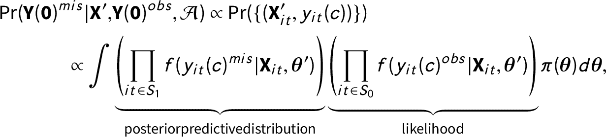 $$ \begin{align} \Pr (\textbf{Y}(\textbf{0})^{mis}|\textbf{X}^{\prime}, &\textbf{Y}(\textbf{0})^{obs}, \mathcal{A}) \propto \Pr(\{(\textbf{X}_{it}^{\prime}, y_{it}(c)) \}) \nonumber \\ \propto \int &\underbrace{\left(\prod_{it \in S_{1}} f(y_{it}(c)^{mis}|\textbf{X}_{it}, \boldsymbol{\theta}^{\prime}) \right)}_{{{\rm posterior predictive distribution}}} \underbrace{\left(\prod_{it \in S_{0}} f(y_{it}(c)^{obs}|\textbf{X}_{it}, \boldsymbol{\theta}^{\prime})\right)}_{{{\rm likelihood}}}\pi(\boldsymbol{\theta}) d \boldsymbol{\theta}, \end{align} $$
where $\boldsymbol {\theta }$
are the parameters that govern the DGP of
$\boldsymbol {\theta }$
are the parameters that govern the DGP of $y_{it}(c)$
given
$y_{it}(c)$
given $\textbf{X}^{\prime }_{it}$
, and
$\textbf{X}^{\prime }_{it}$
, and $\boldsymbol {\theta }^{\prime }=(\boldsymbol {\theta }, \textbf{U})$
when we regard the latent covariates
$\boldsymbol {\theta }^{\prime }=(\boldsymbol {\theta }, \textbf{U})$
when we regard the latent covariates $\textbf{U}$
as parameters. Note that in Equation (4), the likelihood is based on observed outcomes while the posterior predictive distribution is for predicting the missing potential outcomes. The second proportionality is reached by de Finetti’s theorem and under the assumption that the set of parameters that govern the DGP of the covariates
$\textbf{U}$
as parameters. Note that in Equation (4), the likelihood is based on observed outcomes while the posterior predictive distribution is for predicting the missing potential outcomes. The second proportionality is reached by de Finetti’s theorem and under the assumption that the set of parameters that govern the DGP of the covariates $\textbf{X}$
are independent of
$\textbf{X}$
are independent of $\boldsymbol {\theta }$
. See Supplementary Material for a formal mathematical development of the posterior predictive distribution.
$\boldsymbol {\theta }$
. See Supplementary Material for a formal mathematical development of the posterior predictive distribution.
Recall that our objective is to impute the untreated potential outcomes for treated observations. If we assume that the DGPs of the outcomes in $S_{0}$
and
$S_{0}$
and $S_{1}$
follow the same functional form
$S_{1}$
follow the same functional form $f(\cdot )$
, we can build a parametric model and estimate parameters based on the likelihood and then predict
$f(\cdot )$
, we can build a parametric model and estimate parameters based on the likelihood and then predict $y_{it}(c)^{mis}$
for
$y_{it}(c)^{mis}$
for $i \leqslant N_{co}$
at
$i \leqslant N_{co}$
at $t\geqslant a_{i}$
using the posterior predictive distribution. If we can correctly estimate
$t\geqslant a_{i}$
using the posterior predictive distribution. If we can correctly estimate $\pi (\textbf{U}|\textbf{X}, \textbf {Y}(\textbf {0})^{obs})$
, the posterior distributions of
$\pi (\textbf{U}|\textbf{X}, \textbf {Y}(\textbf {0})^{obs})$
, the posterior distributions of $\textbf{U}$
, using a factor analysis, we can draw samples of treated counterfactuals
$\textbf{U}$
, using a factor analysis, we can draw samples of treated counterfactuals $y_{it}(c)^{mis}$
from its posterior predictive distribution as in Equation (1) by integrating out the model parameters.
$y_{it}(c)^{mis}$
from its posterior predictive distribution as in Equation (1) by integrating out the model parameters.
3 Modeling and Implementation
In this section, we discuss the modeling strategy for the likelihood function and the posterior predictive distribution. We explain the proposed DM-LFM and discuss Bayesian shrinkage method for factor selection and model searching to reduce model dependency.
3.1 A Multilevel Model with Dynamic Factors
Assumption 7 (Functional form)
The untreated potential outcomes for unit $i =1,\ldots , N$
at
$i =1,\ldots , N$
at $t=1,\ldots , T$
are specified as follows:
$t=1,\ldots , T$
are specified as follows:
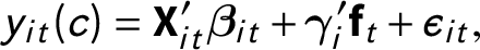 $$ \begin{align} y_{it} (c)&= \textbf{X}_{it}^{\prime}\boldsymbol{\beta}_{it} + \boldsymbol{\gamma}_{i}^{\prime}\textbf{f}_{t} + \epsilon_{it}, \end{align} $$
 $$ \begin{align} \boldsymbol{\beta}_{it} &= \boldsymbol{\beta} + \boldsymbol{\alpha}_{i} +\boldsymbol{\xi}_{t}, \end{align} $$
 $$ \begin{align} \boldsymbol{\xi}_{t} &= \Phi_{\xi} \boldsymbol{\xi}_{t - 1} + \boldsymbol{e}_{t}, \ \textbf{f}_{t} = \Phi_{f} \textbf{f}_{t - 1} + \boldsymbol{\nu}_{t}. \end{align} $$
Equation (5) is the individual-level regression, in which $y_{it}(c)$
is explained by three components. The first one,
$y_{it}(c)$
is explained by three components. The first one, $\textbf{X}_{it} \boldsymbol {\beta }_{it} $
, captures the relationships between observed covariates and the outcome. The double subscripts of
$\textbf{X}_{it} \boldsymbol {\beta }_{it} $
, captures the relationships between observed covariates and the outcome. The double subscripts of $\boldsymbol {\beta }_{it}$
indicate that we allow these relationships to be heterogeneous across units and over time. Equation (6) decomposes
$\boldsymbol {\beta }_{it}$
indicate that we allow these relationships to be heterogeneous across units and over time. Equation (6) decomposes $\boldsymbol {\beta }_{it}$
into three parts:
$\boldsymbol {\beta }_{it}$
into three parts: $\boldsymbol {\beta }$
is the mean of
$\boldsymbol {\beta }$
is the mean of $\boldsymbol {\beta }_{it}$
and shared by all observations, and
$\boldsymbol {\beta }_{it}$
and shared by all observations, and $\boldsymbol {\alpha }_{i}$
and
$\boldsymbol {\alpha }_{i}$
and $\boldsymbol {\xi }_{t}$
are zero-mean unit- and time-specific “residuals” of
$\boldsymbol {\xi }_{t}$
are zero-mean unit- and time-specific “residuals” of $\boldsymbol {\beta }_{it}$
, respectively. The second component,
$\boldsymbol {\beta }_{it}$
, respectively. The second component, $\boldsymbol {\gamma }_{i}^{\prime }\textbf{f}_{t} $
, is the multifactor term, in which
$\boldsymbol {\gamma }_{i}^{\prime }\textbf{f}_{t} $
, is the multifactor term, in which $\textbf{f}_{t}$
and
$\textbf{f}_{t}$
and $\boldsymbol {\gamma }_{i}$
are
$\boldsymbol {\gamma }_{i}$
are $(r\times 1)$
vectors of factors and factor loadings, respectively. Consistent with Assumption 5, we use
$(r\times 1)$
vectors of factors and factor loadings, respectively. Consistent with Assumption 5, we use $\textbf{f}_{t}$
and
$\textbf{f}_{t}$
and $\boldsymbol {\gamma }_{i}$
to approximate
$\boldsymbol {\gamma }_{i}$
to approximate $\textbf{U}_{i}$
. The last component,
$\textbf{U}_{i}$
. The last component, $\epsilon _{it}$
, represents
$\epsilon _{it}$
, represents $i.i.d.$
idiosyncratic errors. We further model the dynamics in
$i.i.d.$
idiosyncratic errors. We further model the dynamics in $\boldsymbol {\xi }_{t}$
and
$\boldsymbol {\xi }_{t}$
and $\textbf{f}_{t}$
by specifying autoregressive processes as shown in Equation (7). We assume both transition matrices
$\textbf{f}_{t}$
by specifying autoregressive processes as shown in Equation (7). We assume both transition matrices $\Phi _{\xi }$
and
$\Phi _{\xi }$
and $\Phi _{f}$
are diagonal:
$\Phi _{f}$
are diagonal: $\Phi _{\xi } = \textrm{Diag}(\phi _{\xi _{1}}, \ldots , \phi _{\xi _{p_{3}}}) $
and
$\Phi _{\xi } = \textrm{Diag}(\phi _{\xi _{1}}, \ldots , \phi _{\xi _{p_{3}}}) $
and $\Phi _{f} = \textrm{Diag}(\phi _{f_{1}}, \ldots , \phi _{f_{r}})$
.Footnote
2
Finally, we assume the individual- and group-level errors,
$\Phi _{f} = \textrm{Diag}(\phi _{f_{1}}, \ldots , \phi _{f_{r}})$
.Footnote
2
Finally, we assume the individual- and group-level errors, $\epsilon _{it}$
,
$\epsilon _{it}$
, $\boldsymbol {e}_{t}$
, and
$\boldsymbol {e}_{t}$
, and $\boldsymbol {\nu }_{t}$
, to be i.i.d. normal.
$\boldsymbol {\nu }_{t}$
, to be i.i.d. normal.
The DM-LFM allows the slope coefficient of each covariate to vary by unit, time, both, or neither. To illustrate this flexibility, we rewrite the individual-level model in a reduced and matrix format a s
 $$ \begin{align} \boldsymbol{y}_{i}(c) = \boldsymbol{X}_{i}\boldsymbol{\beta} + \boldsymbol{Z}_{i}\boldsymbol{\alpha}_{i} + \boldsymbol{A}_{i} \boldsymbol{\xi} + \textbf{F}\boldsymbol{\gamma}_{i} + \boldsymbol{\epsilon}_{i}, \end{align} $$
in which $\textbf {F} = (\textbf{f}_{1}, \ldots , \textbf{f}_{T})^{\prime }$
is a
$\textbf {F} = (\textbf{f}_{1}, \ldots , \textbf{f}_{T})^{\prime }$
is a $(T \times r)$
factor matrix.
$(T \times r)$
factor matrix. $\boldsymbol {Z}_{i}$
of dimension
$\boldsymbol {Z}_{i}$
of dimension $(T\times p_{2})$
are covariates that have unit-specific slopes (
$(T\times p_{2})$
are covariates that have unit-specific slopes ( $\boldsymbol {\beta }+\boldsymbol {\alpha }_{i}$
).
$\boldsymbol {\beta }+\boldsymbol {\alpha }_{i}$
). $\boldsymbol {A}_{i}$
of dimension
$\boldsymbol {A}_{i}$
of dimension $(T \times p_{3})$
are covariates that have time-specific slopes (
$(T \times p_{3})$
are covariates that have time-specific slopes ( $\boldsymbol {\beta }+\boldsymbol {\xi }_{t}$
). Both
$\boldsymbol {\beta }+\boldsymbol {\xi }_{t}$
). Both $\boldsymbol {A}_{i}$
and
$\boldsymbol {A}_{i}$
and $\boldsymbol {Z}_{i}$
are subsets of
$\boldsymbol {Z}_{i}$
are subsets of $\boldsymbol {X}_{i}$
. When the kth covariate is in
$\boldsymbol {X}_{i}$
. When the kth covariate is in $\boldsymbol {A}_{i} \cap \boldsymbol {Z}_{i}$
, it has a slope coefficient that varies across units and over time, that is,
$\boldsymbol {A}_{i} \cap \boldsymbol {Z}_{i}$
, it has a slope coefficient that varies across units and over time, that is, $\beta _{it}^{(k)} = \beta ^{(k)}+\alpha _{i}^{(k)}+\xi _{t}^{(k)}$
. Accordingly,
$\beta _{it}^{(k)} = \beta ^{(k)}+\alpha _{i}^{(k)}+\xi _{t}^{(k)}$
. Accordingly, $\boldsymbol {\beta }$
is a
$\boldsymbol {\beta }$
is a $(p_{1}\times 1)$
coefficients vector,
$(p_{1}\times 1)$
coefficients vector, $\boldsymbol {\alpha }_{i} $
is a
$\boldsymbol {\alpha }_{i} $
is a $(p_{2} \times 1)$
vector,
$(p_{2} \times 1)$
vector, $\boldsymbol {\xi } = (\boldsymbol {\xi }_{1}^{\prime }, \ldots , \boldsymbol {\xi }_{T}^{\prime })^{\prime }$
is a
$\boldsymbol {\xi } = (\boldsymbol {\xi }_{1}^{\prime }, \ldots , \boldsymbol {\xi }_{T}^{\prime })^{\prime }$
is a $(p_{3} \times 1)$
vector, and
$(p_{3} \times 1)$
vector, and $p_{1} \geqslant p_{2}, p_{3}$
. Because
$p_{1} \geqslant p_{2}, p_{3}$
. Because $\boldsymbol {\alpha }_{i}, \boldsymbol {\xi }_{t}, \textbf{f}_{t}$
are centered at zero, the systemic part of the model is
$\boldsymbol {\alpha }_{i}, \boldsymbol {\xi }_{t}, \textbf{f}_{t}$
are centered at zero, the systemic part of the model is $\mathbb{E}[\textbf {y}_{i}(c)]=\textbf{X}_{i}\boldsymbol {\beta }$
. The rest of the components define the variance of the composite errors as
$\mathbb{E}[\textbf {y}_{i}(c)]=\textbf{X}_{i}\boldsymbol {\beta }$
. The rest of the components define the variance of the composite errors as $\boldsymbol {\Omega }_{\textbf {y}_{i}(c)-\boldsymbol {X}_{i}\boldsymbol {\beta }} = (\boldsymbol {Z}_{i}\boldsymbol {\alpha }_{i} + \boldsymbol {A}_{i} \boldsymbol {\xi } + \textbf {F}\boldsymbol {\gamma }_{i})^{\prime }(\boldsymbol {Z}_{i}\boldsymbol {\alpha }_{i} + \boldsymbol {A}_{i} \boldsymbol {\xi } + \textbf {F}\boldsymbol {\gamma }_{i})+ \sigma ^{2}_{\epsilon }\textbf {I}$
, which contains nonzero off-diagonal elements because of the components
$\boldsymbol {\Omega }_{\textbf {y}_{i}(c)-\boldsymbol {X}_{i}\boldsymbol {\beta }} = (\boldsymbol {Z}_{i}\boldsymbol {\alpha }_{i} + \boldsymbol {A}_{i} \boldsymbol {\xi } + \textbf {F}\boldsymbol {\gamma }_{i})^{\prime }(\boldsymbol {Z}_{i}\boldsymbol {\alpha }_{i} + \boldsymbol {A}_{i} \boldsymbol {\xi } + \textbf {F}\boldsymbol {\gamma }_{i})+ \sigma ^{2}_{\epsilon }\textbf {I}$
, which contains nonzero off-diagonal elements because of the components $\textbf {Z}_{i}$
and
$\textbf {Z}_{i}$
and $\textbf {A}_{i}$
. Note that we allow
$\textbf {A}_{i}$
. Note that we allow $\boldsymbol {Z}_{i}\boldsymbol {\alpha }_{i}$
,
$\boldsymbol {Z}_{i}\boldsymbol {\alpha }_{i}$
, $\boldsymbol {A}_{i}\boldsymbol {\xi }$
, and
$\boldsymbol {A}_{i}\boldsymbol {\xi }$
, and $\textbf {F}\boldsymbol {\gamma }_{i}$
to be arbitrarily correlated.
$\textbf {F}\boldsymbol {\gamma }_{i}$
to be arbitrarily correlated.
Figure 1 presents the model graphically, and the shrinkage parameters $\lambda $
’s in the figure will be discussed later. Note that this outcome model governs
$\lambda $
’s in the figure will be discussed later. Note that this outcome model governs $y_{it}(c)$
only. Without loss of generality, we can add
$y_{it}(c)$
only. Without loss of generality, we can add $\delta _{it}w_{it} $
in the model in which
$\delta _{it}w_{it} $
in the model in which $\delta _{it}$
is the causal effect for unit i at time t. This model is a dynamic and multilevel extension to several existing causal inference methods with TSCS data. For example, if we set
$\delta _{it}$
is the causal effect for unit i at time t. This model is a dynamic and multilevel extension to several existing causal inference methods with TSCS data. For example, if we set $ \textbf {Z}_{i} = \textbf {A}_{i} = (1,1,\dots , 1)^{\prime }$
, and
$ \textbf {Z}_{i} = \textbf {A}_{i} = (1,1,\dots , 1)^{\prime }$
, and $ r = 0 $
, Equation (8) becomes a parametric linear DiD model with covariates and two-way fixed effects:
$ r = 0 $
, Equation (8) becomes a parametric linear DiD model with covariates and two-way fixed effects: $y_{it} = \delta _{it} w_{it} + \textbf{X}_{it}^{\prime } \boldsymbol {\beta } + \alpha _{i} + \xi _{t} + \epsilon _{it}$
. This is what Liu, Wang, and Xu (Reference Liu, Wang and Xu2020) call the fixed effects counterfactual model. When we put restrictions
$y_{it} = \delta _{it} w_{it} + \textbf{X}_{it}^{\prime } \boldsymbol {\beta } + \alpha _{i} + \xi _{t} + \epsilon _{it}$
. This is what Liu, Wang, and Xu (Reference Liu, Wang and Xu2020) call the fixed effects counterfactual model. When we put restrictions $\textbf {Z}_{it} = \varnothing $
and
$\textbf {Z}_{it} = \varnothing $
and $\textbf{X}_{i} = \textbf {A}_{i}$
is time-invariant, our model is reduced to a factor model that justifies the SCM (Abadie, Diamond, and Hainmueller Reference Abadie, Diamond and Hainmueller2010):
$\textbf{X}_{i} = \textbf {A}_{i}$
is time-invariant, our model is reduced to a factor model that justifies the SCM (Abadie, Diamond, and Hainmueller Reference Abadie, Diamond and Hainmueller2010): $y_{it} = \delta _{it} w_{it} + \xi _{t} + \textbf{X}_{i}^{\prime }\boldsymbol {\beta }_{t} + \boldsymbol {\gamma }_{i}^{\prime }\textbf{f}_{t} + \epsilon _{it}$
. Gsynth is also a special case of the model when we force the coefficients not to vary; that is,
$y_{it} = \delta _{it} w_{it} + \xi _{t} + \textbf{X}_{i}^{\prime }\boldsymbol {\beta }_{t} + \boldsymbol {\gamma }_{i}^{\prime }\textbf{f}_{t} + \epsilon _{it}$
. Gsynth is also a special case of the model when we force the coefficients not to vary; that is, $\textbf {Z}_{it} = \varnothing $
and
$\textbf {Z}_{it} = \varnothing $
and $\textbf {A}_{it} = \varnothing $
and
$\textbf {A}_{it} = \varnothing $
and $y_{it} = \delta _{it} w_{it} + \textbf{X}_{it}^{\prime }\boldsymbol {\beta } + \boldsymbol {\gamma }_{i}^{\prime }\textbf{f}_{t} + \epsilon _{it}$
(Xu Reference Xu2017).
$y_{it} = \delta _{it} w_{it} + \textbf{X}_{it}^{\prime }\boldsymbol {\beta } + \boldsymbol {\gamma }_{i}^{\prime }\textbf{f}_{t} + \epsilon _{it}$
(Xu Reference Xu2017).
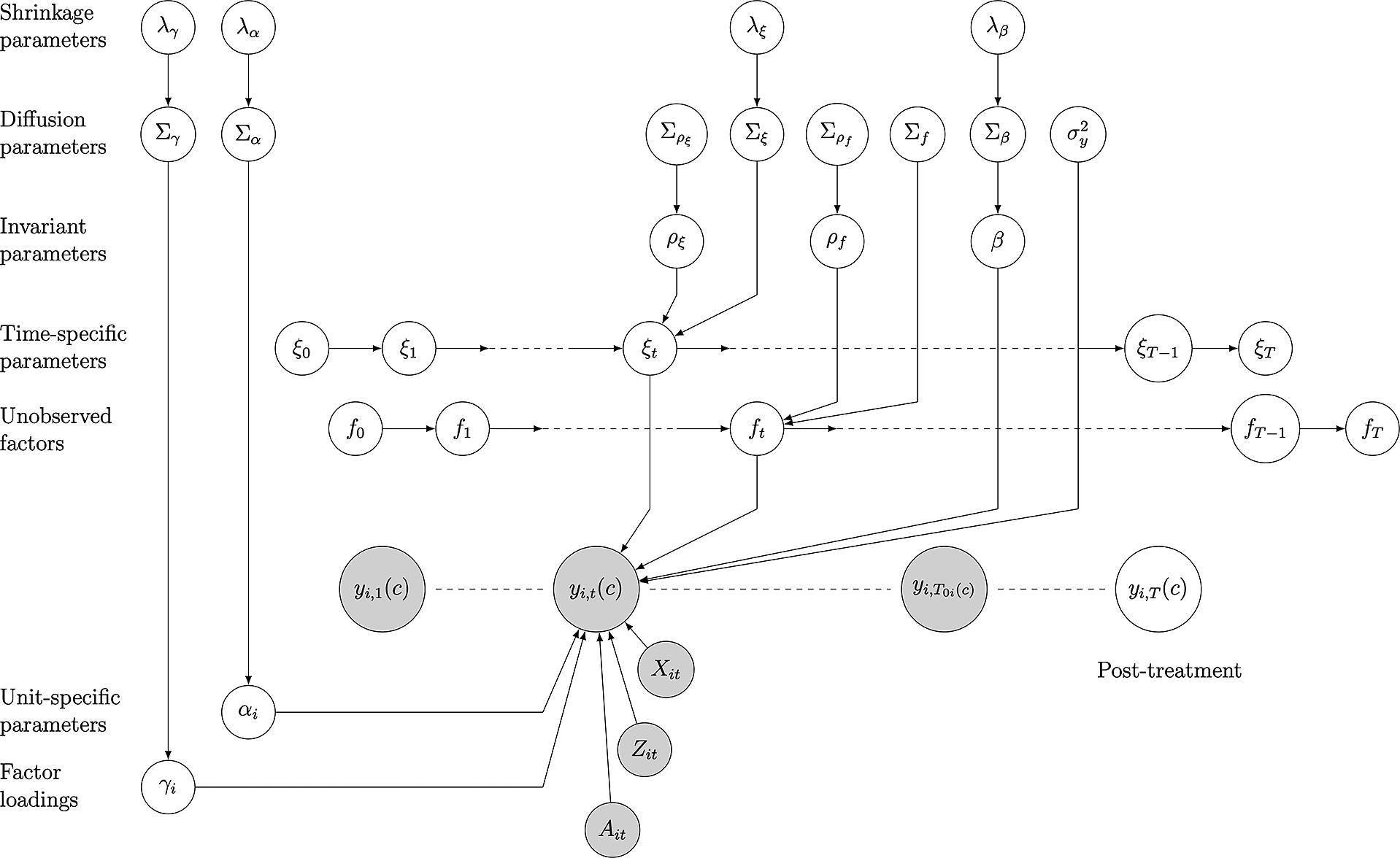
Figure 1 A graphic representation of dynamic multilevel latent factor model (DM-LFM). The shaded nodes represent observed data, including untreated outcomes and covariates; the unshaded nodes represent “missing” data (treated counterfactuals) and parameters. Only one (treated) unit i is shown. $T_{0i} = a_{i}-1$
is the last period before the treatment starts to affect unit i. The focus of the graph is Period t. Covariates in periods other than t, as well as relationships between parameters and
$T_{0i} = a_{i}-1$
is the last period before the treatment starts to affect unit i. The focus of the graph is Period t. Covariates in periods other than t, as well as relationships between parameters and $y_{i1}(c)$
,
$y_{i1}(c)$
, $y_{iT_{0i}(c)}$
, and
$y_{iT_{0i}(c)}$
, and $y_{iT}(c)$
, are omitted for simplicity.
$y_{iT}(c)$
, are omitted for simplicity.
3.2 Bayesian Stochastic Model Specification Search
One advantage of the DM-LFM is that it is highly flexible. However, the large number of specification options poses a challenge to model selection. Bayesian stochastic model searching reduces the risks of model mis-specification and simultaneously incorporates model uncertainty. We use shrinkage priors to choose the number of latent factors and decide whether and how to include a covariate. Specifically, we adopt the Bayesian Lasso and Lasso-like hierarchical shrinkage methods based on recent research.Footnote
3
We apply the Bayesian Lasso shrinkage on $\boldsymbol {\beta }$
using the following hierarchical setting of mixture of a normal-exponential prior,
$\boldsymbol {\beta }$
using the following hierarchical setting of mixture of a normal-exponential prior, $\beta _{k} | \tau _{\beta _{k}}^{2} \sim \mathcal {N}(0, \tau _{\beta _{k}}^{2}), \ \tau _{\beta _{k}}^{2} | \lambda _{\beta } \sim Exp(\frac {\lambda _{\beta }^{2}}{2}), \ \lambda _{\beta }^{2} \sim \mathcal {G}(a_{1}, a_{2}), \ k=1,\ldots , p_{1}$
. The tuning parameter
$\beta _{k} | \tau _{\beta _{k}}^{2} \sim \mathcal {N}(0, \tau _{\beta _{k}}^{2}), \ \tau _{\beta _{k}}^{2} | \lambda _{\beta } \sim Exp(\frac {\lambda _{\beta }^{2}}{2}), \ \lambda _{\beta }^{2} \sim \mathcal {G}(a_{1}, a_{2}), \ k=1,\ldots , p_{1}$
. The tuning parameter $\lambda $
controls the sparsity and degree of shrinkage and can be understood as the Bayesian equivalent to the regulation penalty in a frequentist Lasso regression. Instead of fixing
$\lambda $
controls the sparsity and degree of shrinkage and can be understood as the Bayesian equivalent to the regulation penalty in a frequentist Lasso regression. Instead of fixing $\lambda $
at a single value, we take advantage of Bayesian hierarchical modeling and give it a Gamma distribution with hyper-parameters
$\lambda $
at a single value, we take advantage of Bayesian hierarchical modeling and give it a Gamma distribution with hyper-parameters $a_{1}$
and
$a_{1}$
and $a_{2}$
.Footnote
4
$a_{2}$
.Footnote
4
To select the other components of the model, we impose shrinkage on $\boldsymbol {\alpha }_{i}$
,
$\boldsymbol {\alpha }_{i}$
, $\boldsymbol {\xi }_{t}$
, or
$\boldsymbol {\xi }_{t}$
, or $\boldsymbol {\gamma }_{i}$
to determine whether to include a
$\boldsymbol {\gamma }_{i}$
to determine whether to include a $Z_{j}$
(
$Z_{j}$
( $\,j = 1, 2, \dots , p_{2}$
),
$\,j = 1, 2, \dots , p_{2}$
), $A_{j}$
(
$A_{j}$
( $\,j = 1, 2, \dots , p_{3}$
), or
$\,j = 1, 2, \dots , p_{3}$
), or $f_{j}$
(
$f_{j}$
( $\,j = 1, 2, \dots , r$
) in the model. We consider the Lasso-like hierarchical shrinkage approach with re-parameterization. Assume
$\,j = 1, 2, \dots , r$
) in the model. We consider the Lasso-like hierarchical shrinkage approach with re-parameterization. Assume $\boldsymbol {\alpha }_{i}$
,
$\boldsymbol {\alpha }_{i}$
, $\boldsymbol {\gamma }_{i}$
, and
$\boldsymbol {\gamma }_{i}$
, and $\boldsymbol {\xi }_{t}$
have diagonal variance–covariance matrices,
$\boldsymbol {\xi }_{t}$
have diagonal variance–covariance matrices, $\textbf {H}_{0} = \textrm{Diag}(\omega _{\alpha _{1}}^{2}, \ldots , \omega _{\alpha _{p_{2}}}^{2}), \ \boldsymbol {\Gamma }_{0} = \textrm{Diag}(\omega _{\gamma _{1}}^{2}, \ldots , \omega _{\gamma _{r}}^{2}), \ \Sigma _{e} = \textrm{Diag}(\omega _{\xi _{1}}^{2}, \ldots , \omega _{\xi _{p_{3}}}^{2})$
, respectively. To have a shrinkage effect, we should allow the variance parameters
$\textbf {H}_{0} = \textrm{Diag}(\omega _{\alpha _{1}}^{2}, \ldots , \omega _{\alpha _{p_{2}}}^{2}), \ \boldsymbol {\Gamma }_{0} = \textrm{Diag}(\omega _{\gamma _{1}}^{2}, \ldots , \omega _{\gamma _{r}}^{2}), \ \Sigma _{e} = \textrm{Diag}(\omega _{\xi _{1}}^{2}, \ldots , \omega _{\xi _{p_{3}}}^{2})$
, respectively. To have a shrinkage effect, we should allow the variance parameters $\omega ^{2}$
to have a positive probability to take the value zero. Therefore, we re-parameterize
$\omega ^{2}$
to have a positive probability to take the value zero. Therefore, we re-parameterize $\boldsymbol {\alpha }_{i}$
,
$\boldsymbol {\alpha }_{i}$
, $\boldsymbol {\xi }_{t}$
, and
$\boldsymbol {\xi }_{t}$
, and $\boldsymbol {\gamma }_{i}$
as
$\boldsymbol {\gamma }_{i}$
as $\boldsymbol {\alpha }_{i}=\boldsymbol {\omega }_{\boldsymbol {\alpha }} \cdot \tilde {\boldsymbol {\alpha }}_{i},\ \boldsymbol {\xi }_{t} =\boldsymbol {\omega }_{\boldsymbol {\xi }} \cdot \tilde {\boldsymbol {\xi }}_{t}, \ \boldsymbol {\gamma }_{i}=\boldsymbol {\omega }_{\boldsymbol {\gamma }} \cdot \tilde {\boldsymbol {\gamma }}_{i}$
, where
$\boldsymbol {\alpha }_{i}=\boldsymbol {\omega }_{\boldsymbol {\alpha }} \cdot \tilde {\boldsymbol {\alpha }}_{i},\ \boldsymbol {\xi }_{t} =\boldsymbol {\omega }_{\boldsymbol {\xi }} \cdot \tilde {\boldsymbol {\xi }}_{t}, \ \boldsymbol {\gamma }_{i}=\boldsymbol {\omega }_{\boldsymbol {\gamma }} \cdot \tilde {\boldsymbol {\gamma }}_{i}$
, where $\boldsymbol {\omega }_{\alpha } = (\omega _{\alpha _{1}}, \ldots , \omega _{\alpha _{p_{2}}})^{\prime }$
,
$\boldsymbol {\omega }_{\alpha } = (\omega _{\alpha _{1}}, \ldots , \omega _{\alpha _{p_{2}}})^{\prime }$
, $\boldsymbol {\omega }_{\xi } = (\omega _{\xi _{1}}, \ldots , \omega _{\xi _{p_{3}}})^{\prime }$
, and
$\boldsymbol {\omega }_{\xi } = (\omega _{\xi _{1}}, \ldots , \omega _{\xi _{p_{3}}})^{\prime }$
, and $\boldsymbol {\omega }_{\gamma } = (\omega _{\gamma _{1}}, \ldots , \omega _{\gamma _{r}})^{\prime }$
are column vectors. After re-parameterization, the variances
$\boldsymbol {\omega }_{\gamma } = (\omega _{\gamma _{1}}, \ldots , \omega _{\gamma _{r}})^{\prime }$
are column vectors. After re-parameterization, the variances $\boldsymbol {\omega }^{2}$
appear in the model as coefficients
$\boldsymbol {\omega }^{2}$
appear in the model as coefficients $\boldsymbol {\omega }$
that can take values on the entire real line, and the new variance–covariance matrices become identity matrices.
$\boldsymbol {\omega }$
that can take values on the entire real line, and the new variance–covariance matrices become identity matrices.
Now we assign Lasso priors to each $\omega _{\alpha }$
,
$\omega _{\alpha }$
, $\omega _{\xi }$
, and
$\omega _{\xi }$
, and $\omega _{\gamma _{j}}$
to shrink varying parameters grouped by unit or time. Together with the shrinkage on
$\omega _{\gamma _{j}}$
to shrink varying parameters grouped by unit or time. Together with the shrinkage on $\boldsymbol {\beta }$
, the algorithm will decide de facto whether a certain covariate is included, whether its coefficient varies by time or across units, and how many latent factors are considered. Because the shrinkage priors do not have a point mass component at zero, parameters of less important covariates are not zeroed out completely. Instead, they stay in the model but with shrunk impacts and can be regarded as virtually excluded from the model. The posterior distribution of
$\boldsymbol {\beta }$
, the algorithm will decide de facto whether a certain covariate is included, whether its coefficient varies by time or across units, and how many latent factors are considered. Because the shrinkage priors do not have a point mass component at zero, parameters of less important covariates are not zeroed out completely. Instead, they stay in the model but with shrunk impacts and can be regarded as virtually excluded from the model. The posterior distribution of $\omega $
may be of different shapes. If it is clearly bimodal, it means that the associated parameter is included in the model; if it is close to unimodal and centered at zero, it means that the parameter is virtually excluded from the model; if, however, the posterior distribution of
$\omega $
may be of different shapes. If it is clearly bimodal, it means that the associated parameter is included in the model; if it is close to unimodal and centered at zero, it means that the parameter is virtually excluded from the model; if, however, the posterior distribution of $\omega $
has three or more modes, it indicates that the data do not provide decisive information on whether the corresponding covariate or factor is sufficiently important—in some iterations, the parameter escapes the shrinkage while in others, it is trapped in a narrow neighborhood around zero. In each MCMC iteration, the algorithm samples a model consisting of the parameters that successfully escape the shrinkage, and posterior distributions of parameters generated by the stochastic search algorithm are based on a mixture of models in a continuous model space. In other words, this variable selection process is also a model-searching and model-averaging process.Footnote
5
$\omega $
has three or more modes, it indicates that the data do not provide decisive information on whether the corresponding covariate or factor is sufficiently important—in some iterations, the parameter escapes the shrinkage while in others, it is trapped in a narrow neighborhood around zero. In each MCMC iteration, the algorithm samples a model consisting of the parameters that successfully escape the shrinkage, and posterior distributions of parameters generated by the stochastic search algorithm are based on a mixture of models in a continuous model space. In other words, this variable selection process is also a model-searching and model-averaging process.Footnote
5
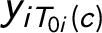
The DF-LFM has many parameters, but most of them, listed in Table 1(b), are included as part of Bayesian parameter expansion for computational convenience or as hyper-parameters to adjust for parameter uncertainties. They do not appear in the likelihood or can be integrated out of the likelihood given the effective parameters. The effective parameters, including $\boldsymbol {\beta }$
and the variance parameters, are reported in Table 1(a). Their number is usually much smaller than the number of observations.
$\boldsymbol {\beta }$
and the variance parameters, are reported in Table 1(a). Their number is usually much smaller than the number of observations.
Table 1. Total number of parameters.
The variance parameters for $\nu $
, e,
$\nu $
, e, $f_{t}$
do not appear in the table because we assume they have standard normal priors.
$f_{t}$
do not appear in the table because we assume they have standard normal priors.
3.3 Implementing a DM-LFM
We develop an MCMC algorithm to estimate a DM-LFM. The core functions of the algorithm is written in C++. Due to space limitations, we present the details of choices of priors and the iterative steps of MCMC updating in Section A.2 in online Supplementary Material. Broadly speaking, implementing a DM-LFM takes the following three steps:
Step 1. Model searching and parameter estimation. We specify and estimate the DM-FLM model with Bayesian shrinkage to sample G draws (excluding draws in the burn-in stage) of the parameters from their posterior distributions, $\boldsymbol {\theta }^{(g)}_{it} \sim \pi (\boldsymbol {\theta }_{it}| \mathfrak {D})$
, where
$\boldsymbol {\theta }^{(g)}_{it} \sim \pi (\boldsymbol {\theta }_{it}| \mathfrak {D})$
, where $\mathfrak {D}=\{(\textbf{X}_{it}, y_{it}(c)^{obs}): it \in S_{0}\}$
is the set of untreated observations. Because of Bayesian shrinkage,
$\mathfrak {D}=\{(\textbf{X}_{it}, y_{it}(c)^{obs}): it \in S_{0}\}$
is the set of untreated observations. Because of Bayesian shrinkage, $\pi (\boldsymbol {\theta }_{it}| \mathfrak {D})$
is in effect a mixture of distributions.
$\pi (\boldsymbol {\theta }_{it}| \mathfrak {D})$
is in effect a mixture of distributions.
Step 2. Prediction and integration. We conduct Bayesian prediction by generating draws of counterfactual $y_{it}(c)^{mis}$
for each treated unit at
$y_{it}(c)^{mis}$
for each treated unit at $a_{i} \leqslant t \leqslant T$
from its posterior predictive distribution:
$a_{i} \leqslant t \leqslant T$
from its posterior predictive distribution: $f(y_{it}(c)^{mis}|\textbf{X}, \textbf {Y}(\textbf {0})^{obs}) \propto \int f(y_{it}(c)^{mis}|\textbf{X}_{it}, \boldsymbol {\theta }_{it}) \pi (\boldsymbol {\theta }_{it}|\mathfrak {D})d\boldsymbol {\theta }_{it}$
. Bayesian prediction is an empirical integration: a sample of the predicted counterfactual is generated by plugging each draw
$f(y_{it}(c)^{mis}|\textbf{X}, \textbf {Y}(\textbf {0})^{obs}) \propto \int f(y_{it}(c)^{mis}|\textbf{X}_{it}, \boldsymbol {\theta }_{it}) \pi (\boldsymbol {\theta }_{it}|\mathfrak {D})d\boldsymbol {\theta }_{it}$
. Bayesian prediction is an empirical integration: a sample of the predicted counterfactual is generated by plugging each draw $\boldsymbol {\theta }^{(g)}_{it}$
from
$\boldsymbol {\theta }^{(g)}_{it}$
from $\pi (\boldsymbol {\theta }_{it}| \mathfrak {D})$
into
$\pi (\boldsymbol {\theta }_{it}| \mathfrak {D})$
into $f(y_{it}(c)^{mis}|\textbf{X}_{it}, \boldsymbol {\theta }_{it})$
to obtain
$f(y_{it}(c)^{mis}|\textbf{X}_{it}, \boldsymbol {\theta }_{it})$
to obtain $y^{(g)}_{it}(c)$
for
$y^{(g)}_{it}(c)$
for $g=1,\ldots , G$
. The sample of counterfactuals is drawn from
$g=1,\ldots , G$
. The sample of counterfactuals is drawn from $f(y_{it}(c)^{mis}|\textbf{X}_{it},\mathfrak {D} )= f(y_{it}(c)^{mis}|\textbf{X}, \textbf {Y}^{obs}(\textbf {0}))$
without any unknown quantities.
$f(y_{it}(c)^{mis}|\textbf{X}_{it},\mathfrak {D} )= f(y_{it}(c)^{mis}|\textbf{X}, \textbf {Y}^{obs}(\textbf {0}))$
without any unknown quantities.
Step 3. Inference and diagnostics. We make inference about the causal effect $\delta _{it}$
at
$\delta _{it}$
at $a_{i} \leqslant t \leqslant T$
for each treated unit i, by summarizing the empirical posterior distribution
$a_{i} \leqslant t \leqslant T$
for each treated unit i, by summarizing the empirical posterior distribution $\delta _{it}$
formed by
$\delta _{it}$
formed by $\delta ^{(g)}_{it} = y_{it}(a_{i}) - y^{(g)}_{it}(c), \ g=1,\ldots G $
. To summarize the results, we can obtain its posterior mean, variance, and the Bayesian 95% credibility interval. We can make inferences about other estimands, such as the ATT, by pooling the posterior draws of
$\delta ^{(g)}_{it} = y_{it}(a_{i}) - y^{(g)}_{it}(c), \ g=1,\ldots G $
. To summarize the results, we can obtain its posterior mean, variance, and the Bayesian 95% credibility interval. We can make inferences about other estimands, such as the ATT, by pooling the posterior draws of $\delta _{it}$
and summarizing their posterior distributions accordingly. We conduct Bayesian diagnostic tests on the convergence and mixing on main parameters’ posterior distributions and find that the MCMC algorithm converges fast and mixes well in our simulation and empirical studies.
$\delta _{it}$
and summarizing their posterior distributions accordingly. We conduct Bayesian diagnostic tests on the convergence and mixing on main parameters’ posterior distributions and find that the MCMC algorithm converges fast and mixes well in our simulation and empirical studies.
4 Simulation Studies
In this section, we first illustrate how the Bayesian DM-LFM works using a simulated example. We then study its properties by varying sample sizes and model specifications and compare its relative performance against existing methods, including SCM and Gsynth, in the case of a single treated unit. We report more findings from Monte Carlo exercises in Supplementary Material.
4.1 A Simulated Example
We simulate a panel dataset of 50 units and 30 time periods based on the following DGP:
 $$ \begin{align} y_{it} = \delta_{it}w_{it} + \textbf{X}_{it}^{\prime}\boldsymbol{\beta}_{it} + {\boldsymbol{\gamma}}_{i}^{\prime} \textbf{f}_{t} + \epsilon_{it} = \delta_{it}w_{it} + \textbf{X}_{it}^{\prime}(\boldsymbol{\beta}+\boldsymbol{\alpha}_{i}+\boldsymbol{\xi}_{t}) + {\boldsymbol{\gamma}}_{i}^{\prime} \textbf{f}_{t} + \epsilon_{it} \end{align} $$
in which $w_{it}$
is the treatment indicator and
$w_{it}$
is the treatment indicator and $\delta _{it}$
is the treatment effect.
$\delta _{it}$
is the treatment effect. $\textbf{X}_{it}$
is a vector of 10 covariates including an intercept and nine time-varying variables, but only the intercept and the first three covariates have nonzero, unit- and time-varying coefficients. We re-parameterize Equation (9) as
$\textbf{X}_{it}$
is a vector of 10 covariates including an intercept and nine time-varying variables, but only the intercept and the first three covariates have nonzero, unit- and time-varying coefficients. We re-parameterize Equation (9) as $y_{it} = \delta _{it}w_{it} + \textbf{X}_{it}^{\prime }\boldsymbol {\beta } + \textbf{X}_{it}^{\prime } ( {\boldsymbol {\omega }}_{\boldsymbol {\alpha }} \cdot \tilde {\boldsymbol {\alpha }}_{i}) + \textbf{X}_{it}^{\prime } ( {\boldsymbol {\omega }}_{\textbf {x}} \cdot \tilde {\boldsymbol {\xi }}_{t}) + ({\boldsymbol {\omega }}_{\boldsymbol {\gamma }} \cdot \tilde {\boldsymbol {\gamma }}_{i})^{\prime } \textbf{f}_{t} + \epsilon _{it}$
such that
$y_{it} = \delta _{it}w_{it} + \textbf{X}_{it}^{\prime }\boldsymbol {\beta } + \textbf{X}_{it}^{\prime } ( {\boldsymbol {\omega }}_{\boldsymbol {\alpha }} \cdot \tilde {\boldsymbol {\alpha }}_{i}) + \textbf{X}_{it}^{\prime } ( {\boldsymbol {\omega }}_{\textbf {x}} \cdot \tilde {\boldsymbol {\xi }}_{t}) + ({\boldsymbol {\omega }}_{\boldsymbol {\gamma }} \cdot \tilde {\boldsymbol {\gamma }}_{i})^{\prime } \textbf{f}_{t} + \epsilon _{it}$
such that $\tilde {\boldsymbol {\alpha }}_{i}$
,
$\tilde {\boldsymbol {\alpha }}_{i}$
, $\tilde {\boldsymbol {\xi }}_{t}$
, and
$\tilde {\boldsymbol {\xi }}_{t}$
, and $\tilde {\boldsymbol {\gamma }}_{i}$
all have univariances. Seven units receive the treatment starting from Period 21 and remain treated till Period 30. The remaining 23 units are never treated. The heterogeneous treatment effects are governed by
$\tilde {\boldsymbol {\gamma }}_{i}$
all have univariances. Seven units receive the treatment starting from Period 21 and remain treated till Period 30. The remaining 23 units are never treated. The heterogeneous treatment effects are governed by $\delta _{it,t>20}= t -20+ \tau _{it}$
, in which
$\delta _{it,t>20}= t -20+ \tau _{it}$
, in which $\tau _{it}\stackrel {i.i.d.}{\sim } N(0,1)$
. This means the expected value of the treatment effect gradually increases as the treatment duration grows, for example, from 1 in Period 21 to 10 in Period 30. The factor vector
$\tau _{it}\stackrel {i.i.d.}{\sim } N(0,1)$
. This means the expected value of the treatment effect gradually increases as the treatment duration grows, for example, from 1 in Period 21 to 10 in Period 30. The factor vector $\textbf{f}_{t}$
is two-dimensional and both factors follow an AR(1) process. The probability of getting treated is positively correlated with the sum of a unit’s factor loadings
$\textbf{f}_{t}$
is two-dimensional and both factors follow an AR(1) process. The probability of getting treated is positively correlated with the sum of a unit’s factor loadings $\tilde {\boldsymbol {\gamma }}_{i}$
, which are also i.i.d.
$\tilde {\boldsymbol {\gamma }}_{i}$
, which are also i.i.d. $N(0,1)$
. The selection on the factor loadings will cause biases in the causal estimates if a model does not account for the factor term or the covariates. We provide the details of the DGP in Supplementary Material.
$N(0,1)$
. The selection on the factor loadings will cause biases in the causal estimates if a model does not account for the factor term or the covariates. We provide the details of the DGP in Supplementary Material.
Figure 2 shows the estimated ATT (posterior means) with their 95% credibility intervals using a Bayesian DiD model (a) and a DM-LFM model (b). The DiD model assumes $\boldsymbol {\omega }_{\boldsymbol {\alpha }}=\boldsymbol {\omega }_{\boldsymbol {\xi }}=\boldsymbol {\omega }_{\boldsymbol {\gamma }}=0$
; in other words, the coefficients for the covariates are assumed to be constant, and no factors are included in the model. Figure 2(a) shows that with the DiD estimator, multiple estimates in the pre-treatment periods are away from zero and significant biases exist for the ATT estimates in the post-treatment periods. On the contrary, the DM-LFM performs significantly better: we do not observe any pre-trend and the ATT estimates are close to the true values, which are covered by the corresponding 95% credibility intervals.
$\boldsymbol {\omega }_{\boldsymbol {\alpha }}=\boldsymbol {\omega }_{\boldsymbol {\xi }}=\boldsymbol {\omega }_{\boldsymbol {\gamma }}=0$
; in other words, the coefficients for the covariates are assumed to be constant, and no factors are included in the model. Figure 2(a) shows that with the DiD estimator, multiple estimates in the pre-treatment periods are away from zero and significant biases exist for the ATT estimates in the post-treatment periods. On the contrary, the DM-LFM performs significantly better: we do not observe any pre-trend and the ATT estimates are close to the true values, which are covered by the corresponding 95% credibility intervals.
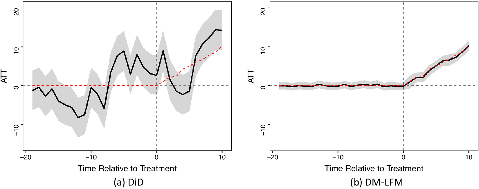
Figure 2 Estimated average treatment effect on the treated (ATT): difference-in-differences (DiD) versus dynamic multilevel latent factor model (DM-LFM). The above figures show the ATT estimates and their 95% credibility intervals from the DiD and DM-LFM estimators, both implemented with Bayesian Markov Chain Monte Carlo (MCMC) algorithms. The red dashed lines represent the true ATT of the five treated units.
Figure 3(a) and Figure 3(b) show the invariant and time-varying components of the covariate coefficients, respectively. While $\boldsymbol {\beta }$
and
$\boldsymbol {\beta }$
and $\boldsymbol {\xi }_{t}$
for the intercept and the first three covariates are clearly nonzero, the coefficients for the other six covariates are close to zero, which is consistent with the DGP. The algorithm also correctly selects the non-zero
$\boldsymbol {\xi }_{t}$
for the intercept and the first three covariates are clearly nonzero, the coefficients for the other six covariates are close to zero, which is consistent with the DGP. The algorithm also correctly selects the non-zero $\boldsymbol {\alpha }_{i}$
, the unit-varying components of coefficients (reported in Supplementary Material). Figure 3c shows the posterior distributions of
$\boldsymbol {\alpha }_{i}$
, the unit-varying components of coefficients (reported in Supplementary Material). Figure 3c shows the posterior distributions of $\boldsymbol {\omega }_{\gamma }$
, which measures the relative importance of each of the 10 factors subject to selection. It shows that two factors (Factors 1 and 2) have a
$\boldsymbol {\omega }_{\gamma }$
, which measures the relative importance of each of the 10 factors subject to selection. It shows that two factors (Factors 1 and 2) have a $\omega $
with clear bimodal posteriors, and the others all have spike-shaped unimodal ones. This means that the model correctly identifies the number of factors to be two.
$\omega $
with clear bimodal posteriors, and the others all have spike-shaped unimodal ones. This means that the model correctly identifies the number of factors to be two.

Figure 3 Posterior distributions of coefficients. (a) and (b) show the posterior mean and 95% credibility intervals of the invariant component and time-varying component of $\boldsymbol {\beta }_{it}$
, respectively. (c) shows the posterior distribution of each
$\boldsymbol {\beta }_{it}$
, respectively. (c) shows the posterior distribution of each $\boldsymbol {\omega }_{\boldsymbol {\gamma }}$
, which captures the extent to which a factor influences the outcome.
$\boldsymbol {\omega }_{\boldsymbol {\gamma }}$
, which captures the extent to which a factor influences the outcome.
This simulated example demonstrates that the DM-LFM performs well even when the sample size is relatively small and when researchers have limited knowledge about which covariates to put in, whether the covariates’ relationships with the outcome change over time or across units, or how many latent factors to include in the model.
4.2 Additional Monte Carlo Evidence
In addition, we conduct several sets of Monte Carlo exercises to study the properties of the proposed method and compare its relative performance against existing methods. Due to space limitations, we provide the details of these exercises in Supplementary Material and only briefly summarize two exercises and the major findings below.
In the first exercise, we study the role of each of the main components of a DM-LFM in estimation and investigate how the sample size affects the model performance. We simulate samples using the DGP as in Equation (9) while varying the sample size (both the total number of units N and the number of pre-treatment periods $T_{0}$
). We estimate and compare the full DM-LFM model with its three simpler variants: a model with covariates but without factors, analogous to a DiD model including covariates with fixed coefficients; a model without covariates but with 10 latent factors, analogous to Gsynth without time-varying covariates; and a model with factors and covariates with fixed coefficients. Figure 4 shows the comparison when the number of units is relatively small (
$T_{0}$
). We estimate and compare the full DM-LFM model with its three simpler variants: a model with covariates but without factors, analogous to a DiD model including covariates with fixed coefficients; a model without covariates but with 10 latent factors, analogous to Gsynth without time-varying covariates; and a model with factors and covariates with fixed coefficients. Figure 4 shows the comparison when the number of units is relatively small ( $N=40$
), and the full results are reported in Supplementary Material. In general, we find that DM-LFM outperforms the other three models in terms of bias, standard deviation, root mean squared errors (RMSE), and coverage. This exercise demonstrates that each of the key components of the model contributes to improving performance in causal effect estimation. The factor term seems to have the most impact, but covariates with varying coefficients also notably improve precision and coverage.
$N=40$
), and the full results are reported in Supplementary Material. In general, we find that DM-LFM outperforms the other three models in terms of bias, standard deviation, root mean squared errors (RMSE), and coverage. This exercise demonstrates that each of the key components of the model contributes to improving performance in causal effect estimation. The factor term seems to have the most impact, but covariates with varying coefficients also notably improve precision and coverage.
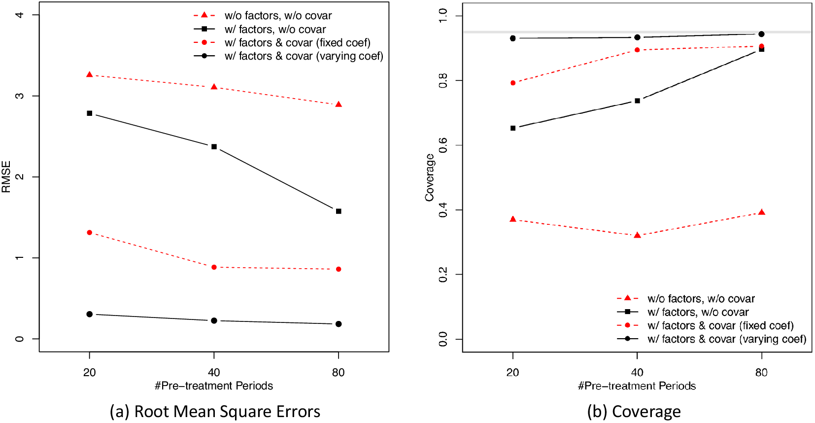
Figure 4 Comparison of model performance: root mean square errors (RMSE) and coverage. The above figures show the RMSE (a) and the coverage rate of 95% credibility intervals (b) of the average treatment effect on the treated (ATT) estimates using three sets of models: (1) models that do not include factors or covariates; (2) models that include 10 factors but no covariates; (3) models that include 10 factors and covariates with fixed coefficients; and (4) models that include 10 factors and covariates with varying coefficients.
The second exercise compares the performance of the DM-LFM with SCM and Gsynth in the case of a single treated unit. Tables A5–A7 in Supplementary Material show that, compared with the SCM, the DM-LFM has a much smaller RMSE. The DM-LFM outperforms Gsynth in the realistic scenario when the true number of factors is unknown, and when the number of factors is large and each of them produces relatively weak signals. Note that our Bayesian approach becomes significantly more computationally demanding as the sample size grows. For example, in one simulation in which $N= 50$
and
$N= 50$
and $T_{0}=60$
, it takes about 30 seconds to run a DM-LFM on a 2019 6-core MacBook Pro while Gsynth takes less than a second.
$T_{0}=60$
, it takes about 30 seconds to run a DM-LFM on a 2019 6-core MacBook Pro while Gsynth takes less than a second.
5 Empirical Applications
We apply the Bayesian DM-LFM to the two running examples introduced earlier. To gain confidence that the DM-LFM is appropriate for an application, we recommend users conduct the following diagnostic tests after running the model: (1) conduct Bayesian diagnostic tests on convergence and mixing of the MCMC output of key parameters, for example, by plotting of the traces of estimates; (2) examine whether the model fits the pre-treatment outcome trajectories of the treated units reasonably well; and (3) conduct a placebo test using pre-treatment data of the treated units when there is a sufficient number of pre-treatment periods for the treated units.
5.1 Economic Impact of German Reunification
First, we build a DM-LFM incorporating all pre-treatment time-invariant covariates considered in ADH (Reference Abadie, Diamond and Hainmueller2015), including pre-treatment averages of trade openness, inflation rate, industry share, schooling, and investment rate. The initial model we consider is $y_{it}(c) = \textbf{X}_{i}(\boldsymbol {\beta } + \boldsymbol {\xi }_{t}) + \textbf{f}_{t}\boldsymbol {\gamma }_{i} + .pngilon _{it}$
, in which
$y_{it}(c) = \textbf{X}_{i}(\boldsymbol {\beta } + \boldsymbol {\xi }_{t}) + \textbf{f}_{t}\boldsymbol {\gamma }_{i} + .pngilon _{it}$
, in which $\textbf{X}_{i}$
represents the time-invariant covariates. We do not include unit fixed effects or unit-varying coefficients to be consistent with the SCM, but time-varying coefficients are included. Figure A3 in Supplementary Material shows that the intercept has a strong time trend, but all the covariate coefficients are almost constant over time. Our result suggests four to six factors, with their
$\textbf{X}_{i}$
represents the time-invariant covariates. We do not include unit fixed effects or unit-varying coefficients to be consistent with the SCM, but time-varying coefficients are included. Figure A3 in Supplementary Material shows that the intercept has a strong time trend, but all the covariate coefficients are almost constant over time. Our result suggests four to six factors, with their $\omega $
’s clearly having bimodal posteriors while several other factors exhibit mixed posteriors (Figure A4 in Supplementary Material).
$\omega $
’s clearly having bimodal posteriors while several other factors exhibit mixed posteriors (Figure A4 in Supplementary Material).
We then produce an empirical posterior distribution of GDP per capita for counterfactual West Germany had German reunification not happened. To check the goodness-of-fit, we also calculate the model prediction of its GDP per capita in pre-treatment years. In Figure 5, we compare the counterfactual predictions of the SCM (a) with that of the DM-LFM (b), in which we shade the 95% Bayesian credibility intervals in gray. The dashed vertical line indicates the year 1989, 1 year before the adoption time. The two methods yield similar results: the GDP per capita of the counterfactual West Germany is higher than that of the actual West Germany during most of the post-reunification period except for the first few years after reunification.

Figure 5 Actual and estimated counterfactuals for West Germany. This figure shows the per capita gross domestic product (GDP) of actual West Germany and the posterior means (with 95% credibility intervals) of its untreated outcome from 1960 to 2003. The within-sample prediction is very precise and the interval is too narrow to be seen in the figure between 1960 and 1989.
Finally, we draw inferences about the treatment effects. Figure 6(a) and Figure 6(b) report the estimated effects of reunification on West Germany using the SCM and Bayesian DM-LFM, respectively. The corresponding 95% credibility intervals are added in (b). To lend further credibility to our causal estimates, we conduct a placebo test by setting 1987–1989, 3 years before reunification, as the placebo period. Figure 6(c) shows that the estimated effects at each time point during the placebo period are close to 0, buttressing our confidence in the identification assumptions.
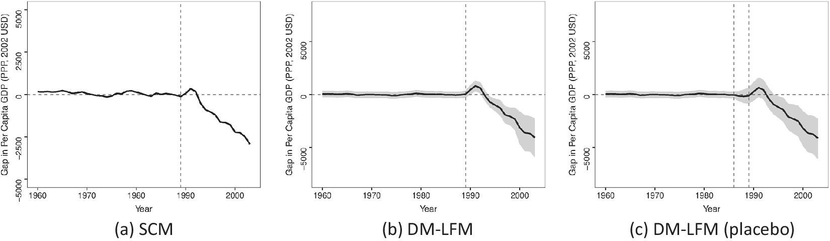
Figure 6 Estimated effect of reunification on West Germany. This figure shows the estimated treatment effect of reunification on West Germany’s per capita gross domestic product (GDP) using the synthetic control method (SCM) (a) and dynamic multilevel latent factor model (DM-LFM) (b), as well as the result from a placebo test using DM-LFM in which the 1987–1989 period (before reunification) is taken as “treated” (c).
5.2 Election Day Registration and Voter Turnout
For this example, we specify a full DM-LFM model including the same time-varying covariates used in Xu (Reference Xu2017) (universal mail-in registration and motor voter registration) as well as 10 factors. Because there are only two covariates, we do not impose shrinkage on their $\boldsymbol {\beta }$
, but assign shrinkage priors to
$\boldsymbol {\beta }$
, but assign shrinkage priors to $\boldsymbol {\alpha }_{i}$
,
$\boldsymbol {\alpha }_{i}$
, $\boldsymbol {\xi }_{t}$
, and
$\boldsymbol {\xi }_{t}$
, and $\boldsymbol {\gamma }_{i}$
. Our result suggests that at least six factors affect outcome prediction (Figure A9 in Supplementary Material). In contrast, Gsynth only includes two factors using a leave-one-out cross-validation procedure. As for
$\boldsymbol {\gamma }_{i}$
. Our result suggests that at least six factors affect outcome prediction (Figure A9 in Supplementary Material). In contrast, Gsynth only includes two factors using a leave-one-out cross-validation procedure. As for $\boldsymbol {\alpha }_{i}$
and
$\boldsymbol {\alpha }_{i}$
and $\boldsymbol {\xi }_{t}$
, the intercept varies in both time and space dimensions, but the varying parts of the slopes of the covariates are virtually shrunk to zero. We estimate the parameters using MCMC. Consistent with Xu (Reference Xu2017), we find that the two covariates do not explain much of the variation in turnout.
$\boldsymbol {\xi }_{t}$
, the intercept varies in both time and space dimensions, but the varying parts of the slopes of the covariates are virtually shrunk to zero. We estimate the parameters using MCMC. Consistent with Xu (Reference Xu2017), we find that the two covariates do not explain much of the variation in turnout.
We then generate the posterior distributions of counterfactual outcomes for the nine treated states in their post-treatment years, based on which we estimate the effect of EDR on voter turnout. In Figure 7, we report the ATT for the same duration of adoption. To do so, we pool the posterior draws of the individual treatment effects of all treated states in $p^{th}$
year after adoption for
$p^{th}$
year after adoption for $p = 1, 2, \dots , 6$
. Using the posterior distributions of
$p = 1, 2, \dots , 6$
. Using the posterior distributions of $\hat {\delta }_{p}$
, we obtain their posterior means and Bayesian 95% credibility intervals.
$\hat {\delta }_{p}$
, we obtain their posterior means and Bayesian 95% credibility intervals.
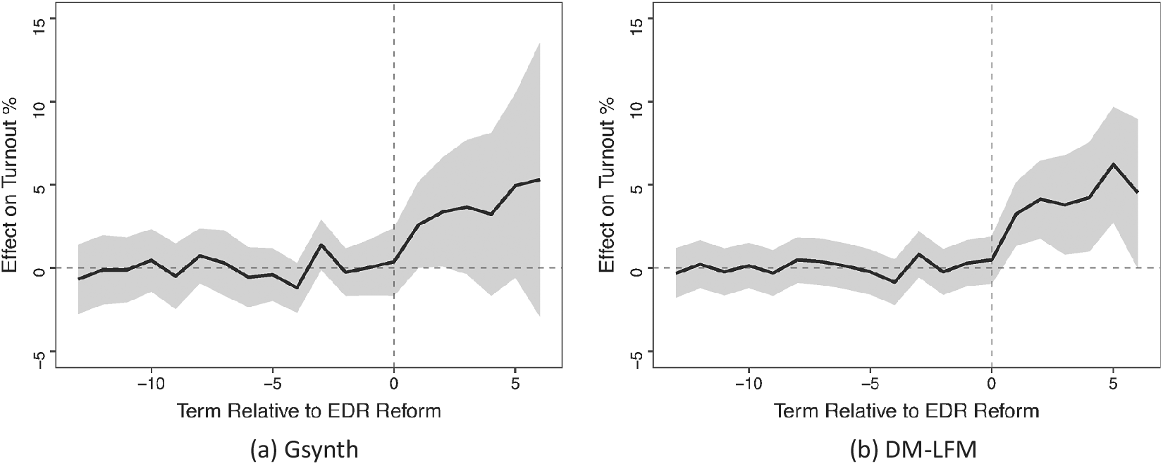
Figure 7 The effect of election day registration (EDR) on voter turnout. This figure shows the estimated average treatment effect of EDR on voter turnout in the United States using Gsynth (Xu Reference Xu2017) (a) and dynamic multilevel latent factor model (DM-LFM) (b), respectively. On the x-axis, the positive integers indicate the duration of treatment while the pre-treatment years are labeled as nonpositive integers. Period 1 is the first presidential election year in which a state implements EDR. Because the treated states adopted EDR at different points in time, the number of treated units decreases as p increases.
Comparing the point and uncertainty estimates up to the sixth post-adoption presidential elections from Gsynth and the DM-LFM, the most notable difference between them is that the Bayesian 95% credibility intervals are considerably narrower than the 95% confidence intervals from Gsynth. We suspect that this is because our Bayesian approach has better predictive performance of individual counterfactuals than Gsynth as evidenced in Figure A11 in Supplementary Material, where we report the individual treatment effects on six treated states that have at least three post-treatment measures of the outcome using both Gsynth and the DM-LFM—our new method fits the trajectory of each treated unit in the pre-treatment period noticeably better than Gsynth.
6 Discussion
When is the DM-LFM applicable? And when is it more advantageous than existing methods? Table 2 summarizes its features in comparison to those of DiD, SCM, and Gsynth. The most important differences among the methods, we acknowledge, is that DiD and SCM adopt a clear design-based perspective and rely on more transparent identification assumptions—these assumptions are not necessarily weak, but they are widely understood and accepted by researchers. Moreover, the weights they impose on control units—uniform weights in DiD designs and non-negative weights with the SCM—are directly interpretable. Gsynth (a frequentist LFM) and Bayesian DM-LFM, on the other hand, use a model-based approach. Together with the SCM, they address potential failures of the “parallel trends” assumption by assuming a linear factor model. Unlike the SCM, they can easily accommodate comparative case studies with multiple treated units.
Table 2. Comparing TSCS methods for comparative case studies.
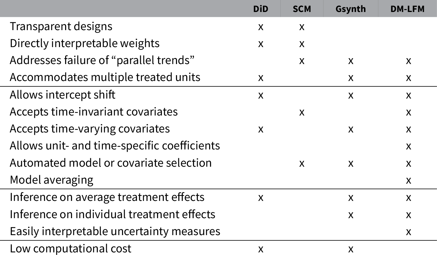
On modeling choices, DiD, Gsynth, and the DM-LFM allow intercept shift by assuming unit fixed effects, while the SCM does not (Doudchenko and Imbens Reference Doudchenko and Imbens2017). The SCM can accept only time-invariant covariates while DiD and Gsynth can accept only time-varying ones. The DM-LFM, however, can accommodate both types of covariates and allow their coefficients to vary by unit and time. In terms of model selection, the SCM uses held-out pre-treatment periods to tweak the weighting matrix; Gsynth uses a cross-validation scheme to select the number of factors; and the DM-LFM conducts model selection scholastically in a larger model space and averages model predictions simultaneously.
All in all, the Bayesian DM-LFM is especially well suited for comparative case study, particularly when researchers suspect the conventional “parallel trends” assumption is unlikely to hold; when there are multiple treated units; when researchers would like to have easily interpretable uncertainty estimates on average or individual treatment effects; when many pre-treatment covariates are available and their relationships with the outcome are complex; or when time-varying confounders are complex and/or subtle enough that they need a relatively large number of factors to represent or some of the factors are relatively weak. The biggest disadvantage of the Bayesian approach is that it is computationally more expensive than frequentist methods such as Gsynth when the sample size is large. We also find that the frequentist properties of our method are unsatisfactory when there are too few control units or the number of pre-treatment periods is too small, for example, $T_{0} < 20$
(see Table A4 in Supplementary Material).
$T_{0} < 20$
(see Table A4 in Supplementary Material).
Because of the strengths and weaknesses of different methods, we recommend researchers use multiple methods at the same time whenever possible to triangulate their findings. Future research should consider extending the method beyond the setting of staggered adoption, jointly modeling the treatment assignment mechanism and the response surface, and addressing potential SUTVA violations, such as policy diffusion and spillover effects.
Acknowledgements
We thank Dmitry Arkhangelsky, Neal Beck, Matt Blackwell, Sid Chib, Naoki Egami, Avi Feller, Matt Gabel, Jeff Gill, Kosuke Imai, Gary King, Dean Knox, John Londregan, Jacob Montgomery, Santiago Olivella, Jong Hee Park, Kevin Quinn, Marc Ratkovic, Guillermo Rosas, Betsy Sinclair, James F. Spriggs, Brandon Steward, Rocío Titiunik, Luwei Ying, Xiang Zhou, and participants at the Stanford Online Causal Inference Seminar, Annual Meeting of the Society for Political Methodology, the Harvard Applied Statistics Workshop, the Quantitative Social Science Colloquium at Princeton, and the workshop on “Frontiers of Bayesian Inference in Political Science” at Washington University in St. Louis. We are especially grateful to Associate Editor Dan Hopkins and three anonymous reviewers for their incredibly helpful comments. We thank Liz Crooks for excellent preproduction copy-editing. These authors contributed equally to this work and have decided to rotate the order of authorship in this and future collaborations.
Funding
This research is supported by the National Social Science Foundation of China (Grant No. 17ZDA110) as well as Stanford University.
Data Availability Agreement
Replication data and code for this article has been published at Harvard Dataverse at https://doi.org/10.7910/DVN/B6SWA1.
Supplementary Material
For supplementary material accompanying this paper, please visit https://doi.org/10.1017/pan.2021.22.


 Open access