


Introduction
When designing protective measures against snow avalanches it is generally necessary to predict the dynamical characteristics (height, length and velocity) of potential events threatening the considered site. Typical examples include the dimensioning of arrest dams against avalanches of large return periods (Reference Faug, Naaim and Naaim-BouvetFaug and others, 2004; Reference Naaim-Bouvet, Naaim and FaugNaaim-Bouvet and others, 2004; Reference Naaim, Faug, Naaim and EckertNaaim and others, 2010) and the establishment of hazard maps based on pressure thresholds. Physically based numerical models for the propagation of snow avalanches have made great advances in recent years, and are now able to address such issues with remarkable accuracy (Reference Barbolini, Gruber, Keylock, Naaim and SaviBarbolini and others, 2000; Reference Naaim, Naaim-Bouvet, Faug and BouchetNaaim and others, 2004; Reference Sovilla, Margreth and BarteltSovilla and others, 2007). However, these models generally require extensive input data on topographical characteristics, snow properties and avalanche-triggering conditions. Moreover, computation times needed to test large numbers of potential scenarios at high resolutions remain significant. Hence, even though their use in practical applications will certainly keep growing (Reference ChristenChristen, 2007; Reference Gruber and BarteltGruber and Bartelt, 2007; Reference EckertEckert, 2009), at present these models are mainly suited for resource-intensive studies on particularly sensitive sites. When faster or cheaper answers are needed, simplified versions exist (e.g. block models), but these are generally based on non-physical parameter-calibration procedures which render their outcomes subject to great uncertainties (Reference SalmSalm, 1993; Reference AnceyAncey, 2006). There is thus a need for simple yet physically well-founded tools, allowing engineers to rapidly obtain relevant figures on dynamical characteristics of potential avalanches in a context of data scarcity.
Snow avalanches, like most other geophysical gravity-driven flows, are generally modelled using hydraulic-type equations in the frame of the shallow-flow hypothesis (Reference Savage and HutterSavage and Hutter, 1989; Reference Iverson, Jakob and HungrIverson, 2005; Reference AnceyAncey, 2007; Reference Williams, Stinton and SheridanWilliams and others, 2008). This hypothesis allows vertical accelerations (with respect to the basal surface of the flow) inside the flowing layer to be neglected and, as a consequence, the fluid pressure can be considered hydrostatic. Importantly, the resulting set of equations has been shown to possess specific symmetry properties, whose corollary is the existence, for wide classes of problems, of asymptotic self-similar solutions (Reference Grundy and RottmannGrundy and Rottmann, 1986; Reference Gratton and VigoGratton and Vigo, 1994; Reference Hogg and PritchardHogg and Pritchard, 2004; Reference Ancey, Cochard, Rentschler and WiederseinerAncey and others, 2007). In this paper, we demonstrate how these particular solutions can be exploited in order to derive simple expressions for flow characteristics that may be of great value in practical applications. More specifically, we construct a self-similar solution for the propagation of snow avalanches and show that, once this solution is valid, the height and length of the flow obey simple scaling relationships that only depend on the avalanche volume and travel distance, and not on the snow rheological parameters. Note that we limit our consideration to constant-volume flows, thereby disregarding snow entrainment and deposition during propagation. Though necessary to reduce the problem to a model accessible for a theoretical study, this assumption certainly restricts the applicability of our results. In particular, the constructed self-similar solution is expected to be valid only for small-scale avalanches (in which erosion and deposition remain limited) and for large but mature avalanches (in which erosion and deposition compensate). Here, we also suppose that the inclination of the avalanche path is constant. Generalizations of our results to situations with variable slope are currently being developed.
In this paper we begin by recalling the hydraulic equations used to model the propagation of constant-volume snow avalanches and describe the strategy for their numerical resolution. Then we present an analytic derivation of the asymptotic self-similar solution of these equations, and focus on some specific properties of this solution that have the form of scaling relationships. We then assess the validity of this asymptotic solution, and of the derived scaling relationships, against numerical simulation results. Finally, the limits implied by the various assumptions involved in our approach are discussed, and potential applications for avalanche engineering are emphasized.
Avalanche-Flow Model
Flow geometry
Let us consider a dense, dry snow avalanche flowing down a path forming a constant angle, θ, with the horizontal (Fig. 1). Flowing snow is regarded as a homogeneous and incompressible fluid of density ρ. The flow is taken to be two-dimensional, with a local velocity, ![]() lying in the plane (x, y) and independent of the cross-plane dimension: v = [vx(x, y, t), vy(x, y, t), 0] (where t is time). The avalanche is triggered by the release of an initially immobile, rectangular mass of snow of initial length L0 and initial height H0 (Fig. 1). The area (or volume per unit width) of the avalanche,
lying in the plane (x, y) and independent of the cross-plane dimension: v = [vx(x, y, t), vy(x, y, t), 0] (where t is time). The avalanche is triggered by the release of an initially immobile, rectangular mass of snow of initial length L0 and initial height H0 (Fig. 1). The area (or volume per unit width) of the avalanche, ![]() , is assumed to remain constant during propagation. Lastly, we also suppose that the characteristic dimensions of the avalanche are such that the shallow-flow hypothesis and hydraulic-type models can be used, i.e. H0/L0 ≪ 1.
, is assumed to remain constant during propagation. Lastly, we also suppose that the characteristic dimensions of the avalanche are such that the shallow-flow hypothesis and hydraulic-type models can be used, i.e. H0/L0 ≪ 1.
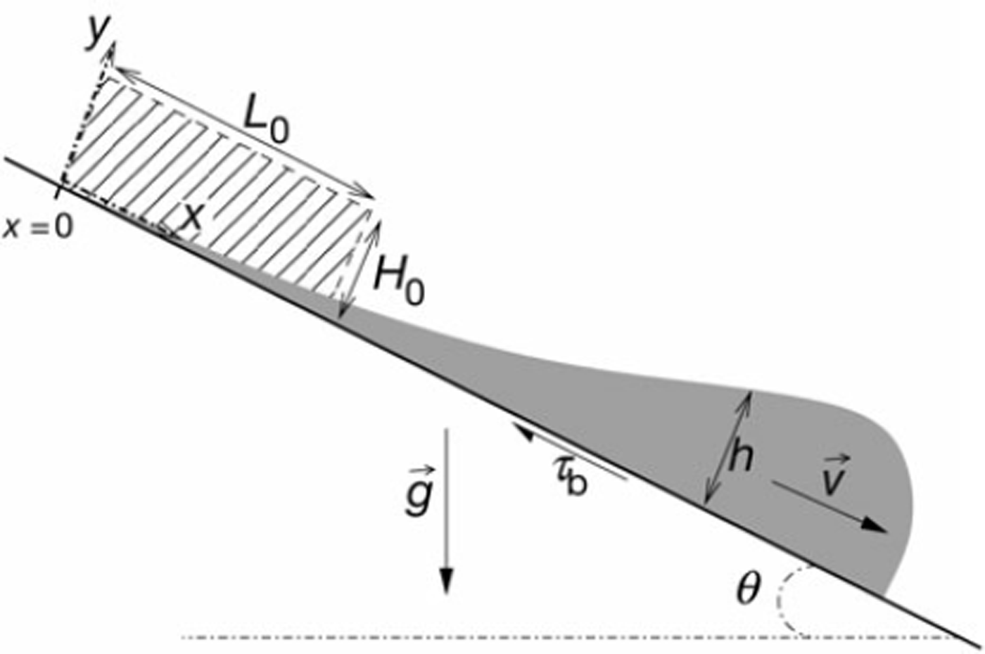
Fig. 1. Schematic representation of the avalanche configuration. The dashed area represents the initial snow mass distribution. The point x = 0 is defined as the upper limit of this initial distribution.
Depth-averaged equations
Within the framework of the assumptions listed above, avalanche propagation can be modelled using the following form of shallow-flow equations (e.g. Reference StokerStoker, 1958):
These two equations constitute the depth-integrated forms of mass and momentum balance, respectively. They govern the coupled evolutions of the flow height, h(x, t), and the downslope, depth-averaged velocity, ![]() . In Equation (2),
. In Equation (2), ![]() denotes gravity acceleration and rb represents the basal shear stress exerted by the bed on the flowing layer (Fig. 1).
denotes gravity acceleration and rb represents the basal shear stress exerted by the bed on the flowing layer (Fig. 1).
The expression for basal shear stress, τ
b, as a function of the variables h and ![]() , accounts for the rheology of the flowing material. To describe dry and dense flowing snow, we use the classical empirical Voellmy law (Reference VoellmyVoellmy, 1955; Reference AnceyAncey, 2006):
, accounts for the rheology of the flowing material. To describe dry and dense flowing snow, we use the classical empirical Voellmy law (Reference VoellmyVoellmy, 1955; Reference AnceyAncey, 2006):
where p0 (dimensionless) and ξ (ms–2) are two frictional coefficients that can be regarded as effective material properties. According to this empirical law, rb is thus expressed as the sum of a Coulomb friction contribution and a hydraulic, Chézy-like resistance term. In the following we will assume that μ 0 < tan 0, in order for steady and uniform flow regimes to exist.
Lastly, as typical in avalanche-propagation models, we also assume that ![]() This amounts to considering the vertical profile of downslope velocity, vx, to be uniform inside the flow. Dropping the bar notation for the depth-averaged velocity
This amounts to considering the vertical profile of downslope velocity, vx, to be uniform inside the flow. Dropping the bar notation for the depth-averaged velocity ![]() , Equations (1) and (2) can then be rewritten as:
, Equations (1) and (2) can then be rewritten as:
These two equations constitute a closed differential system for h and u. They must be supplemented by appropriate boundary conditions; here we impose the condition that velocity goes to zero at the upper end of the initial mass distribution, i.e. at x = 0 (Fig. 1):
This condition models the presence of an ‘impermeable’ wall of static snow. At the opposite end, the height, h, goes to zero at the avalanche front, x = xf(t):
The position of the front, xf(t), is determined by the constant-volume condition:
Numerical solution
The system of Equations (4) and (5) can be solved numerically using what are now relatively standard methods. The first step is to rewrite these equations under the conservative form:
where W = [h, hu], f(W) = [hu, hu2 + gcosθh2/2], and G(W) = [0, gh cosθ(tan θ – μ0) – gcosθu2/ξ]. Besides continuous solutions, this system also admits discontinuous, or shocked, solutions. Across discontinuities, the following Rankine-Hugoniot relationship is verified: [[f(W)]] = σ[[W]], where a is the speed of the discontinuity and [[.]] denotes the difference upstream and downstream of it.
Let us then define a discretization of space and time with dx and dt the corresponding space- and time-steps. Using the notation r = dt/dx and ![]() , a numerical scheme of the form
, a numerical scheme of the form
is consistent with the homogeneous part of Equation (9) if the numerical flux is written as ![]() , where the function F verifies F(W, W) = f(W). Under this condition, Reference LaxLax (1957) and Reference GodunovGodunov (1959) showed that it is possible to build up expressions for the numerical flux such that the resulting schemes (Equation (10)) are stable, robust and properly treat discontinuities. The main drawback of these schemes, however, is their lack of accuracy. To overcome this limitation, several workers (e.g. Reference LerouxLeroux, 1979; Reference Van LeerVan Leer, 1979; Reference LeVequeLeVeque, 2002) improved the accuracy of Godunov-type schemes by adding an anti-diffusion term to the numerical flux. In order to preserve stability in the neighbourhood of discontinuities, this anti-diffusion term has to be limited (min-mod method). For the study presented here, we developed a simplified Godunov solver following such an approach, and adding the contribution of the second-member G(W) to the numerical flux. Several tests have been performed to control the stability, the accuracy and the convergence towards physical solutions of the developed numerical scheme.
, where the function F verifies F(W, W) = f(W). Under this condition, Reference LaxLax (1957) and Reference GodunovGodunov (1959) showed that it is possible to build up expressions for the numerical flux such that the resulting schemes (Equation (10)) are stable, robust and properly treat discontinuities. The main drawback of these schemes, however, is their lack of accuracy. To overcome this limitation, several workers (e.g. Reference LerouxLeroux, 1979; Reference Van LeerVan Leer, 1979; Reference LeVequeLeVeque, 2002) improved the accuracy of Godunov-type schemes by adding an anti-diffusion term to the numerical flux. In order to preserve stability in the neighbourhood of discontinuities, this anti-diffusion term has to be limited (min-mod method). For the study presented here, we developed a simplified Godunov solver following such an approach, and adding the contribution of the second-member G(W) to the numerical flux. Several tests have been performed to control the stability, the accuracy and the convergence towards physical solutions of the developed numerical scheme.
Additionally, appropriate numerical boundary conditions must be prescribed at the ends of the computational domain. To solve the problem of avalanche propagation considered here, we set a reflective boundary condition at x = 0, which corresponds to an impermeable wall (numerical flux equal to zero). The downstream boundary condition was set open by considering null discharge and height gradients. However, this downstream condition is placed sufficiently far away that it is not reached by the flows computed here.
Asymptotic Solution
Kinematic wave approximation
Since we assume that tan 9 > μ0, Equations (4) and (5) admit steady uniform solutions corresponding to a balance between gravity and basal friction. However, for the case of finite-volume releases examined here, fully steady uniform regimes cannot be achieved. It is, nevertheless, reasonable to expect that for sufficiently large times, the dynamics of the avalanche will be governed by this same balance between gravity and friction. Hence, for sufficiently large times, we assume that the momentum balance equation (5) reduces to a simple relationship between velocity and height:
where K = ξ(tan θ – μ0). Note that this relationship is equivalent to stating that the local Froude number, ![]() of the flow is constant both in space and time:
of the flow is constant both in space and time:
Inserting Equation (11) into the mass-balance equation (4) then yields a differential equation for h only, which has the form of a non-linear kinematic wave equation (Reference Lighthill and WhithamLighthill and Whitham, 1955):
To examine the validity of this kinematic wave approximation more precisely, let us establish the conditions under which the inertia and pressure gradient terms on the left-hand side of Equation (5), become negligible compared to gravity and basal friction on the right-hand side. For any given value of time, let H denote the characteristic height and U the characteristic velocity of the avalanche. Inertia terms in Equation (5) are then of the order of U2/xf, while pressure gradient terms are of the order of g cos 9H/xf. A sufficient condition for Equation (5) to reduce to a balance between gravity and friction is thus:
Depending on the parameters 9, μ0 and £, and on the initial values, H0 and L0, condition (14) may or may not be satisfied at early times in the propagation. However, as time proceeds, the front position, xf, will increase and, owing to volume conservation (Hxf ∼ A), the avalanche height, H, will decrease. Hence, regardless of the initial conditions, for the constant-volume and constant-slope case considered here, there necessarily exists a time above which condition (14) will be satisfied. The kinematic wave equation (13) can thus effectively be regarded as an asymptotic approximation of the initial shallow-flow equations (4) and (5) for large times.
Equation (13) being of first order in space, only one boundary condition has now to be specified. According to relationship (11), we note that condition (7) would imply that the front velocity is zero, which is not physically admissible. Hence, in the kinematic wave approximation, the condition of null height at the avalanche front has to be relaxed. As will be shown below, the front is actually represented by a shock (i.e. a height discontinuity) in this approximation. We thus only impose boundary condition (6) which, according to (11), can now be rewritten in terms of flow height:
Self-similar solution
We first rewrite the kinematic wave equation (13) in terms of the following dimensionless variables: ![]() and
and ![]() We obtain:
We obtain:
Similarly, the boundary condition (15) becomes
and the constant-volume condition (8) becomes
We then note that the dimensionless wave equation (16) is invariant under the following stretching groups:
with A > 0 and δ > 0. As a consequence, we can seek solutions presenting identical symmetry properties, that is self-similar solutions of the form (e.g. Reference DresnerDresner, 1999):
with ![]() . Furthermore, assuming also that the similarity variable at the front,
. Furthermore, assuming also that the similarity variable at the front, ![]() , is constant (i.e. looking for a solution in which the front position,
, is constant (i.e. looking for a solution in which the front position, ![]() , is also invariant under transformations (19) and (20)), the value of the exponent 5 is then imposed by the constant-volume condition. Inserting Equation (22) into Equation (18) yields
, is also invariant under transformations (19) and (20)), the value of the exponent 5 is then imposed by the constant-volume condition. Inserting Equation (22) into Equation (18) yields
and thus, if ζ is a constant,
The most interesting property of similarity solutions, such as Equation (22), besides generally being expressible under a closed analytic form, is that, when existing, these solutions constitute the large-time asymptotic form of all other sufficiently regular solutions of the considered differential equation. More precisely, in the case considered here, if a similarity solution of Equation (16) that also satisfies the boundary condition (17) can be found, then all other solutions of Equation (16) satisfying this boundary condition will converge towards this similarity solution at large times, independently of the initial conditions verified by these other solutions (Reference Grundy and RottmanGrundy and Rottmann, 1985; Reference DresnerDresner, 1999). In other words, this similarity solution would represent the general solution of Equation (16) once the influence of the initial conditions has vanished.
Inserting expression (22), with δ = 2/3, into the kinematic wave equation (16), results in an ordinary first-order differential equation for the function P:

Equation (25) can be integrated analytically using the following change of variable: P = ζ2Z2 (Reference Gratton and VigoGratton and Vigo, 1994; Reference Ancey, Cochard, Rentschler and WiederseinerAncey and others, 2007). We obtain an autonomous differential equation for Z:
which readily integrates into:
where CZ ≥ 0 is an integration constant. Accordingly, the original function P is thus given by the following implicit expression:
where the integration constant CP has been redefined in a straightforward manner.
Lastly, the boundary condition (17) becomes, in terms of function P:
This condition implies that CP = 0 in Equation (28). Hence the only solution of Equation (25) which also satisfies boundary condition (29), assumes the following simple form:
This translates into the following expression for the non-dimensional height h:
Properties of the asymptotic solution
Height and velocity profiles
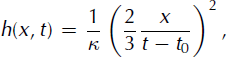
Returning to dimensional quantities, the self-similar solution (31) derived above can be written:

This expression is valid for 0 ≤ x ≤ xf(t). Hence, according to this solution, for any given value of time, t, the height profile of the avalanche has a parabolic shape between x = 0 and the front.
The front position, xf(t), is readily obtained from the constant-volume condition (8):
Accordingly, the front height, h f(t) = h(x f (t), t), can be written:
and also corresponds to the maximum height of the avalanche. We notice that the avalanche front is represented as a height discontinuity (shock) in this self-similar solution (see also Figs 2 and 3).
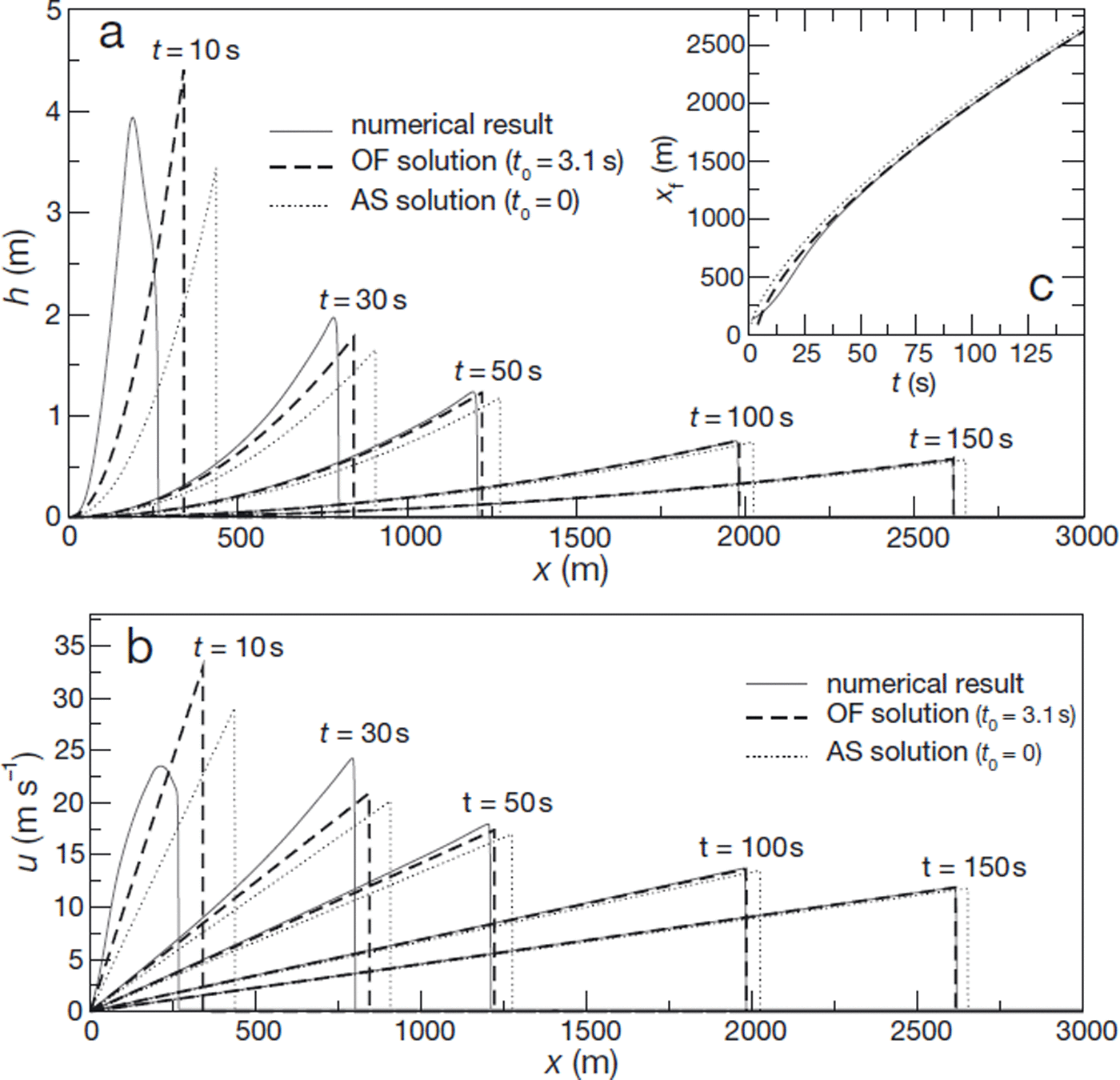
Fig. 2. Comparison between numerical results, asymptotic solution (AS) and offset solution (OF) for simulation s2 (see Table 1). (a) Flow height, h, as a function of abscissa, x, for different values of time. (b) Depth-averaged velocity, u, as a function of abscissa, x, for different values of time. (c) Front position, x f, as a function of time, t.
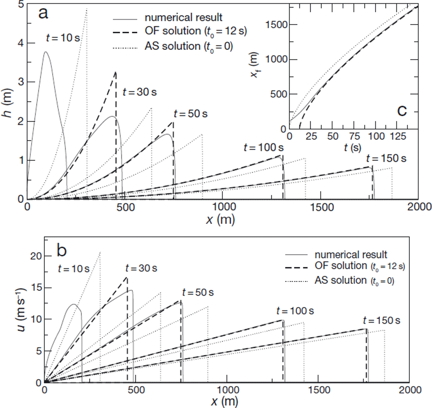
Fig. 3. Comparison between numerical results, asymptotic solution (AS) and offset solution (OF) for simulation s7 (see Table 1). (a) Flow height, h, as a function of abscissa, x, for different values of time. (b) Depth-averaged velocity, u, as a function of abscissa, x, for different values of time. (c) Front position, x f, as a function of time, t.
The velocity profile, u(x, t), derives directly from the height profile (32), through the kinematic wave characteristic relationship (11):
For a given value of t, the velocity profile thus displays a simple linear shape. Lastly, the front velocity, u f, can be expressed as:
It is worth noting that expression (32) was also derived by Reference HuntHunt (1984, Reference Hunt1994) as a solution to the kinematic wave equation (13). He made use of the method of characteristics, postulating an initial condition in which the fluid mass is completely concentrated at point x = 0. The interest of the alternative derivation presented here, based on the notion of self-similarity, is that it demonstrates that this particular solution constitutes the large-time asymptotic form of all the solutions of Equation (13) that verify h(0, t) = 0, regardless of the initial condition. Moreover, as we argued previously, the kinematic wave equation itself constitutes a large-time approximation of the complete shallow-flow equations describing the propagation of constant-volume avalanches. The found solution ((32) and (33)) can thus be considered as representative of the large-time behaviour of all constant-volume avalanches of area A, independently of the particular values of initial height and length, H0 and L0. This solution will hereafter be referred to as the ‘asymptotic solution’.
Lastly, although a trivial consequence of the kinematic wave approximation, it is interesting that, unlike the primitive shallow-flow equations (4) and (5), the derived asymptotic solution depends on slope, 6, and on friction coefficients, μ0 and £, only through the lumped parameter K = ξ(tan θ – μ0). In other words, this means that the asymptotic solution is completely parameterized by the Froude number ![]() (Equation (12)).
(Equation (12)).
Scaling relationships
The most remarkable properties of the found asymptotic solution appear when expressing avalanche height as a function of front position, xf. From Equations (34) and (33), we find the following scaling relationship between front height (or maximum height), hf, and xf:
Similarly, we can define the avalanche average height, (h), with ![]() We easily obtain
We easily obtain
and, thus, the following scaling relationship:
Note that the front position, xf, can also be viewed as the distance travelled by the avalanche since its release. Hence, relationships (37) and (39) imply that, when expressed as a function of the avalanche travel distance, the maximum and average heights of the flow only depend on the avalanche area, A, and are independent of the parameter K (and of the Froude number, Fr). This constitutes a very strong result, meaning that for an observer located at a given distance from the release zone, the height of potential avalanches passing the observer’s position only depends on the volume, and not on the slope, 9, or on the snow friction coefficients, μ 0 and ξ (provided these avalanches match the asymptotic solution).
A similar property is found when looking at avalanche length. Formally, the length of the asymptotic solution is equal to the travel distance, xf, since h > 0 as soon as x > 0. However, flow height becomes vanishingly small as x —> 0. For practical applications, we can thus introduce an avalanche length, Lc, defined with respect to a given height threshold, hc:
where the abscissa, x c(t), is such that h(x c(t),t) = h c. Typically, the threshold, h c, would be of the order of a few snow-grain sizes, a height below which the concept of an avalanche becomes meaningless. After straightforward algebra, we obtain:
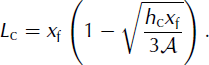
Hence, we observe that when expressed as a function of the travel distance, xf, this measure of avalanche length is also only dependent on the area, A, and is independent of the parameter K.
Numerical Results
Simulation parameters
In order to check the validity of the asymptotic solution and scaling relationships derived in the above section, numerical solutions of the complete shallow-flow equations (4) and (5) have been computed using the numerical scheme described previously. We simulated the propagation of constant-volume avalanches for different values of area, A, in the range 100–1000 m2. These areas correspond to volumes varying between 2000 and 20 000m3 if one assumes, for instance, an avalanche width of 20 m. The desired area values have been achieved by varying both the initial height, H0, and the initial length, L0, of the avalanche (in the range 1–10 m and 50–250 m, respectively), to assess the influence of these two quantities. The snow friction coefficients were held constant in all our simulations: μ 0 = 0.25 and ξ = 750 ms–2 (Reference AnceyAncey, 2006), and two slope values, 9 = 20° and 9 = 30°, were investigated. (Once the kinematic wave approximation is valid, varying the slope is equivalent to varying the friction coefficients, μ 0 and £,, since all are lumped into the single parameter κ. This is not true, however, for the early times of the simulations where inertia terms also play a significant role.)
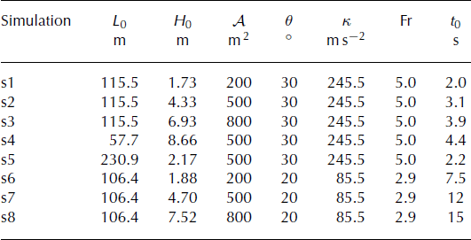
In total, >40 simulations were performed. From these we have selected eight representative simulation results to discuss here. The corresponding parameters are given in Table 1.
Table 1. Parameters of the eight numerical simulations presented here. The quantity t 0 corresponds to the time offset needed to adjust the asymptotic solution to numerical results (see text). It was determined for each simulation by trial and error
Convergence towards asymptotic solution
Time offset
Figures 2 and 3 present direct comparisons between numerical results and the asymptotic solution for the two slope angles. The first important observation is that numerical results do effectively converge towards the predicted solution at large times. However, while the height and velocity profiles rapidly acquire the characteristic shapes (parabolic and linear, respectively) of the self-similar solution, the convergence of the front position towards the predicted value is relatively slow, particularly for θ = 20• (Fig. 3c). This suggests that numerical results would converge much faster towards a slightly modified form of the self-similar solution, in which the time is offset by a constant value, t 0 > 0:
Expressions (42) and (43) define another solution of the kinematic wave equation (13), and also satisfy the boundary and constant-volume conditions of our problem. This new solution will, henceforth, be referred to as the‘offset solution’. As it should, this offset solution converges towards the asymptotic, self-similar solution for t ≫ t0. However, while complete convergence of the simulated avalanches towards the asymptotic solution generally requires several hundreds of seconds, we observe in Figures 2 and 3 that the offset solution, with an appropriate value of t0, constitutes an excellent approximation to the numerical results as soon as t ≥ 50 s, typically. ‘Best-fitting’ values of the time offset, t0, were determined for all our simulations (Table 1).
The only notable discrepancy persisting between numerical results and the best-fitting offset solution concerns the shape of the avalanche front (Figs 2 and 3). The representation of the front as a shock in the theoretical solutions, which is a consequence of the kinematic wave approximation, is relatively crude. In fact, ‘real’ fronts computed numerically with the full shallow-flow equations are steep but not discontinuous. They have a finite length, which appears to progressively decrease as time proceeds, and to be larger for the smallest slope angle. As a consequence, the front height generally tends to be overestimated by the offset solution compared to the numerical results. Note that the existence of smooth, blunted fronts in the simulations is not due to artefactual numerical dissipation, but is representative of the ‘true’ solution of shallow-flow equations. Physically, the kinematic wave approximation ceases to be valid in this region, and should be replaced by a balance between gravity, friction and pressure gradients (Reference WhithamWhitham, 1955; Reference Hogg and PritchardHogg and Pritchard, 2004).
The best-fitting values of the time offset, t 0, appear to be influenced by most simulation parameters, including the initial height of the snow mass, H 0 (Table 1). At first sight, the introduction of this time offset could thus seem to be merely an ad hoc recipe to match the numerical results and the asymptotic solution. Physically, close observation of our results suggests that t 0 probably corresponds to the time needed for the flow height at x = 0 to vanish. However, further work would be needed to fully characterize this parameter. Nevertheless, and regardless of the precise origin of t 0, it is important to remind ourselves that the offset solution presents exactly the same shape and, as a consequence, the same remarkable geometrical properties, as the asymptotic solution. In particular, the scaling relationships (37), (39) and (41) between avalanche height or length and travel distance, remain valid for the offset solution independently of t 0. In that sense, the fact that introducing a time offset is sufficient to render the theoretical large-time solution compatible with numerical results even for ‘intermediate’ times, constitutes an important result: it implies that relationships (37), (39) and (41) are expected to be relevant for real avalanches, even if these avalanches have not fully converged towards the asymptotic solution.
Convergence index
Quantitatively, the convergence between numerical results and the best-fitting offset solution can be characterized using the relationship:
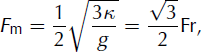
where ![]() is the average Froude number of the avalanche. Straightforward algebra shows that this proportionality between Fm and the local Froude number, Fr, holds for the asymptotic solution as well as for all offset solutions, independently of the value of t0. The coefficient
is the average Froude number of the avalanche. Straightforward algebra shows that this proportionality between Fm and the local Froude number, Fr, holds for the asymptotic solution as well as for all offset solutions, independently of the value of t0. The coefficient ![]() can be regarded as a characteristic of the particular shape of these solutions. We thus define the following convergence index:
can be regarded as a characteristic of the particular shape of these solutions. We thus define the following convergence index:

With the average Froude number, Fm, computed directly from the numerical results, this index characterizes in a single figure the convergence of both height and velocity profiles towards the (best-fitting) offset solution. It tends to zero for full convergence.
As shown in Figure 4, the index, Icv, undergoes a rapid decrease at short times before reaching a slightly negative minimum. It then progressively levels off to the null asymptote. In detail, the minimum value as well as the time needed to reach a given convergence level, depend in a nontrivial manner on all the simulation parameters. However, we note that for all the simulations we conducted (except for the largest area at θ = 20°), the minimum value reached by Icv is above —0.1 (Fig. 4). Hence, convergence levels of 10% or less in terms of Icv are generally reached before the minimum, that is for relatively short times, smaller than 15–25s.
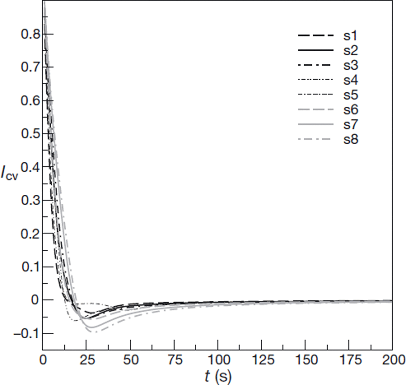
Fig. 4. Convergence index, I cv, as a function of time, t, for the eight simulations.
Similar trends are observed when Icv is plotted as a function of avalanche travel distance, xf, though with an enhanced dispersion between the different curves (Fig. 5a). Interestingly, we also notice that the small-xf evolutions of Icv for the different simulations all appear to collapse on a master curve, at least to a first approximation, when the travel distance, xf, is scaled by ![]() (Fig. 5b). This indicates that convergence towards the offset solution seems to be primarily controlled by a characteristic length equal to
(Fig. 5b). This indicates that convergence towards the offset solution seems to be primarily controlled by a characteristic length equal to ![]() (and not L0 or H0). Typically, as shown in Figure 5b, convergence levels of 10% in terms of index I
cv are reached for travel distances ∼10 to
(and not L0 or H0). Typically, as shown in Figure 5b, convergence levels of 10% in terms of index I
cv are reached for travel distances ∼10 to ![]() .
.
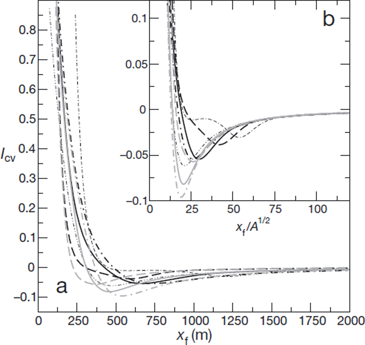
Fig. 5. (a) Convergence index, Icv, as a function of front position (or avalanche travel distance), xf, for the eight simulations. (b) As (a) but with xf normalized by ![]() . The simulations, s1 to s8, are shown in black, red, dashed and dotted, as in Figure 4.
. The simulations, s1 to s8, are shown in black, red, dashed and dotted, as in Figure 4.
Though desirable, a more detailed analysis of the control parameters influencing the evolution of index I cv lies beyond the scope of this study. Work on this is currently in progress. In detail, the convergence of numerical results towards the asymptotic solution is a complex process involving both convergence of the full shallow-flow equations towards the kinematic wave approximation, and convergence of the initial-value solution towards the large-time self-similar solution. Regarding convergence towards the offset solution, the situation is even more complex, due to the presence of the parameter t 0 whose origin, as already mentioned, remains to be precisely established.
Scaling relationships
As shown in Figure 6, numerical results appear to be in excellent agreement with the prediction of scaling relationship (39), concerning the evolution of avalanche average height, (h), as a function of travel distance. When scaled average height, ![]() is plotted against scaled front position,
is plotted against scaled front position, ![]() , the curves corresponding to the different simulations are nearly indistinguishable and fully agree with the theoretical prediction. Moreover, note that good agreement between numerical results and the scaling relationship is found even for small values of xf, i.e. even before full convergence with the offset solution.
, the curves corresponding to the different simulations are nearly indistinguishable and fully agree with the theoretical prediction. Moreover, note that good agreement between numerical results and the scaling relationship is found even for small values of xf, i.e. even before full convergence with the offset solution.
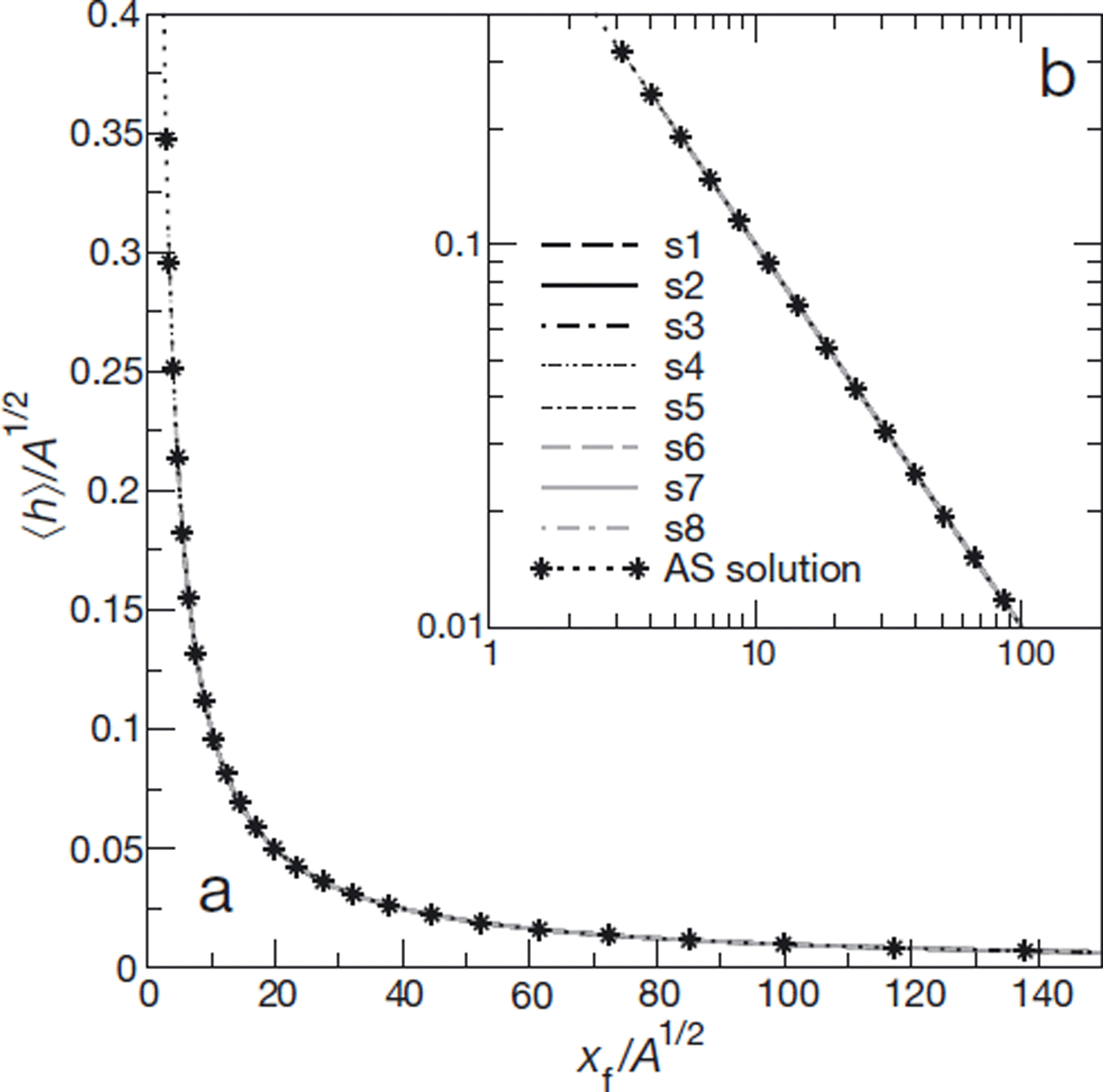
Fig. 6. (a) Scaled average height, ![]() as a function of scaled front position (or avalanche travel distance),
as a function of scaled front position (or avalanche travel distance), ![]() , for the eight simulations, and comparison with scaling relationship (39). (b) As (a), in log-log coordinates.
, for the eight simulations, and comparison with scaling relationship (39). (b) As (a), in log-log coordinates.
The agreement with the theoretical prediction is not as good for the avalanche front height, or maximum height, hf (Fig. 7). Typically, it is only after travel distances ∼40 to ![]() that the scaled curves of
that the scaled curves of ![]() vs
vs ![]() , corresponding to the different simulations, collapse on scaling relationship (37). These travel distances are larger than those required to meet the 10% convergence criterion in terms of I
cv
, corresponding to the different simulations, collapse on scaling relationship (37). These travel distances are larger than those required to meet the 10% convergence criterion in terms of I
cv
![]() . Clearly, this behaviour is due, at least partly, to the over-simplification of the front representation in the kinematic wave approximation.
. Clearly, this behaviour is due, at least partly, to the over-simplification of the front representation in the kinematic wave approximation.
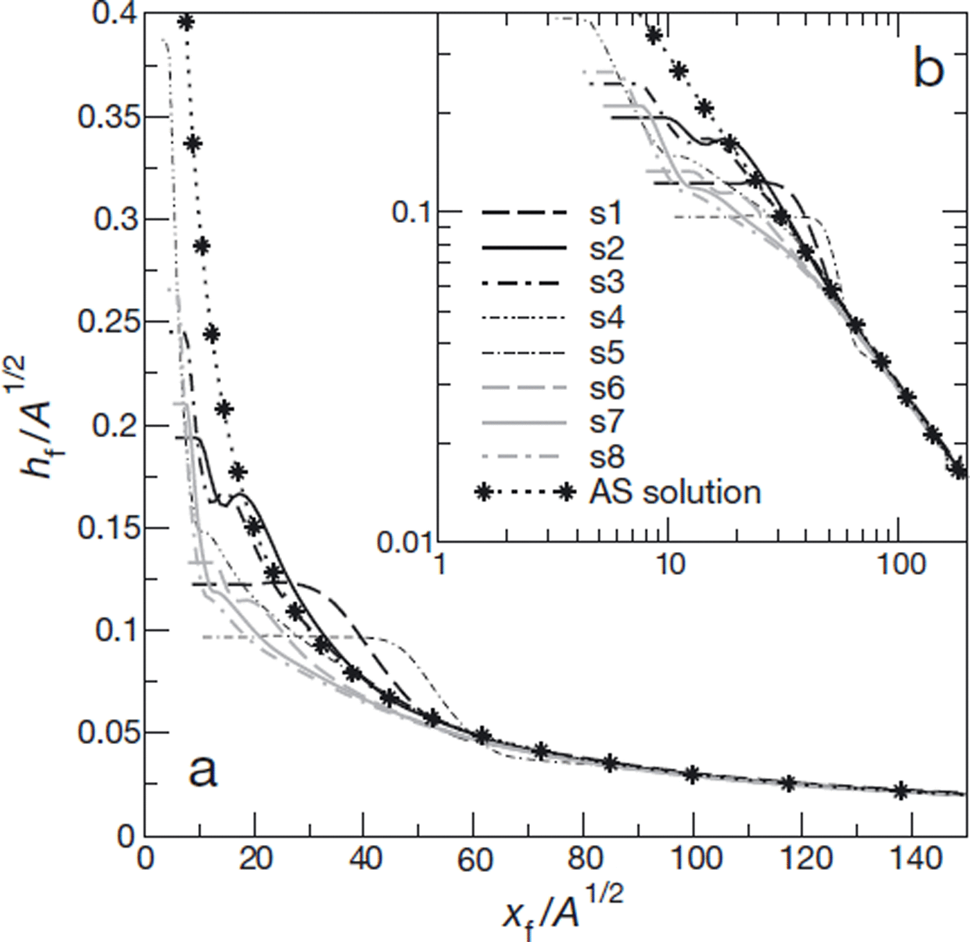
Fig. 7. (a) Scaled front height, ![]() , as a function of scaled front position (or avalanche travel distance),
, as a function of scaled front position (or avalanche travel distance), ![]() , for the eight simulations, and comparison with scaling relationship (37). (b) As (a), in log-log coordinates.
, for the eight simulations, and comparison with scaling relationship (37). (b) As (a), in log-log coordinates.
Finally, results concerning the avalanche length, Lc, are shown in Figure 8. The agreement with the theoretical relationship (41) is excellent, even for small values of travel distance, xf. In particular, we find that Lc
is effectively independent of parameter κ when plotted as a function of xf, but remains dependent on avalanche area, ![]() . Notice also that, with a reasonable value for the height threshold, hc (hc = 0.01 m in Fig. 8), the obtained values of avalanche length, Lc, globally remain very close to the total travel distance, xf. However, as expected, the difference between Lc and xf increases as xf increases.
. Notice also that, with a reasonable value for the height threshold, hc (hc = 0.01 m in Fig. 8), the obtained values of avalanche length, Lc, globally remain very close to the total travel distance, xf. However, as expected, the difference between Lc and xf increases as xf increases.
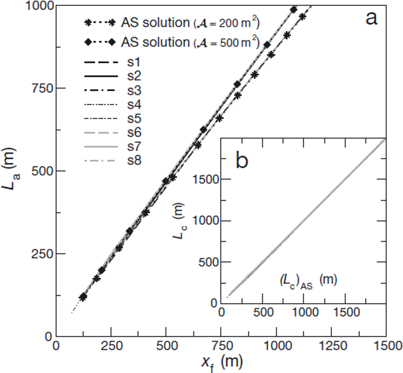
Fig. 8. (a) Avalanche length, L
c, as a function of front position (or avalanche travel distance), x
f, and comparison with relationship (41). For the sake of clarity, only the cases ![]() and 500 m2 are represented. Computations of L
c have been performed on the basis of a height threshold, h
c = 0.01 m. (b) Avalanche length obtained from numerical results as a function of analytic prediction, (L
c)AS, for the eight simulations.
and 500 m2 are represented. Computations of L
c have been performed on the basis of a height threshold, h
c = 0.01 m. (b) Avalanche length obtained from numerical results as a function of analytic prediction, (L
c)AS, for the eight simulations.
Discussion and Conclusions
The results presented in this paper show that, regardless of the initial conditions, the propagation of constant-volume avalanches is rapidly and well captured by a simple approximate solution corresponding to a dynamical balance between gravity and basal friction (the kinematic wave approximation). Although further work is needed to fully characterize the convergence process, for all the performed simulations, good agreement between the numerical results and the approximate solution is observed as soon as the distance travelled by the front is >10 to ![]() , typically. Hence, convergence towards the approximate solution is faster for small-scale than for large-scale avalanches. In general, however, this approximate solution involves an adjustable parameter, namely the time offset, t0, whose value remains dependent on the initial conditions and is difficult to calibrate a priori. For large times, all approximate solutions then tend towards a generic self-similar form independent of t0 and the initial conditions, but this typically occurs for travel distances of
, typically. Hence, convergence towards the approximate solution is faster for small-scale than for large-scale avalanches. In general, however, this approximate solution involves an adjustable parameter, namely the time offset, t0, whose value remains dependent on the initial conditions and is difficult to calibrate a priori. For large times, all approximate solutions then tend towards a generic self-similar form independent of t0 and the initial conditions, but this typically occurs for travel distances of ![]() that are irrelevant for realistic snow avalanches (Figs 2 and 3). Direct use of the approximate solution in practical applications thus appears limited, due to the presence of the time offset, t0.
that are irrelevant for realistic snow avalanches (Figs 2 and 3). Direct use of the approximate solution in practical applications thus appears limited, due to the presence of the time offset, t0.
Importantly, however, some remarkable properties of the approximate solution are independent of t0. In particular, we show that when expressed as a function of the distance travelled by the front, the maximum height, the average height and the length of the avalanche obey simple scaling relationships that are a function only of the avalanche area, ![]() . Numerical results confirm the validity of these scaling relationships. In particular, theoretical predictions for the average height, (h), and for the length, Lc, are in excellent agreement with the simulations, and this even for small travel distances. Concerning the front height, hf, larger travel distances ∼40 to
. Numerical results confirm the validity of these scaling relationships. In particular, theoretical predictions for the average height, (h), and for the length, Lc, are in excellent agreement with the simulations, and this even for small travel distances. Concerning the front height, hf, larger travel distances ∼40 to ![]() are required for full agreement with theoretical predictions. However, note that even in this case, the derived scaling relationship provides a reasonable approximation of hf, typically within 30%, for travel distances
are required for full agreement with theoretical predictions. However, note that even in this case, the derived scaling relationship provides a reasonable approximation of hf, typically within 30%, for travel distances ![]() (Fig. 7).
(Fig. 7).
We thus argue that the obtained scaling relationships (Equations (37), (39) and (41)) can constitute useful tools for experts and engineers. Specifically, these relationships provide simple analytical predictions of the characteristic height and length of avalanches at a given location along the path, with the only required input data being the volume and distance from the release zone. Precise knowledge of the snow friction properties, which can be difficult to assess in practical situations, is not necessary. For instance, it is possible to take advantage of these scaling relationships to directly compare the characteristic dimensions of two different avalanches released in the same zone, but of different areas (or volumes per unit width), ![]() and
and ![]() . From (37) and (39) we obtain:
. From (37) and (39) we obtain:
An analogous, though more complex, expression can be derived from Equation (41) for the ratio of lengths, Lc. Of course, in practical applications, the exact figures derived from these scaling relationships need to be treated with caution, due to the various hypotheses involved in their derivation (see below). However, their use can represent a valuable first approach, allowing reasonable orders of magnitude to be obtained rapidly and easily, prior to employing more sophisticated models. An example of the application of relationship (46) for the design of a protection structure, is presented by Reference Naaim, Faug, Naaim and EckertNaaim and others (2010).
Among the hypotheses involved in the derivation of the asymptotic solution presented in this paper, two may appear particularly restrictive; namely, the constant slope and the constant volume. To investigate the influence of the constant-slope assumption, we performed preliminary numerical simulations involving an abrupt slope reduction in the avalanche path (Fig. 9), leaving the other simulation parameters the same as for the constant-slope simulations. We observe that once the front has passed the slope break, the avalanche body can be viewed as constituted of two distinct parts, one on the high-slope zone and one on the low-slope zone, with mass progressively transiting from the upstream to the downstream part. Interestingly, the flow height in each of these two parts exhibits the characteristic parabolic shape of the self-similar solution, and could be well represented by variants of Equation (32) with varying areas and proper time and space offsets. The transition zone between the two parabolic branches is relatively narrow. This preliminary result suggests that the approximate solution and the scaling relationships presented in this paper, could probably be generalized, with only minor refinements, to situations of variable slope (at least in the, not infrequent, cases where the avalanche path can be described as a succession of constant-slope sections). Such developments are currently in progress.
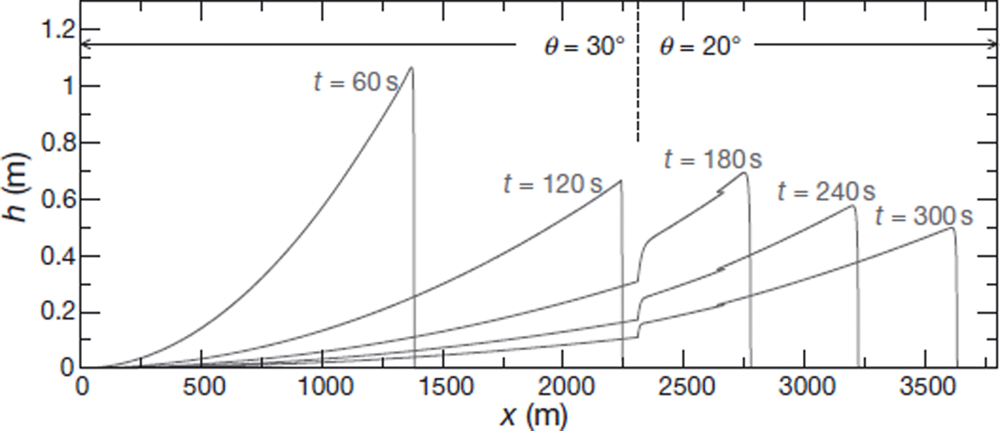
Fig. 9. Numerical simulation of an avalanche propagating over an abrupt slope break in its bed located at x = 2300 m (6 = 30° upstream, 0 = 20° downstream): flow height, h, as a function of abscissa, x, for different values of time. Initial height and length of the snow mass were, respectively, taken as H0 = 4.33 m and L0 = 115.5 m, thus ![]() . Values of snow friction coefficients are, as previously, JJ,0 = 0.25 and ξ = 750 m s–2.
. Values of snow friction coefficients are, as previously, JJ,0 = 0.25 and ξ = 750 m s–2.
The assumption of constant volume appears to be more restrictive. As a first approximation, this assumption is interesting, allowing us to identify characteristic behaviours that are due solely to avalanche dynamics and rheology. However, it is well known that, depending on flow characteristics and snow properties, snow erosion and deposition processes may induce significant variations of avalanche volume along the propagation and, as a consequence, may also strongly influence avalanche dynamics (Reference Naaim, Faug and Naaim-BouvetNaaim and others, 2003; Reference Sovilla, Burlando and BarteltSovilla and others, 2006). Hence, the results presented in this paper should be regarded as relevant essentially for relatively small-scale avalanches, for which erosion and deposition phenomena remain limited, and probably not for very large catastrophic events. Our results might also hold for mature, even possibly large, avalanches in which the erosion and deposition fluxes globally compensate. From a more general perspective, no evident generalization of the analytic solution derived in this paper (Equation (32)) is expected for the case of variable-volume avalanches. Nevertheless, shallow-flow equations have been shown to admit self-similar solutions in a wide variety of problems, including gravity currents with variable influx (Reference Gratton and VigoGratton and Vigo, 1994; Reference Ancey, Cochard, Rentschler and WiederseinerAncey and others, 2007). It is thus likely that, for some particular forms of erosion and deposition fluxes, the large-time behaviour of variable-volume avalanches can also be described by specific self-similar solutions. Here again, further work is needed.
Finally, we note that a relatively straightforward improvement to our model would be to refine the front description by dropping the kinematic wave approximation in this zone. This would lead to matching an ‘inner’ solution governed by a balance between gravity, friction and pressure gradients, valid only in the front zone, to the ‘outer’ self-similar solution derived above, which is valid in the whole body (Reference WhithamWhitham, 1955; Reference HuntHunt, 1984). Such a refinement would allow the blunted fronts observed in the numerical simulations to be accounted for, and would certainly reduce the travel distance required to obtain good agreement between theoretical predictions and numerical results concerning the front height (Fig. 7). This, however, would be at the expense of simplicity, and the resulting relationship between front height and travel distance would lose one of the main features of Equation (37) – its independence of slope and friction parameters.
Acknowledgements
Financial support from the French National Agency for Research (ANR-MONHA) is gratefully acknowledged. The authors thank an anonymous reviewer for his thoughtful comments.


