


1 Introduction
A dusty plasma is a four-component plasma system consisting of ions, electrons, neutral particles and charged microparticles (i.e. the dust). In the laboratory setting, the dust component consists of nanometre- to micrometre-sized particles. This large size, coupled with the high charge state (typically hundreds to thousands of fundamental units of charge), results in the dust having a relatively low charge to mass ratio and characteristic frequencies of the order of hertz. As a result, it is possible to study the dust component at the particle (i.e. kinetic) level by observing the motion of individual dust grains though the use of video imaging. In the typical dusty plasma experiment, this is accomplished by positioning a camera perpendicular to a laser sheet that illuminates a thin sheet of the dust particles that are suspended in the plasma. It is then possible to measure the motion of the dust grains in the acquired images. From these measurements of particle transport, it is then possible to gain insight into the underlying physics that governs the behaviour of the dust component, as well as the state of the background plasma. For systems with sufficiently low number densities, particle tracking velocimetry (PTV) techniques are often employed to measure the motion of individual dust grains (Feng, Goree & Liu Reference Feng, Goree and Liu2007; Ticos et al. Reference Ticos, Toader, Munteanu, Banu and Scurtu2013; Melzer et al. Reference Melzer, Himpel, Killer and Mulsow2016). For dusty plasmas with higher number densities, where it is difficult to identify or track individual particles, particle image velocimetry (PIV) techniques can be used to measure the motion of groups of particles (Thomas Jr Reference Thomas1999; Thomas Jr, Williams & Silver Reference Thomas, Williams and Silver2004; Williams Reference Williams2011; Williams et al. Reference Williams, Thomas, Couëdel, Ivlev, Zhdanov, Nosenko, Thomas and Morfill2012). Figure 1 illustrates the representative number densities that are typically present when using these different techniques.
This manuscript will provide an overview of the PIV technique, with a specific focus on its application to dusty plasmas. Section 2 will provide an overview of the PIV technique and the variations of this technique that have been employed in the study of dusty plasmas, examine the physical properties that can be measured using these techniques and highlight the parameter regime where this technique is most appropriate. Section 3 will present a small selection of measurements that have been made using this technique, while § 4 will present potential future directions for this diagnostic technique in its application to dusty plasmas.

Figure 1. Images showing representative number densities that typically present when using the (a) PTV and (b) PIV techniques.
2 PIV
PIV is a fluid measurement technique that measures the average motion of a group of particles by comparing a pair of images that are separated in time by a known interval
 ${\rm\Delta}t_{PIV}$
. In this approach, a pair of laser pulses are aligned to follow the same optical path and expanded into a sheet of light that illuminates a region of the experimental system (i.e. the dust cloud). The light that is scattered from the dust grains is imaged by (typically CCD) camera(s) that are synchronized to the laser pulses, acquiring pairs of images for analysis. The synchronization of the cameras and laser pulses, as well as the timing between the laser pulses, are critical in the acquisition of data and are achieved through the use of programmable timing units. Figure 2 illustrates the typical orientation of the laser and cameras used in the various dedicated PIV systems that have been used in the study of dusty plasmas. A spatial correlation analysis is then performed on the acquired images, providing a rapid reconstruction of the particle displacements over the illuminated region of the experimental system in the field of view of the camera(s) with good spatial resolution (
${\rm\Delta}t_{PIV}$
. In this approach, a pair of laser pulses are aligned to follow the same optical path and expanded into a sheet of light that illuminates a region of the experimental system (i.e. the dust cloud). The light that is scattered from the dust grains is imaged by (typically CCD) camera(s) that are synchronized to the laser pulses, acquiring pairs of images for analysis. The synchronization of the cameras and laser pulses, as well as the timing between the laser pulses, are critical in the acquisition of data and are achieved through the use of programmable timing units. Figure 2 illustrates the typical orientation of the laser and cameras used in the various dedicated PIV systems that have been used in the study of dusty plasmas. A spatial correlation analysis is then performed on the acquired images, providing a rapid reconstruction of the particle displacements over the illuminated region of the experimental system in the field of view of the camera(s) with good spatial resolution (
 ${\sim}1~\text{mm}$
) and sub-pixel accuracy (as small as 0.1 pixel, depending on the quality of the image data). The velocity is then found by dividing the measured displacement by the time between the acquired images,
${\sim}1~\text{mm}$
) and sub-pixel accuracy (as small as 0.1 pixel, depending on the quality of the image data). The velocity is then found by dividing the measured displacement by the time between the acquired images,
 ${\rm\Delta}t_{PIV}$
. It is noted that the vector quality can be improved by completing some image processing prior to performing this correlation analysis to reduce image noise (i.e. light from the background plasma glow) and remove non-uniformities in the image intensity. While it is possible to apply the PIV analysis technique to data where particle tracking can be used, the PIV technique is most appropriate for systems with higher number densities and can provide an accurate measurement of the particle transport in cases where the particle densities exceed those where particle tracking techniques can be used. It is particularly effective at identifying fluid behaviour provided that there is not a significant amount of shear in the observed particle motion. For more details on the PIV technique, the reader is referred to several excellent review articles and manuscripts (Westerweel Reference Westerweel1997; Prasad Reference Prasad2000a
,Reference Prasad
b
; Elsinga et al.
Reference Elsinga, Scarano, Wieneke and van Oudheusden2006; Raffel et al.
Reference Raffel, Willert, Wereley and Kompenhans2007; Brossard et al.
Reference Brossard, Monnier, Barricau and Vandernoot2009; Scarano Reference Scarano2013).
${\rm\Delta}t_{PIV}$
. It is noted that the vector quality can be improved by completing some image processing prior to performing this correlation analysis to reduce image noise (i.e. light from the background plasma glow) and remove non-uniformities in the image intensity. While it is possible to apply the PIV analysis technique to data where particle tracking can be used, the PIV technique is most appropriate for systems with higher number densities and can provide an accurate measurement of the particle transport in cases where the particle densities exceed those where particle tracking techniques can be used. It is particularly effective at identifying fluid behaviour provided that there is not a significant amount of shear in the observed particle motion. For more details on the PIV technique, the reader is referred to several excellent review articles and manuscripts (Westerweel Reference Westerweel1997; Prasad Reference Prasad2000a
,Reference Prasad
b
; Elsinga et al.
Reference Elsinga, Scarano, Wieneke and van Oudheusden2006; Raffel et al.
Reference Raffel, Willert, Wereley and Kompenhans2007; Brossard et al.
Reference Brossard, Monnier, Barricau and Vandernoot2009; Scarano Reference Scarano2013).
Within the dusty plasmas community, the majority of measurements that have employed PIV techniques have been made using dedicated PIV systems, where a region of the dust cloud is illuminated by a light sheet created by expanding the output of a pair of pulsed lasers,
 ${\rm\Delta}t_{laser}\sim$
tens of nanoseconds. The shortness of the illumination time ensures that the particles do not move while the image is being acquired, which is important when applying the PIV analysis technique. The camera(s) are synchronized to the firing of pulsed lasers and the experimentalist determines the time between the acquired images, typically
${\rm\Delta}t_{laser}\sim$
tens of nanoseconds. The shortness of the illumination time ensures that the particles do not move while the image is being acquired, which is important when applying the PIV analysis technique. The camera(s) are synchronized to the firing of pulsed lasers and the experimentalist determines the time between the acquired images, typically
 $0.4~{\rm\mu}\text{s}\leqslant t_{PIV}\leqslant 30~\text{ms}$
, before the measurement is made. The value of
$0.4~{\rm\mu}\text{s}\leqslant t_{PIV}\leqslant 30~\text{ms}$
, before the measurement is made. The value of
 ${\rm\Delta}t_{PIV}$
that is used determines the type of motion that can be examined (i.e. kinetic motion with small values of
${\rm\Delta}t_{PIV}$
that is used determines the type of motion that can be examined (i.e. kinetic motion with small values of
 ${\rm\Delta}t_{PIV}$
, fluid motion with larger values of
${\rm\Delta}t_{PIV}$
, fluid motion with larger values of
 ${\rm\Delta}t_{PIV}$
or a combination of kinetic and fluid motion with intermediate values of
${\rm\Delta}t_{PIV}$
or a combination of kinetic and fluid motion with intermediate values of
 ${\rm\Delta}t_{PIV}$
) (Thomas Jr & Williams Reference Thomas and Williams2006). To date, three increasingly sophisticated PIV techniques have been used in the study of dusty plasmas: planar PIV (Thomas Jr Reference Thomas1999), stereoscopic PIV (Thomas Jr et al.
Reference Thomas, Williams and Silver2004) and tomographic PIV (Williams Reference Williams2011). Images depicting the experimental set-ups used in these different iterations of the PIV technique can be seen in figure 2(b–d) and details on the application of these dedicated systems can be found in §§ 2.1–2.3.
${\rm\Delta}t_{PIV}$
) (Thomas Jr & Williams Reference Thomas and Williams2006). To date, three increasingly sophisticated PIV techniques have been used in the study of dusty plasmas: planar PIV (Thomas Jr Reference Thomas1999), stereoscopic PIV (Thomas Jr et al.
Reference Thomas, Williams and Silver2004) and tomographic PIV (Williams Reference Williams2011). Images depicting the experimental set-ups used in these different iterations of the PIV technique can be seen in figure 2(b–d) and details on the application of these dedicated systems can be found in §§ 2.1–2.3.

Figure 2. (a) Cartoon depicting the typical camera orientations that can be used when applying the PIV technique. In the study of dusty plasmas, cameras are typically positioned perpendicular, P, to the illuminated region of the dust cloud (green rectangle). The forward, F, and back, B, scattering positions are preferable when applying stereoscopic and tomographic PIV due to the higher scattering efficiencies. The orientation (left) and images (right) depicting the physical set-up of the (b) planar and (c) stereoscopic PIV systems at Auburn University and the (d) tomographic PIV system at Wittenberg University are seen to the right. (Photos in (b) and (c) courtesy of E. Thomas, Jr., Auburn University, AL.)
While dedicated PIV systems are optimized for the PIV analysis technique, it is not necessary that one use a dedicated system. Indeed, the PIV analysis technique can be applied to any sequence of images, provided that the particles generally do not move in any significant way while the individual images are acquired (i.e. the particles in the acquired image appear point-like and particle streaking is minimal), the time between the acquired images is well known and there is not a significant variation in the particle intensity over the acquired image (Nobach & Bodenschatz Reference Nobach and Bodenschatz2009). As a result, it is possible to apply the PIV analysis technique to images that have been acquired using traditional dusty plasma imaging systems where a single camera is positioned perpendicular to a light sheet that is generated by expanding the output of a continuous wave (CW) laser. In this approach, the frame rate and exposure time of the camera determine when the images are acquired and the user can then select the image pair to use in the PIV analysis once the data have been acquired. Here, the exposure time, which acts as
 ${\rm\Delta}t_{laser}$
, must be short enough to yield images of sufficient quality and the time between the images used in applying the PIV analysis functions as
${\rm\Delta}t_{laser}$
, must be short enough to yield images of sufficient quality and the time between the images used in applying the PIV analysis functions as
 ${\rm\Delta}t_{PIV}$
. It is noted that in this approach, the value of
${\rm\Delta}t_{PIV}$
. It is noted that in this approach, the value of
 ${\rm\Delta}t_{PIV}$
does not need to be determined a priori, allowing the researcher to select the type of motion (i.e. particle motion, fluid motion or a combination) that they are interested in observing after the data has been acquired. This represents a significant advance in the application of this analysis technique compared to its use on dedicated systems where these decisions must be made a priori. Additionally, the recent introduction of higher frame-rate cameras (frame rates
${\rm\Delta}t_{PIV}$
does not need to be determined a priori, allowing the researcher to select the type of motion (i.e. particle motion, fluid motion or a combination) that they are interested in observing after the data has been acquired. This represents a significant advance in the application of this analysis technique compared to its use on dedicated systems where these decisions must be made a priori. Additionally, the recent introduction of higher frame-rate cameras (frame rates
 ${>}50~\text{fps}$
) allows for significantly higher temporal resolution than is possible with the dedicated PIV systems currently used. This approach, referred to as time-resolved PIV, (Williams et al.
Reference Williams, Thomas, Couëdel, Ivlev, Zhdanov, Nosenko, Thomas and Morfill2012) has been used in recent years by a number of groups within the dusty plasma community (Boessé et al.
Reference Boessé, Henry, Hyde and Matthews2004; Arp et al.
Reference Arp, Block, Klindworth and Piel2005; Pilch, Reichstein & Piel Reference Pilch, Reichstein and Piel2008; Kaur et al.
Reference Kaur, Bose, Chattopadhyay, Sharma, Ghosh, Saxena and Thomas2015b
; Chai & Bellan Reference Chai and Bellan2016) and is discussed in § 2.4.
${>}50~\text{fps}$
) allows for significantly higher temporal resolution than is possible with the dedicated PIV systems currently used. This approach, referred to as time-resolved PIV, (Williams et al.
Reference Williams, Thomas, Couëdel, Ivlev, Zhdanov, Nosenko, Thomas and Morfill2012) has been used in recent years by a number of groups within the dusty plasma community (Boessé et al.
Reference Boessé, Henry, Hyde and Matthews2004; Arp et al.
Reference Arp, Block, Klindworth and Piel2005; Pilch, Reichstein & Piel Reference Pilch, Reichstein and Piel2008; Kaur et al.
Reference Kaur, Bose, Chattopadhyay, Sharma, Ghosh, Saxena and Thomas2015b
; Chai & Bellan Reference Chai and Bellan2016) and is discussed in § 2.4.
2.1 Planar PIV
Planar PIV (figure 2
b) was first used in the study of dusty plasmas in 1999 (Thomas Jr Reference Thomas1999). In this approach, a pair of images are acquired by a single camera that is oriented perpendicular to, and synchronized with, a pair of laser pulses that follow the same optical path and are expanded into a light sheet to illuminate a thin slice of the dust cloud. Each image pair (figure 3
a) is then divided into
 $n\times n$
subregions known as interrogation regions (figure 3
b) and a cross-correlation analysis, (2.1), is performed using similar subregions from the image pair (Keane & Adrian Reference Keane and Adrian1990, Reference Keane and Adrian1992). Overlapping interrogation regions are often employed to improve the spatial resolution and the quality of the measured displacements
$n\times n$
subregions known as interrogation regions (figure 3
b) and a cross-correlation analysis, (2.1), is performed using similar subregions from the image pair (Keane & Adrian Reference Keane and Adrian1990, Reference Keane and Adrian1992). Overlapping interrogation regions are often employed to improve the spatial resolution and the quality of the measured displacements
 $$\begin{eqnarray}\displaystyle R(m,n) & = & \displaystyle R_{D}(m,n)+R_{F}(m,n)+R_{C}(m,n)\nonumber\\ \displaystyle & = & \displaystyle \mathop{\sum }_{i,j}I(i,j,t_{1})I(i+m,j+n,t_{2}),\end{eqnarray}$$
where
 $R(m,n)$
is an element in the correlation plane,
$R(m,n)$
is an element in the correlation plane,
 $R_{D}(m,n)$
,
$R_{D}(m,n)$
,
 $R_{F}(m,n)$
and
$R_{F}(m,n)$
and
 $R_{C}(m,n)$
represents that correlation between identical particles, the correlation between random particles and the convolution of background image intensity at location
$R_{C}(m,n)$
represents that correlation between identical particles, the correlation between random particles and the convolution of background image intensity at location
 $(m,n)$
in the correlation plane, respectively and
$(m,n)$
in the correlation plane, respectively and
 $I(i,j,t_{k})$
represents the image intensity at pixel location
$I(i,j,t_{k})$
represents the image intensity at pixel location
 $(i,j)$
in the interrogation region at time
$(i,j)$
in the interrogation region at time
 $t_{k}$
,
$t_{k}$
,
 $k=1,2$
. While several algorithms have been developed to perform this correlation analysis (Meinhart, Wereley & Santiago Reference Meinhart, Wereley and Santiago2000; Piirto et al.
Reference Piirto, Eloranta, Saarenrinne and Karvinen2005; Sciacchitano, Scarano & Wieneke Reference Sciacchitano, Scarano and Wieneke2012), the most common algorithm currently employed within the dusty plasma community is the standard fast Fourier transform cross-correlation function, as described in sections 3.4 and 5.4 of Raffel et al. (Reference Raffel, Willert, Wereley and Kompenhans2007).
$k=1,2$
. While several algorithms have been developed to perform this correlation analysis (Meinhart, Wereley & Santiago Reference Meinhart, Wereley and Santiago2000; Piirto et al.
Reference Piirto, Eloranta, Saarenrinne and Karvinen2005; Sciacchitano, Scarano & Wieneke Reference Sciacchitano, Scarano and Wieneke2012), the most common algorithm currently employed within the dusty plasma community is the standard fast Fourier transform cross-correlation function, as described in sections 3.4 and 5.4 of Raffel et al. (Reference Raffel, Willert, Wereley and Kompenhans2007).

Figure 3. (a) Representative image of a dust cloud with a
 $32\times 32$
pixel grid superimposed. (b) Representative interrogation regions showing a small fraction of the dust grains visible from the blue box seen in (a) and separated in time by
$32\times 32$
pixel grid superimposed. (b) Representative interrogation regions showing a small fraction of the dust grains visible from the blue box seen in (a) and separated in time by
 ${\rm\Delta}t_{PIV}=t_{2}-t_{1}$
. (c) The correlation map that is constructed by performing the PIV analysis on the interrogation regions seen in (b). The resulting correlation map consists of three parts, the correlation between identical particles,
${\rm\Delta}t_{PIV}=t_{2}-t_{1}$
. (c) The correlation map that is constructed by performing the PIV analysis on the interrogation regions seen in (b). The resulting correlation map consists of three parts, the correlation between identical particles,
 $R_{D}$
, the correlation between random particles,
$R_{D}$
, the correlation between random particles,
 $R_{F}$
, and the convolution of background image intensity,
$R_{F}$
, and the convolution of background image intensity,
 $R_{C}$
. Here, the average displacement is represented by the peak denoted by
$R_{C}$
. Here, the average displacement is represented by the peak denoted by
 $R_{D}$
, while
$R_{D}$
, while
 $R_{F}+R_{C}$
represents the noise in the measurement.
$R_{F}+R_{C}$
represents the noise in the measurement.
The resulting correlation plane (figure 3 c) represents a statistical measurement of the particle displacement and the peak in the correlation plane represents the most likely displacement of the particles located in the interrogation region (figure 3 b). This peak is then fit to find the average displacement of the particles in the interrogation region that was used in the application of the PIV algorithm. This fitting yields an uncertainty in the measured displacement that can be as small as 0.1 pixel. This process is repeated over the entire image, yielding an instantaneous measurement of the particle transport over the field of view of the camera. Often, this correlation analysis is repeated several times using the velocity field from the previous iteration to offset and deform the interrogation region used in the subsequent correlation analysis (Kim & Sung Reference Kim and Sung2006). This leads to fewer particles leaving the interrogation regions that are used in the final iteration (Kim & Sung Reference Kim and Sung2006) and a more accurate measurement of the particle displacement (Scarano & Riethmuller Reference Scarano and Riethmuller2000; Scarano Reference Scarano2002).
Because the correlation analysis is essentially a statistical particle-matching technique, it is important that there be several particles in each interrogation region. Additionally, the size of the interrogation region that is used depends on the value of
 ${\rm\Delta}t_{PIV}$
used when acquiring the data. In particular, there are three factors that should be met for the PIV algorithm to accurately capture the particle motion: the particles in each interrogation region should exhibit directed motion (i.e. the majority of the particles in an interrogation region should move in the same direction), the typical displacement of the particles in the interrogation region should be of the order of or less than
${\rm\Delta}t_{PIV}$
used when acquiring the data. In particular, there are three factors that should be met for the PIV algorithm to accurately capture the particle motion: the particles in each interrogation region should exhibit directed motion (i.e. the majority of the particles in an interrogation region should move in the same direction), the typical displacement of the particles in the interrogation region should be of the order of or less than
 $1/4$
the size of the interrogation region used in the PIV analysis and a minimal number of particles should leave the interrogation region over the duration of the measurement,
$1/4$
the size of the interrogation region used in the PIV analysis and a minimal number of particles should leave the interrogation region over the duration of the measurement,
 ${\rm\Delta}t_{PIV}$
. Recent advances in PIV algorithms, including the use of non-square interrogation and search regions, allow for larger displacements to be measured. However, it is critical that directed motion be observed at the scale size of the interrogation region selected.
${\rm\Delta}t_{PIV}$
. Recent advances in PIV algorithms, including the use of non-square interrogation and search regions, allow for larger displacements to be measured. However, it is critical that directed motion be observed at the scale size of the interrogation region selected.
While the planar technique has proven to be a valuable diagnostic tool and has provided significant insight into a range of phenomena including particle transport (Thomas Jr Reference Thomas1999, Reference Thomas2001a , Reference Thomas2002b ; Thomas Jr et al. Reference Thomas, Amatucci, Compton and Christy2002a ; Aldewereld & Thomas Jr Reference Aldewereld and Thomas2007) the potential structure within a dust cloud (Thomas Jr Reference Thomas2002a ) and near the dust-cloud boundary (Thomas Jr Reference Thomas2001b ; Thomas Jr et al. Reference Thomas, Annaratone, Morfill and Rothermel2002b ; Thomas Jr Reference Thomas2003) and the structure of the dust acoustic wave, (Thomas Jr & Merlino Reference Thomas and Merlino2001), one important limitation is that this technique only measures the projection of the motion of the dust grains seen by the cameras onto the plane of the laser sheet. As a result, the motion perpendicular to the laser sheet is lost. While this is not a significant issue for two-dimensional dusty plasma systems, this can be significant for many of the three-dimensional dusty plasma systems which are often in a weakly coupled state and exhibit transport that is fully three-dimensional. For these systems, this projection of the observed motion onto the illuminated slice of the dust cloud represents a limitation of this technique, particularly when looking at the dust cloud–plasma boundary, wave structure or systems where there is significant motion in the direction perpendicular to the laser sheet that is used to illuminate the dust cloud (Thomas Jr et al. Reference Thomas, Williams and Silver2004).
2.2 Stereoscopic PIV
Stereoscopic PIV (figure 2
c) (Prasad Reference Prasad2000b
) was first used in the study of dusty plasmas in 2004 (Thomas Jr et al.
Reference Thomas, Williams and Silver2004) and is an extension of the planar PIV technique. Here, two cameras are oriented obliquely to the plane of the laser sheet and each camera records a pair of images that are synchronized to the firing of a pair of lasers. The oblique viewing angles between each camera and the laser sheet results in non-uniform magnification across the field of view and the images being distorted (Prasad & Jensen Reference Prasad and Jensen1995). To account for this distortion, each camera is fitted with a tilt adapter between the camera lens and the imaging sensor. The field of view of each camera is adjusted using this tilt adapter until no distortion is observed and an empirical calibration is performed to determine a calibration function that describes the orientation of each camera relative to the laser sheet (Tsai Reference Tsai1986). Once the calibration process is complete, a PIV measurement can be made and a pair of two-dimensional velocity fields are computed using the image pairs acquired by each camera. The resulting pair of velocity fields that are generated represent the projection of the particle motion onto the illumination plane measured by each of the cameras. The true three-component velocity vector (
 $v_{x},v_{y},v_{z}$
) of a cluster of particles in a sub-region of the acquired images is reconstructed from this pair of two-dimensional velocity fields and the empirical calibration function.
$v_{x},v_{y},v_{z}$
) of a cluster of particles in a sub-region of the acquired images is reconstructed from this pair of two-dimensional velocity fields and the empirical calibration function.
This technique has provided significant insight into a range of phenomena involving the strength of the neutral drag force (Thomas Jr & Williams Reference Thomas and Williams2005), the spatial structure and thermal properties of the dust acoustic wave (Thomas Jr Reference Thomas2006, Reference Thomas2010; Fisher & Thomas Jr Reference Fisher and Thomas2010) and the thermal state of weakly coupled dusty plasma systems (Williams & Thomas Jr Reference Williams and Thomas2007; Fisher & Thomas Jr Reference Fisher and Thomas2011, Reference Fisher and Thomas2012, Reference Fisher and Thomas2013; Fisher et al.
Reference Fisher, Avinash, Thomas, Merlino and Gupta2013). However, these measurements of the three-dimensional transport are restricted to a thin slice of the dusty plasma system and may not fully capture the true three-dimensional motion if particles leave the laser sheet during the duration of the measurement,
 ${\rm\Delta}t_{PIV}$
. Additionally, the reconstruction of the third velocity component requires spatial calibrations that are accurate to within a few pixels. As a result, these systems, when compared to the planar PIV systems, are much more sensitive to mechanical noise. It is noted, however, that is possible to use the image data acquired during an experiment to correct the mapping function, thereby accounting for small changes that might have occurred between the calibration process and the acquisition of data; including small errors in the initial calibration function or minor shifts in the relative orientation of the cameras and laser sheet due to mechanical vibrations. This self-calibration technique (Wieneke Reference Wieneke2005) identifies a small subset of particles in each of the acquired images and their triangulation in three-dimensional space over the measurement sequence to determine a statistical estimate of the local disparity vector that represents the most probable offset between the lines of sight for the different cameras and the laser sheet. This disparity vector can then be used to correct the calibration function, essentially eliminating this as a concern when using the stereoscopic approach.
${\rm\Delta}t_{PIV}$
. Additionally, the reconstruction of the third velocity component requires spatial calibrations that are accurate to within a few pixels. As a result, these systems, when compared to the planar PIV systems, are much more sensitive to mechanical noise. It is noted, however, that is possible to use the image data acquired during an experiment to correct the mapping function, thereby accounting for small changes that might have occurred between the calibration process and the acquisition of data; including small errors in the initial calibration function or minor shifts in the relative orientation of the cameras and laser sheet due to mechanical vibrations. This self-calibration technique (Wieneke Reference Wieneke2005) identifies a small subset of particles in each of the acquired images and their triangulation in three-dimensional space over the measurement sequence to determine a statistical estimate of the local disparity vector that represents the most probable offset between the lines of sight for the different cameras and the laser sheet. This disparity vector can then be used to correct the calibration function, essentially eliminating this as a concern when using the stereoscopic approach.
2.3 Tomographic PIV
Tomographic PIV (figure 2
c) (Elsinga et al.
Reference Elsinga, Scarano, Wieneke and van Oudheusden2006) was first used in the study of dusty plasmas in 2011 (Williams Reference Williams2011) and is an extension of the stereoscopic PIV technique. Here, a pair of laser pulses are expanded to illuminate a rectangular volume of the dusty plasma system; the size of the illumination volume is determined by the intensity of the laser. Three or more (typically, four) cameras are oriented obliquely to the illumination volume, are synchronized to the laser pulses and image the dust cloud when the lasers are fired. To account for the distortion from the oblique viewing angles between each camera and the illumination volume, each camera is fitted with a tilt adapter between the camera lens and the imaging sensor (Prasad & Jensen Reference Prasad and Jensen1995). The field of view of each camera is adjusted in the same way as described for the stereoscopic PIV system and an empirical calibration is performed to find a calibration function (Tsai Reference Tsai1986) that relates the orientation of each camera and the illumination volume. Once the calibration is complete, pairs of images are acquired from each of the cameras used and the particle distribution in the illuminated volume during each laser pulse is reconstructed from the set of images acquired by each of the cameras during a laser pulse as a three-dimensional intensity distribution. This reconstruction of the intensity distribution represents the particle locations in the illumination volume during the firing of each laser and is typically found through the use of multiple (typically five) iterations of a multiplicative algebraic reconstruction technique (MART) algorithm (Herman & Lent Reference Herman and Lent1976). The pair of three-dimensional intensity distributions that are reconstructed from the acquired image pairs are then decomposed into a series of
 $m\times n\times p$
(where
$m\times n\times p$
(where
 $m$
,
$m$
,
 $n$
and
$n$
and
 $p$
are typically between 32 and 64 pixels) volumetric interrogation regions and the average displacement of the particles within each of these interrogation regions is found by performing a three-dimensional cross-correlation analysis (Wieneke Reference Wieneke2008).
$p$
are typically between 32 and 64 pixels) volumetric interrogation regions and the average displacement of the particles within each of these interrogation regions is found by performing a three-dimensional cross-correlation analysis (Wieneke Reference Wieneke2008).
This technique has been used to gain insight into the three-dimensional transport within a weakly coupled dusty plasma (Williams Reference Williams2011), the three-dimensional properties of the dust acoustic wave (Williams Reference Williams2012) and the thermal state of weakly coupled dusty plasma systems (Williams Reference Williams2011). A key advantage to this approach is that it provides a much more complete measurement of the transport properties over an extended volume. However, there are two limitations that should be noted.
First, the limited number of viewing angles (cameras) that are used in the reconstruction process results in the creation of non-existent particles in the reconstructed three-dimensional intensity distribution, an artefact known as ghost particles (Maas, Gruen & Papantoniou Reference Maas, Gruen and Papantoniou1993). As the number density increases, the ability of the reconstruction algorithm to uniquely identify the location of dust grains decreases, leading to an increase in the number of ghost particles. This effect can be limited by either increasing the number of cameras used or by limiting the number densities in the system being examined. In particular, the additional empty space that appears in the image due to the lower number densities helps to suppress this artefact. As a result, the number density for the typical four-camera system should be between 0.05 and 0.15 particles per pixel (Scarano Reference Scarano2013), which is lower than what can be used when using a planar or stereoscopic PIV system. For context, if the dust cloud was imaged using a tomographic PIV system consisting of four one-megapixel cameras and the dust cloud filled the field of view of the camera, there would be approximately 50 000 particles in the illuminated volume. That said, while the existence of these ghost particles is an unavoidable artefact of the reconstruction process, they are relatively easy to identify in the reconstructed image volume. Here, real particles appear as spherical objects and ghost particles appear as elongated objects in the direction perpendicular to the illumination volume (i.e. the
 $z$
-direction in figure 7). Further, one can quantify the fraction of ghost particles in the reconstructed volume by repeating the reconstruction process over a larger depth. Outside of the illuminated volume, one measures a baseline intensity coming only from ghost particles. Within the illumination volume, one measures an intensity with contributions from both real and ghost particles. The ratio of these intensities provides a measure of the fraction of ghost particles present (Scarano Reference Scarano2013). More important, the three-dimensional correlation analysis is reasonably robust to the presence of these ghost particles because the total intensity of the ghost particles in the reconstructed volume is smaller than that of real particles and this intensity is spread over a larger volume. As a result, the contributions of ghost particles in the volumetric correlation analysis is relatively small (Elsinga & Tokgoz Reference Elsinga and Tokgoz2014), resulting in them not contributing in a meaningful way in the three-dimensional cross correlation analysis provided that the ratio of of ghost particles to real particles in not too large.
$z$
-direction in figure 7). Further, one can quantify the fraction of ghost particles in the reconstructed volume by repeating the reconstruction process over a larger depth. Outside of the illuminated volume, one measures a baseline intensity coming only from ghost particles. Within the illumination volume, one measures an intensity with contributions from both real and ghost particles. The ratio of these intensities provides a measure of the fraction of ghost particles present (Scarano Reference Scarano2013). More important, the three-dimensional correlation analysis is reasonably robust to the presence of these ghost particles because the total intensity of the ghost particles in the reconstructed volume is smaller than that of real particles and this intensity is spread over a larger volume. As a result, the contributions of ghost particles in the volumetric correlation analysis is relatively small (Elsinga & Tokgoz Reference Elsinga and Tokgoz2014), resulting in them not contributing in a meaningful way in the three-dimensional cross correlation analysis provided that the ratio of of ghost particles to real particles in not too large.
Second, this approach is much more sensitive to errors in the calibration function, requiring errors of less than 0.1 pixel. At this maximum level of error in the calibration function, even the settling of individual lenses in the imaging optics is enough to ruin a valid calibration. However, as previously noted, recent advances in self-calibration (Wieneke Reference Wieneke2008) have significantly reduced this concern but it does require that the cameras be much more rigidly fixed than in the previously described approaches and that the calibration must be done as close in time to the acquisition of data as possible.
2.4 Time-resolved planar PIV
The time-resolved planar PIV technique involves acquiring image data using a conventional dusty plasma diagnostic system and then applying the PIV analysis technique to the acquired images. In this approach, a thin sheet of dusty plasma system is illuminated using a CW laser. Here, the exposure time and frame rate of the camera are used to determine when an image is acquired, while the exposure time of the camera serves as the duration of the illumination pulse,
 ${\rm\Delta}t_{laser}$
, in a dedicated PIV system. Once the image sequence has been acquired, appropriate image pairs are then collected and the planar PIV analysis technique is applied to these image pairs. This approach has been made possible by the availability of high frame-rate cameras and of several open-source PIV software packages (van der Graaf Reference van der Graaf2008; Vennemann Reference Vennemann2008; Taylor et al.
Reference Taylor, Gurka, Kopp and Liberzon2010; Thielicke & Stamhuis Reference Thielicke and Stamhuis2014).
${\rm\Delta}t_{laser}$
, in a dedicated PIV system. Once the image sequence has been acquired, appropriate image pairs are then collected and the planar PIV analysis technique is applied to these image pairs. This approach has been made possible by the availability of high frame-rate cameras and of several open-source PIV software packages (van der Graaf Reference van der Graaf2008; Vennemann Reference Vennemann2008; Taylor et al.
Reference Taylor, Gurka, Kopp and Liberzon2010; Thielicke & Stamhuis Reference Thielicke and Stamhuis2014).
Since the analysis approach and orientation of the diagnostic system is identical to what is used in the planar PIV approach, this approach inherits all of the advantages and disadvantages that are associated with the planar PIV technique previously noted. However, this approach also has the advantage that additional specialized timing equipment is not necessary. Because of this, this approach has seen an increased amount of use in recent years and has been used to examine a range of transport, wave and thermal properties of dusty plasma systems. Additionally, in this approach the time between images does not need to be known a priori. This allows the researcher to determine the type of motion that they are interested in examining after the data has been acquired and allows for the examination of kinetic and fluid-like behaviour simultaneously. It should also be noted, however, that one does need to pay closer attention to quality of the acquired images. In particular, the longer exposure times of the camera (compared to the duration of the pulse laser,
 ${\rm\Delta}t_{laser}$
, used in a dedicated system) can lead to the particles moving during the image acquisition, potentially resulting in some amount of particle streaking in the acquired images. This streaking results in a broadening of the peak in the correlation plane that represents the average displacement of the particles in the interrogation region, resulting in larger uncertainties in the measured displacement.
${\rm\Delta}t_{laser}$
, used in a dedicated system) can lead to the particles moving during the image acquisition, potentially resulting in some amount of particle streaking in the acquired images. This streaking results in a broadening of the peak in the correlation plane that represents the average displacement of the particles in the interrogation region, resulting in larger uncertainties in the measured displacement.
3 Representative measurements
Since its initial use in the study of dusty plasmas in 1999, the PIV technique has been used to study a wide range of phenomena, including particle transport within a dusty plasma system, the formation of dusty plasma system, the motion of dust grains once the background plasma has been extinguished, vortex motion, the interface between the dust cloud and the background plasma, wave properties and the thermal state of weakly coupled dusty plasmas. In this section, we highlight several measurements that have been made using the previously discussed PIV techniques to provide a sense of the breadth of measurements that can be made using this technique.

Figure 4. (a) Representative image showing a pair of rotating dust tori reported in Kaur et al. (Reference Kaur, Bose, Chattopadhyay, Sharma, Ghosh, Saxena and Thomas2015b ), along with the (b) velocity and (c) vorticity field found using the PIV technique. (Data courtesy of M. Kaur, Institute for Plasma Research.)
Figure 4 shows a recent application of the time-resolved PIV technique to the study of vortex motion in a toroidal dust cloud (Kaur et al.
Reference Kaur, Bose, Chattopadhyay, Sharma, Ghosh, Saxena and Thomas2015b
). Here, a dust cloud composed of
 $6.48~{\rm\mu}\text{m}$
diameter melamine microspheres was formed in an argon DC glow discharge plasma. A 1–2 mm thick slice of the dust cloud was illuminated using a 100 mW CW laser and imaged using a CMOS camera operating at 204 fps (figure 4
a) (Kaur et al.
Reference Kaur, Bose, Chattopadhyay, Sharma, Ghosh and Saxena2015a
). The time-resolved PIV technique was applied to sequential images to find the particle motion within the dust cloud (figure 4
b), and the vorticity was calculated from the vector field found using the PIV technique (figure 4
c).
$6.48~{\rm\mu}\text{m}$
diameter melamine microspheres was formed in an argon DC glow discharge plasma. A 1–2 mm thick slice of the dust cloud was illuminated using a 100 mW CW laser and imaged using a CMOS camera operating at 204 fps (figure 4
a) (Kaur et al.
Reference Kaur, Bose, Chattopadhyay, Sharma, Ghosh and Saxena2015a
). The time-resolved PIV technique was applied to sequential images to find the particle motion within the dust cloud (figure 4
b), and the vorticity was calculated from the vector field found using the PIV technique (figure 4
c).

Figure 5. Image depicting the (a) dust cloud and (d) velocity in the vertical direction (i.e. the direction of gravity) for a cloud supporting the driven dust-acoustic wave. Profile of the wave structure from the (b) image and (c) velocity data along the line profile indicated by the dashed line in (a) and (d), respectively. It is observed that the velocity field found by applying the PIV technique is able to recover the wave structure and evidence of wave activity when it not visible in the image data, as indicated by the arrows in (c).

Figure 6. Space–time plot constructed from (a) intensity profiles and (c) velocity in the vertical direction (i.e. the direction of gravity) from the dashed line seen in figure 5(a) and figure 5(d), respectively. Here the observed bands represent the propagation of individual wave fronts. It is noted that the transition from regular spaced bands to less regular bands that is seen around
 $t\sim 2~\text{s}$
corresponds to the wave mode transitioning from the driven to the naturally occurring (undriven) wave mode. The dispersion relations that are found from the space–time plots seen in (a) and (c) are seen in (b) and (d), respectively. The dashed line that is superimposed onto these plots is there to guide the eye. It is observed that the same dispersion is seen in both the image and velocity data, though the higher frequency information is not contained in the velocity field.
$t\sim 2~\text{s}$
corresponds to the wave mode transitioning from the driven to the naturally occurring (undriven) wave mode. The dispersion relations that are found from the space–time plots seen in (a) and (c) are seen in (b) and (d), respectively. The dashed line that is superimposed onto these plots is there to guide the eye. It is observed that the same dispersion is seen in both the image and velocity data, though the higher frequency information is not contained in the velocity field.
Figures 5 and 6 show an application of the time-resolved PIV technique to the study of the dust-acoustic wave. Here, a dust cloud composed of
 $1.98~{\rm\mu}\text{m}$
diameter melamine microspheres was formed in an argon DC glow discharge plasma (Williams & Snipes Reference Williams and Snipes2010) and the experimental conditions were adjusted until the wave mode was observed to spontaneously appear and propagate in the vertical direction (figure 5
a) (Williams Reference Williams2014). A 1 mm slice of the dust cloud was illuminated using a 200 mW CW laser and imaged using a CMOS camera operating at 250 fps. The time-resolved PIV technique was then applied to sequential images. The result of this analysis is a velocity field that depicts the motion of dust grains in the vertical direction (figure 5
d). The wave structure is clearly seen in the vertical component of the velocity field, with wave fronts moving toward the bottom of the page and particles between the wave fronts moving toward the top of the page. This is more clearly seen in figure 5(b,c), where the image intensity and velocity are plotted along the dashed lines seen in figure 5(a,d). It is also observed that the application of the PIV technique reveals information that is not readily seen in the image data. In particular, one sees evidence (highlighted by the arrows) of the wave activity prior to being observed in the image data and persisting after the wave fronts are no longer visible in the image data (Thomas Jr Reference Thomas2006; Williams Reference Williams2012). This is more clearly seen in figure 6(a,c), where space–time plots are created using the image intensities and velocity profiles extracted from the dashed lines seen in figure 5(a,d), respectively. Here, the alternating sloped bands indicate the propagation of individual wave fronts and the data seen in these space–time plots can be used to find the dispersion relation for this wave mode (figure 6
b,d). Here, a dashed line is superimposed to guide the eye and it is clear that the same dispersion is seen from the image and velocity data. The loss of the higher frequency information that is observed in the dispersion data found from the velocity data is due to the suppression of the nonlinearity of the wave that occurs when performing the PIV analysis, as seen in figure 5(b,c).
$1.98~{\rm\mu}\text{m}$
diameter melamine microspheres was formed in an argon DC glow discharge plasma (Williams & Snipes Reference Williams and Snipes2010) and the experimental conditions were adjusted until the wave mode was observed to spontaneously appear and propagate in the vertical direction (figure 5
a) (Williams Reference Williams2014). A 1 mm slice of the dust cloud was illuminated using a 200 mW CW laser and imaged using a CMOS camera operating at 250 fps. The time-resolved PIV technique was then applied to sequential images. The result of this analysis is a velocity field that depicts the motion of dust grains in the vertical direction (figure 5
d). The wave structure is clearly seen in the vertical component of the velocity field, with wave fronts moving toward the bottom of the page and particles between the wave fronts moving toward the top of the page. This is more clearly seen in figure 5(b,c), where the image intensity and velocity are plotted along the dashed lines seen in figure 5(a,d). It is also observed that the application of the PIV technique reveals information that is not readily seen in the image data. In particular, one sees evidence (highlighted by the arrows) of the wave activity prior to being observed in the image data and persisting after the wave fronts are no longer visible in the image data (Thomas Jr Reference Thomas2006; Williams Reference Williams2012). This is more clearly seen in figure 6(a,c), where space–time plots are created using the image intensities and velocity profiles extracted from the dashed lines seen in figure 5(a,d), respectively. Here, the alternating sloped bands indicate the propagation of individual wave fronts and the data seen in these space–time plots can be used to find the dispersion relation for this wave mode (figure 6
b,d). Here, a dashed line is superimposed to guide the eye and it is clear that the same dispersion is seen from the image and velocity data. The loss of the higher frequency information that is observed in the dispersion data found from the velocity data is due to the suppression of the nonlinearity of the wave that occurs when performing the PIV analysis, as seen in figure 5(b,c).

Figure 7. Plot showing the volumetric structure of the wave fronts with superimposed isosurfaces showing the (a)
 $x$
-, (b)
$x$
-, (b)
 $y$
- and (c)
$y$
- and (c)
 $z$
-component of the velocity field at three spatial locations representing the right (
$z$
-component of the velocity field at three spatial locations representing the right (
 $x=3.5~\text{mm}$
), centre
$x=3.5~\text{mm}$
), centre
 $(x=5.5~\text{mm})$
and left (
$(x=5.5~\text{mm})$
and left (
 $x=7.5~\text{mm}$
) sides of the wave front. The bands that are seen in the superimposed surfaces show that the oscillations associated with the wave mode are present in each vector direction. (d) Isosurfaces revealing the three-dimensional structure of a bifurcation in the wave front near
$x=7.5~\text{mm}$
) sides of the wave front. The bands that are seen in the superimposed surfaces show that the oscillations associated with the wave mode are present in each vector direction. (d) Isosurfaces revealing the three-dimensional structure of a bifurcation in the wave front near
 $x=5~\text{mm}$
and
$x=5~\text{mm}$
and
 $y=-2~\text{mm}$
.
$y=-2~\text{mm}$
.
Figure 7 shows a measurement of the volumetric structure of the naturally occurring dust acoustic wave in a dust cloud composed of
 $1.98~{\rm\mu}\text{m}$
diameter melamine microspheres suspended in an argon dc glow discharge plasma that was made using the tomographic PIV technique (Williams Reference Williams2012). In this measurement, a 3 mm thick slice from the centre of the dust cloud was illuminated and the illuminated volume was reconstructed using five iterations of the MART technique. After performing the PIV calculation, the wave fronts were identified by plotting isosurfaces of
$1.98~{\rm\mu}\text{m}$
diameter melamine microspheres suspended in an argon dc glow discharge plasma that was made using the tomographic PIV technique (Williams Reference Williams2012). In this measurement, a 3 mm thick slice from the centre of the dust cloud was illuminated and the illuminated volume was reconstructed using five iterations of the MART technique. After performing the PIV calculation, the wave fronts were identified by plotting isosurfaces of
 $v_{y}=0$
and the volumetric structure of the wave mode over the illuminated volume is seen in figure 7(a–c). Additionally, the superimposed surfaces in figure 7(a–c) show that the oscillations in the velocity field that are associated with this wave mode are seen in all three vector directions.
$v_{y}=0$
and the volumetric structure of the wave mode over the illuminated volume is seen in figure 7(a–c). Additionally, the superimposed surfaces in figure 7(a–c) show that the oscillations in the velocity field that are associated with this wave mode are seen in all three vector directions.
Beyond the ability to visualize the instantaneous three-dimensional structure of the wave fronts, the tomographic PIV technique can also be used to visualize the three-dimensional nature of other characteristic features of this wave mode. For example, a bifurcation in the wave front is seen in the vicinity of
 $x=5~\text{mm}$
and
$x=5~\text{mm}$
and
 $y=2~\text{mm}$
(figure 7
d). These bifurcations that are observed in the wave front are due to the splitting and merging of wave fronts that arise from the variation in the wavelengths that are often observed in these systems (Menzel, Arp & Piel Reference Menzel, Arp and Piel2011). From these measurements, it is clear that these bifurcations exhibit a complex three-dimensional structure.
$y=2~\text{mm}$
(figure 7
d). These bifurcations that are observed in the wave front are due to the splitting and merging of wave fronts that arise from the variation in the wavelengths that are often observed in these systems (Menzel, Arp & Piel Reference Menzel, Arp and Piel2011). From these measurements, it is clear that these bifurcations exhibit a complex three-dimensional structure.

Figure 8. (a) Image of the dust cloud examined. Here, the upper region of the cloud was stable, while the dust acoustic wave is observed to propagate in the lower region of the cloud. Plots of the (b) thermal energy density and (c) thermal energy transport calculated from moments of the spatially resolved phase space distribution function throughout the measurement volume. The thermal energy density is larger in the vicinity of the wave mode and largest between wave fronts while the energy transport is correlated with the observed particle motion: particles in the wave fronts move toward the bottom of the page, while particles between the wave fronts move toward the top of the page. (Analysis courtesy of R. Fisher and E. Thomas, Jr., Auburn University, AL.)
The ability to measure the full three-dimensional motion also makes it possible to move beyond transport measurements and explore the thermal properties of these systems from the phase space distribution function,
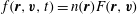 $f(\boldsymbol{r},\boldsymbol{v},t)=n(\boldsymbol{r})F(\boldsymbol{r},\boldsymbol{v})$
, which is reconstructed using the dust number density,
$f(\boldsymbol{r},\boldsymbol{v},t)=n(\boldsymbol{r})F(\boldsymbol{r},\boldsymbol{v})$
, which is reconstructed using the dust number density,
 $n(\boldsymbol{r})$
, measured using the image data, and the velocity distribution function,
$n(\boldsymbol{r})$
, measured using the image data, and the velocity distribution function,
 $F(\boldsymbol{r},\boldsymbol{v})$
, measured using PIV techniques. While it is the case that a key feature of the PIV technique is that it reports the velocity of a cluster of particles, not the velocity of individual particles, a mapping function that accounts for the intrinsic averaging that takes place when performing the PIV analysis has been developed through extensive simulations of the PIV measurement technique (Williams Reference Williams2006). In particular, this mapping function provides a numerical factor that depends on the local number density that can be applied to the measured velocity distribution to account for the averaging that takes place when performing the PIV analysis and returns the underlying velocity distribution function of the dust particles. This mapping function has been benchmarked using both simulated (Thomas Jr, Williams & Räth Reference Thomas, Williams and Räth2010) and experimental data (see supplementary material available at http://dx.doi.org/10.1017/S0022377816000507), allowing one to recover the underlying velocity distribution function from what is measured using PIV techniques. Once the phase space distribution function has been reconstructed, it can then be modelled using an appropriate distribution function, such as the tri-normal distribution (Fisher & Thomas Jr Reference Fisher and Thomas2011, Reference Fisher and Thomas2012), and moments can be taken to find the thermal properties of the dust cloud. Results from this analysis approach applied to tomographic PIV measurements of a dust cloud composed of
$F(\boldsymbol{r},\boldsymbol{v})$
, measured using PIV techniques. While it is the case that a key feature of the PIV technique is that it reports the velocity of a cluster of particles, not the velocity of individual particles, a mapping function that accounts for the intrinsic averaging that takes place when performing the PIV analysis has been developed through extensive simulations of the PIV measurement technique (Williams Reference Williams2006). In particular, this mapping function provides a numerical factor that depends on the local number density that can be applied to the measured velocity distribution to account for the averaging that takes place when performing the PIV analysis and returns the underlying velocity distribution function of the dust particles. This mapping function has been benchmarked using both simulated (Thomas Jr, Williams & Räth Reference Thomas, Williams and Räth2010) and experimental data (see supplementary material available at http://dx.doi.org/10.1017/S0022377816000507), allowing one to recover the underlying velocity distribution function from what is measured using PIV techniques. Once the phase space distribution function has been reconstructed, it can then be modelled using an appropriate distribution function, such as the tri-normal distribution (Fisher & Thomas Jr Reference Fisher and Thomas2011, Reference Fisher and Thomas2012), and moments can be taken to find the thermal properties of the dust cloud. Results from this analysis approach applied to tomographic PIV measurements of a dust cloud composed of
 $1.98~{\rm\mu}\text{m}$
diameter melamine microspheres suspended in an argon dc glow discharge plasma are seen in figure 8. Here, the recovered velocity distribution function,
$1.98~{\rm\mu}\text{m}$
diameter melamine microspheres suspended in an argon dc glow discharge plasma are seen in figure 8. Here, the recovered velocity distribution function,
 $F(\boldsymbol{r},\boldsymbol{v})$
, was modelled using a tri-normal distribution and it was observed that the kinetic temperature of the dust component was asymmetric and larger than the other plasma species. While these results are consistent with previous measurements, it is noted that the larger temperature of the dust component does not tell the full story. In particular, the number density of the dust component is significantly lower than the other plasma species which suggests that the contribution of the dust component to the (thermal) energy balance of the system is not as significant as is implied by the relatively large temperatures. If one considers instead the thermal energy density (Fisher et al.
Reference Fisher, Avinash, Thomas, Merlino and Gupta2013), a more complete metric of the energy density that includes a measure of the energy associated with the random motion and information about the number density, one can then compare the relative contribution of the different plasma species to the thermal state of the plasma system. Here, it was observed that the thermal energy density of the dust component is comparable to the other plasma species. However, it is also observed that the energy density (figure 8
b), is significantly larger in the presence of the dust acoustic wave, results that are consistent with previous measurements (Williams & Thomas Jr Reference Williams and Thomas2007; Fisher & Thomas Jr Reference Fisher and Thomas2011, Reference Fisher and Thomas2013; Fisher et al.
Reference Fisher, Avinash, Thomas, Merlino and Gupta2013). It is also possible to find the thermal energy flow rate from moments of the phase space distribution function (figure 8
c). It is observed that there is a significant amount of energy transport within the cloud and that this energy transport is correlated with the wave structure. These measurements provide insight into the volumetric nature of energy transport in weakly coupled dusty plasmas, highlighting a unique measurement capability of the tomographic PIV technique.
$F(\boldsymbol{r},\boldsymbol{v})$
, was modelled using a tri-normal distribution and it was observed that the kinetic temperature of the dust component was asymmetric and larger than the other plasma species. While these results are consistent with previous measurements, it is noted that the larger temperature of the dust component does not tell the full story. In particular, the number density of the dust component is significantly lower than the other plasma species which suggests that the contribution of the dust component to the (thermal) energy balance of the system is not as significant as is implied by the relatively large temperatures. If one considers instead the thermal energy density (Fisher et al.
Reference Fisher, Avinash, Thomas, Merlino and Gupta2013), a more complete metric of the energy density that includes a measure of the energy associated with the random motion and information about the number density, one can then compare the relative contribution of the different plasma species to the thermal state of the plasma system. Here, it was observed that the thermal energy density of the dust component is comparable to the other plasma species. However, it is also observed that the energy density (figure 8
b), is significantly larger in the presence of the dust acoustic wave, results that are consistent with previous measurements (Williams & Thomas Jr Reference Williams and Thomas2007; Fisher & Thomas Jr Reference Fisher and Thomas2011, Reference Fisher and Thomas2013; Fisher et al.
Reference Fisher, Avinash, Thomas, Merlino and Gupta2013). It is also possible to find the thermal energy flow rate from moments of the phase space distribution function (figure 8
c). It is observed that there is a significant amount of energy transport within the cloud and that this energy transport is correlated with the wave structure. These measurements provide insight into the volumetric nature of energy transport in weakly coupled dusty plasmas, highlighting a unique measurement capability of the tomographic PIV technique.
4 Future directions
Since the initial introduction of the PIV technique in the study of dusty plasmas, there have been significant advances in imaging and computational technology. These advances have been critical to the development of increasingly sophisticated PIV analysis techniques, resulting in the ability to (1) make measurements with greater temporal resolution, (2) take more complete measurements of the volumetric nature of the particle transport and (3) make this technique accessible without the need for a dedicated PIV system. While there has been great progress, there remain many potential future directions for the application of this technique. In this section, we highlight a few of these potential future directions for the development of this diagnostic technique in the study of dusty plasmas.
4.1 Uncertainty quantification
In the application of the PIV technique, there are a number of potential sources of uncertainty, including noise in the acquired images (Huang, Dabiri & Gharib Reference Huang, Dabiri and Gharib1997), the number density of the particles in the acquired images, peak locking that occurs due to the use of small particles (Westerweel Reference Westerweel1997; Christensen Reference Christensen2004), particle motion that is perpendicular to the illumination plane (Nobach & Bodenschatz Reference Nobach and Bodenschatz2009) and the existence of velocity gradients (Meunier & Leweke Reference Meunier and Leweke2003; Westerweel Reference Westerweel2007). Many of these issues have been extensively examined by the fluid mechanics community through modelling the measurement process (Westerweel Reference Westerweel1997) or through the use of Monte Carlo simulations (Keane & Adrian Reference Keane and Adrian1992; Fincham & Delerce Reference Fincham and Delerce2000; Scarano & Riethmuller Reference Scarano and Riethmuller2000; Lecordier et al. Reference Lecordier, Demare, Vervisch, Réveillon and Trinité2001). The results of these efforts have shown that the error associated with the PIV technique is typically between 0.03 and 0.1 pixel (Raffel et al. Reference Raffel, Willert, Wereley and Kompenhans2007). However, it is also known that the Monte Carlo simulations can underestimate the errors that are observed in experiments (Stanislas et al. Reference Stanislas, Okamoto, Kähler and Westerweel2005). As a result, the fluid mechanics community has recently developed a number of techniques to assess the uncertainty in the measured velocity field using information that is available in the experimental data (i.e. the images used in the PIV analysis, the cross-correlation function and the velocity vectors). These methods include the uncertainty surface method (Timmins et al. Reference Timmins, Wilson, Smith and Vlachos2012), the particle disparity method (Sciacchitano, Wieneke & Scarano Reference Sciacchitano, Wieneke and Scarano2013), the peak ratio method (Charonko & Vlachos Reference Charonko and Vlachos2013) and the correlation statistics method (Wieneke Reference Wieneke2015). While each of these methods has strengths and limitations (Sciacchitano et al. Reference Sciacchitano, Wieneke and Scarano2013), it has also been shown that the uncertainty in the measured velocity field tends to vary across the measurement region and that the significance of each of the previously noted sources of uncertainty contributes different amounts to the total measurement uncertainty depending on the experimental conditions (Neal et al. Reference Neal, Sciacchitano, Smith and Scarano2015; Sciacchitano et al. Reference Sciacchitano, Neal, Smith, Warner, Vlachos, Wieneke and Scarano2015). Given that the application of PIV techniques to a dusty plasma does not meet the same conditions/criteria that are typically seen in a fluid experiment, it is necessary to perform a similar comparison on data from the dusty plasma community to provide a more accurate measure of the uncertainty that is present is the resulting velocity fields.
4.2 Time-resolved stereoscopic PIV
Advances in imaging technology, particularly the availability of higher frame-rate cameras, have made it possible to analyse data from a wide range of laboratory and microgravity experiments using the PIV technique. As a result, the planar PIV technique has been adapted and applied to a wide range of experimental data acquired using the conventional diagnostic system within the dusty plasma community. However, as previously noted, there are limitations to the planar PIV approach. Additionally, the dedicated systems that employ the more sophisticated PIV approaches (i.e. stereoscopic and tomographic PIV) that have been used in the study of dusty plasmas have limited temporal resolution (
 ${\leqslant}15~\text{Hz}$
). Given the three-dimensional nature of many dusty plasma systems and the need for better temporal resolution to better understand the transport and thermal properties of dusty plasmas, particularly those in a weakly coupled state, there is a need for a diagnostic system that can recover the three-dimensional motion with greater temporal resolution than currently exists. One way to address this need in the immediate term would be to leverage advances in high-speed imaging to develop a time-resolved stereoscopic PIV system using the work that has been done in adapting the planar PIV technique for use on data from the conventional diagnostic system within the dusty plasma community as a roadmap for the development of this new diagnostic approach.
${\leqslant}15~\text{Hz}$
). Given the three-dimensional nature of many dusty plasma systems and the need for better temporal resolution to better understand the transport and thermal properties of dusty plasmas, particularly those in a weakly coupled state, there is a need for a diagnostic system that can recover the three-dimensional motion with greater temporal resolution than currently exists. One way to address this need in the immediate term would be to leverage advances in high-speed imaging to develop a time-resolved stereoscopic PIV system using the work that has been done in adapting the planar PIV technique for use on data from the conventional diagnostic system within the dusty plasma community as a roadmap for the development of this new diagnostic approach.
4.3 Combining PIV and PTV analysis techniques
The PIV and PTV techniques have been the primary diagnostic techniques used in the study of dusty plasmas. While the most appropriate analysis technique is determined based on the number density and observed particle motion in the acquired images, there are cases where these techniques can be used simultaneously to gain greater insight (Williams et al. Reference Williams, Thomas, Couëdel, Ivlev, Zhdanov, Nosenko, Thomas and Morfill2012). This presents a new direction for the analysis of data from dusty plasma experiments, one where the PTV and PIV techniques are used in tandem to gain greater insight into the underlying physics. Additionally, it is possible that these diagnostic approaches could be merged to provide a single diagnostic tool for the study of dusty plasmas. One approach would be to perform an initial analysis using the PIV technique to find a robust estimate of the local velocity field. This local velocity field would be used in the PTV analysis to predict particle positions, reducing the number of possible particle pairs and the number of false measurements. A second approach would be to develop a single code that would determine which technique would be most appropriate based on the number density and particle motion in the acquired images before performing the analysis. Both of these approaches would require the development and benchmarking of new analysis codes but could provide a valuable diagnostic tool to the dusty plasma community.
4.4 Plenoptic PIV
Plenoptic PIV (Fahringer, Lynch & Thurow Reference Fahringer, Lynch and Thurow2015) is a developing technology that is based on light-field imaging. This imaging approach was first proposed in 1908 (Lippmann Reference Lippmann1908) and is based on the idea that the propagation of a light-ray is represented by a five-dimensional function, known as the light field, that describes the location of the light-ray in space,
 $(x,y,z)$
, the direction of the light-ray’s propagation,
$(x,y,z)$
, the direction of the light-ray’s propagation,
 $({\it\theta},{\it\phi})$
and the wavelength of the light-ray,
$({\it\theta},{\it\phi})$
and the wavelength of the light-ray,
 ${\it\lambda}$
. When applying this principle to PIV, it is often the case that a single wavelength is used when acquiring the image data and that the intensity of the light is constant. As a result, the light field reduces to a four variable function,
${\it\lambda}$
. When applying this principle to PIV, it is often the case that a single wavelength is used when acquiring the image data and that the intensity of the light is constant. As a result, the light field reduces to a four variable function,
 $L(x,y,{\it\theta},{\it\phi})$
. In conventional imaging, a camera lens collects light over a range of angles, focusing the light onto the imaging sensor, effectively integrating the signal and resulting in only two of the relevant dimensions of the light field,
$L(x,y,{\it\theta},{\it\phi})$
. In conventional imaging, a camera lens collects light over a range of angles, focusing the light onto the imaging sensor, effectively integrating the signal and resulting in only two of the relevant dimensions of the light field,
 $(x,y)$
, being measured. In the stereoscopic and tomographic PIV approaches previously described, the information that is gained by the use of additional cameras and the empirical calibration function relating the orientation of the cameras and illumination region are used to reconstruct the four-dimensional light field to recover the full three-dimensional motion.
$(x,y)$
, being measured. In the stereoscopic and tomographic PIV approaches previously described, the information that is gained by the use of additional cameras and the empirical calibration function relating the orientation of the cameras and illumination region are used to reconstruct the four-dimensional light field to recover the full three-dimensional motion.
A plenoptic, or light-field, camera measures the full light-field function by placing an array of short focal length micro lenses at the focal length of the camera lens in front of the imaging sensor. Each microlens determines the position
 $(x,y)$
of a light-ray collected by the main camera lens, and then projects the light-ray onto an array of pixels, allowing for the direction of the light-ray’s propagation,
$(x,y)$
of a light-ray collected by the main camera lens, and then projects the light-ray onto an array of pixels, allowing for the direction of the light-ray’s propagation,
 $({\it\theta},{\it\phi})$
, to be determined. The result is a complete measurement of the light field,
$({\it\theta},{\it\phi})$
, to be determined. The result is a complete measurement of the light field,
 $L(x,y,{\it\theta},{\it\phi})$
, and an image that can be refocused at any plane in the depth of field, allowing for a fully volumetric measurement with a single camera. When applied to dusty plasmas, it could be possible to fully reconstruct the three-dimensional intensity field that represents the illuminated volume and a volumetric cross-correlation can then be performed to find a complete three-dimensional transport of the dust component. A key advantage is that this would require only a single camera. While this technology is still being developed, promising results have been seen within the fluid mechanics community (Thurow et al.
Reference Thurow, Fahringer, Johnson and Hellman2014; Deem et al.
Reference Deem, Agentis, Nicolas, Cattafesta, Fahringer and Thurow2015). This approach represents a promising diagnostic technique that has the potential to provide a complete measurement of the particle transport in a way that is notably more simple than the techniques currently employed.
$L(x,y,{\it\theta},{\it\phi})$
, and an image that can be refocused at any plane in the depth of field, allowing for a fully volumetric measurement with a single camera. When applied to dusty plasmas, it could be possible to fully reconstruct the three-dimensional intensity field that represents the illuminated volume and a volumetric cross-correlation can then be performed to find a complete three-dimensional transport of the dust component. A key advantage is that this would require only a single camera. While this technology is still being developed, promising results have been seen within the fluid mechanics community (Thurow et al.
Reference Thurow, Fahringer, Johnson and Hellman2014; Deem et al.
Reference Deem, Agentis, Nicolas, Cattafesta, Fahringer and Thurow2015). This approach represents a promising diagnostic technique that has the potential to provide a complete measurement of the particle transport in a way that is notably more simple than the techniques currently employed.
5 Summary
Over the past 20 years, the PIV technique has proven to be a useful diagnostic tool in the study of dusty plasmas, particularly when applied to dusty plasma systems with higher number densities or systems exhibiting fluid-like behaviour. This manuscript has presented the basic principles of this diagnostic technique, an overview of the PIV techniques that have been used in the study of dusty plasmas and a small sampling of measurements that are facilitated by this measurement technique. In doing so, we have highlighted a number of the strengths of this diagnostic technique. In particular, the PIV technique
-
(i) provides a computationally efficient means to rapidly reconstruct the two- and three-dimensional particle transport on a grid over the camera’s field of view with good spatial resolution and sub-pixel resolution of particle displacements (
 ${\sim}$
0.1 pixel);
${\sim}$
0.1 pixel); -
(ii) facilitates measurements of particle motion at higher number densities than is possible when using particle tracking techniques;
-
(iii) can provide detailed measurements of collective behaviour (i.e. waves, vortices, flows etc.) and thermal states of dusty plasmas;
-
(iv) can be applied to image data not acquired using dedicated systems provided that the image data is of sufficiently good quality and the timing used in image acquisition is well known; and
-
(v) can distinguish between particle-like and fluid-like behaviour depending on the time between the images analysed.

Additionally, the limitations of this technique have also been noted. In particular, the PIV technique
-
(1) does not provide the motion of individual particles. Instead, a reconstructed velocity vector represents the motion of a group of particles;
-
(2) can recover three-dimensional motion, but this requires the use of more sophisticated experimental set-ups. For systems employing only one camera, the motion in the plane perpendicular to the illuminated place is currently lost; and
-
(3) works best for systems with reasonable and directed particle displacement and higher number densities. As a result, it is most useful when applied to fluid-like systems and is not particularly well-suited for use on systems in the strongly coupled regime.
Further, it has been shown that over the 20 years during which this technique has been used, advances in imaging technology and the introduction of more sophisticated PIV techniques have resulted in a general movement toward more complete measurements of particle transport in both the temporal and spatial domains. Taken together, there are several opportunities for researchers to make use of this diagnostic technique and several areas for advancement in understanding the properties of this technique when applied to dusty plasma systems.
Acknowledgements
The author would like to thank Professor E. Thomas, Jr. of Auburn University, AL, for useful discussions during the preparation of this manuscript and is grateful for the support of the US National Science Foundation under grant PHY-0953595.
Supplementary material
Supplementary material is available at http://dx.doi.org/10.1017/S0022377816000507.


