


Introduction
Coffee is an important economic sector for Colombia in terms of exports, agricultural land use, and job creation. Annual shipments of coffee were 6.6Footnote 1 percent of the country's total exports in 2017, and coffee plants covered 13.81Footnote 2 percent of the arable area of Colombia, which is the highest percentage of any single crop. Within Colombia, coffee directly employs 26 percent of all agricultural workers and provides income to more than 550,000 families living in 595 municipalities (Muñoz Ortega Reference Muñoz Ortega2014). Moreover, coffee-growing regions enjoy a higher standard of livingFootnote 3 and relatively low levels of income inequality compared to noncoffee growing regions (Departamento Nacional de Planeación [DNP] 2013).
In the international coffee market, Colombia has been an important participant in terms of global production and exports. Between 2010 and 2017, Colombia produced an average of 7.6 percent of global physical coffee production and exported an average of 8.9 percent of world coffee exports by volume, surpassed only by Brazil and Vietnam (International Coffee Organization (ICO) 2020).Footnote 4 During the same period, Colombia exported, on average, 86.3 percent of its coffee production, with the United States and the European Union buying 72 percent of Colombian coffee exports (ICO 2020; Federación Nacional de Cafeteros de Colombia (FNC) 2020c).
Despite the coffee sector's current importance for the Colombian economy, its share in the GDP has declined over the last few decades. In the late 1970s, coffee production accounted for roughly 1.64Footnote 5 percent of Colombia's GDP, declining to 0.73 percent of the GDP in 2017 (Departamento Administrativo Nacional de Estadística (DANE) 2018). The decline in the coffee share of GDP mirrored a broader decline in Colombia's overall agriculture share of GDP. The agricultural share of GDP fell from 22 percent in the late 1970s to 7 percent in 2017 (DANE 2018), reflecting a classical development path of moving away from agriculture and rural lifestyle in general.
Specifically, for Colombia, the economy experienced structural changes that reflected variations in the importance of different sectors in the GDP. Between 1975 and 2017, the Colombian economy saw an allocation of resources away from the agricultural and manufacturing sector. These resources were principally moved toward the service sector (i.e., financial, insurance, real estate, and other services offered to businesses), followed by an increasing importance of the mining sector in the Colombian economy. Ocampo-Gaviria and Romero-Baquero (Reference Ocampo-Gaviria, Romero-Baquero and Ocampo-Gaviria2015) discuss the structural changes in the GDP composition being attributed to the economic liberalization that included structural changes in exports and restructuring of the financial sector. Exports became more diversified and less dependent on coffee. The increased export diversification included a greater participation of the mining sector, thanks to its growth and favorable international prices. The restructuring of the financial sector included elimination of restrictions on foreign capital, elimination of forced credit and investment policies for different economic sectors, and privatization of government-owned financial institutions. Ocampo-Gaviria and Romero-Baquero (Reference Ocampo-Gaviria, Romero-Baquero and Ocampo-Gaviria2015) indicate that in addition to economic liberalization, changes in the sectoral participation in the GDP were also attributed to the greater private participation in sectors traditionally reserved to the government, changes in the standard of living, and income distribution.Footnote 6
Several scholarly articles have focused on the decline of the agricultural share of GDP in the course of economic growth (Anderson Reference Anderson1987; Martin and Warr Reference Martin and Warr1993, Reference Martin and Warr1994; Sun, Fulginiti, and Peterson Reference Sun, Fulginiti and Peterson2007; Esposti Reference Esposti2012, Reference Esposti2014). Three major long-run driving forces have been identified as contributing to agriculture's decline compared with nonagricultural sectors, including (a) changes in relative prices of agricultural goods, (b) differences in the technical change rates between sectors, and (c) changes in factor endowments intensification across sectors.
There is no available literature addressing the reasons for the decline in the coffee sector in terms of the simultaneous effect of relative coffee prices, differential sectoral technical change, and changes in relative intensity in factor endowments of capital and labor. However, we can infer that the decline in the coffee share of GDP is associated with changes in coffee prices and the labor endowment. It has been well documented that coffee profits are sensitive to international coffee prices (Giraud-Héraud, Le Mouel, and Réquillart Reference Giraud-Héraud, Le Mouel and Réquillart1995; World Bank 2003). Declining coffee prices relative to other traded goods reduce coffee's share in the GDP due to valuation effects and resources shifting away from coffee toward sectors with greater returns (Martin and Warr Reference Martin and Warr1994). Low income elasticities of demand for agricultural goods relative to other traded goods (Martin and Warr Reference Martin and Warr1994; Muhammad et al. Reference Muhammad, Seale, Meade and Regmi2011; Esposti Reference Esposti2012) can potentially be attributed to the decline in the relative coffee prices. Furthermore, high-income countries are the largest world coffee consumers (Grigg Reference Grigg2002)Footnote 7 and have income elasticities of demand for agricultural goods 31 percent lower than low- and middle-income countries (Muhammad et al. Reference Muhammad, Seale, Meade and Regmi2011).
Similarly, a reduction in factor endowments can potentially be attributed to the decline in coffee output. With labor fleeing rural conflict zones in Colombia, the wages of the remaining workers rise, leading to higher costs for coffee producers (World Bank 2003). Labor costs account for 70–80 percent of coffee production costs with no offsetting improvement in labor productivity (World Bank 2003). Further, the shortage of rural labor leaves the coffee crop overly exposed to pests and not being harvested at the right time (Ocampo-Lopez and Alvarez-Herrera Reference Ocampo-Lopez and Alvarez-Herrera2017). As many farms in Colombia are located on steep slopes in the Andes Mountains, substituting capital for labor is problematic (Forero-Álvarez and Furio Reference Forero-Álvarez and Furio2010), resulting in lower yields per hectare compared with Brazilian and Vietnamese coffee farms. For example, the average coffee yield in the 2010–2017 period was 0.85 tons per hectare in Colombia, compared with 1.4 tons per hectare in Brazil and 2.35 tons per hectare in Vietnam (Food and Agriculture Organization of the United Nations (FAO) 2020).
We examine the declining coffee's share of GDP in Colombia by assessing the changes in relative prices, factor endowments, technological change, and three policy shocks affecting Colombia's economy. Those policy shocks are the collapse of the International Coffee Agreement (ICA) quota system in July 1989, the constitutional and legal reforms undertaken within Colombia between 1990 and 1994, and the 2016 peace agreement between the Revolutionary Armed Forces of Colombia (FARC)Footnote 8 and the Colombian government.
The ICA was an international commodity agreement between coffee-producing countries and consuming countries. First signed in 1962, the ICA maintained exporting countries' quotas and kept coffee prices high and stable. Empirical studies by Akiyama and Varangis (Reference Akiyama and Varangis1990) and Herrmann (Reference Herrmann1986, Reference Herrmann1988) suggest that the ICA was successful at raising the prices of coffee traded within the ICA. When ICA export quotas were suspended, producing countries lost most of their influence in the international market to increase coffee prices. The end of the quotas caused a sharp decline in international coffee prices as major exporters started to sell coffee aggressively (Giraud-Héraud, Le Mouel, and Réquillart Reference Giraud-Héraud, Le Mouel and Réquillart1995). The five-year average ICO composite price indicator fell from $1.34 per pound in the quota years (1984–1988) to an average of $0.77 per pound in the nonquota period (1990–1994) (Daviron and Ponte Reference Daviron and Ponte2005). Comparing the coffee share of GDP before and after the ICA, our data indicate that during the ICA quota period for the sample years (1975–1989), coffee production accounted for roughly 1.45 percent of Colombia's GDP. After the collapse of the export quotas, the coffee's share fell to an average of 0.97 percent in the 1990–2017 period (DANE 2018).
The second policy shock was the constitutional and legal reforms undertaken from 1990 to 1994, which pursued a clear opening and internationalization of Colombia's economy. The reforms included a Constituent Assembly that created the 1991 National Constitution, and structural/institutional reforms in labor and foreign exchange markets that impacted the finance and commercial sectors. The reforms drastically altered the public/private sector mix in the Colombian economy (Montenegro Reference Montenegro1995). Jaramillo (Reference Jaramillo2001) compares the determinants of changes in farmers' returns for different tradable crops before and after the market liberalization in the early 1990s. For a tradable commodity, such as coffee, farmers' returns fell primarily due to the negative impact of international coffee prices and the real exchange appreciation of the Colombian peso (Jaramillo Reference Jaramillo2001). In contrast, farmers' returns on nontradable crops increased (Jaramillo Reference Jaramillo2001). While a more detailed review of the literature that analyzes the ICAFootnote 9 and the reforms in the early 1990s is beyond the scope of this article, we explore these policy shocks having distinctive influences on the behavior of coffee's share of GDP.
Additionally, we empirically assess the effect of the 2016 peace agreement between the FARC and the government on the coffee share of GDP. The presence of the FARC has affected the agricultural sector by diluting the rural labor supply through the forced displacement of rural workers, changing farmers' on-farm work decisions, and recruiting rural workers. Forced displacement of rural workers is the result of violent attacks on the population, forced recruitment of minors, and economic road blocks such as illegal seizure of livestock and crops, and expropriation of land (Defensoría del Pueblo 2001; Fernandez, Ibáñez, and Peña Reference Fernandez, Ibáñez and Peña2011; Sánchez-Cuervo and Aide Reference Sánchez-Cuervo and Aide2013). Research of rural labor markets in Colombia has also shown that changes in the rural labor supply have been used as means of coping with violent shocks (Fernandez, Ibáñez, and Peña Reference Fernandez, Ibáñez and Peña2011). Fernandez, Ibáñez, and Peña (Reference Fernandez, Ibáñez and Peña2011) found that households in the rural areas of Colombia reduce their time spent on on-farm work and increase their supply of labor on nonagricultural activities in response to violent shocks. Another factor affecting the rural labor supply is the FARC's recruitment of rural workers for their guerrillas as an alternative of employment during economic downturns (Dube and Vargas Reference Dube and Vargas2013) or through coercion and intimidation (Saab and Taylor Reference Saab and Taylor2009; Dube and Vargas Reference Dube and Vargas2013). In addition to diluting the rural labor supply, the FARC has also appropriated public funds (Richani Reference Richani1997), stripping the agricultural sector of potential funds for rural development.
In terms of the coffee sector, the coffee-producing regions are strategically important to the FARC. Coffee production is geographically located in a corridor that links the center of the country to the pacific coast and the northeast part of the country (Defensoría del Pueblo 2001). The presence of the FARC in the coffee production area has not only diluted the rural labor supply, but it has also contributed to crop substitution. The FARC has contributed to the dilution of the coffee labor supply, as the migrant workforce required by the cyclical coffee economy has provided a pool of potential workers for illegal crops (Rettberg Reference Rettberg2010; Dube and Vargas Reference Dube and Vargas2013). Additionally, illegal crop production related to drug trafficking by the FARC has penetrated the formal economy, leading to the substitution of legal crops. Coca crops supported by the FARC are a profitable alternative to economic uncertainty in coffee production (Defensoría del Pueblo 2001). Greater profitability in coca production has resulted in coffee farmers selling their lands. Other coffee farmers have converted their lands to the cultivation of coca leaves (Rettberg Reference Rettberg2010). Consequently, the rural areas that saw coca production rise have become more violent (Angrist and Kugler Reference Angrist and Kugler2008), changing coffee growers' productive decisions. The risk of violence has been found to negatively impact the Colombian coffee grower's decision to continue coffee production and on the percentage of the farm allocated to coffee (Ibañez-Londoño, Muñoz-Mora, and Verwimp Reference Ibañez-Londoño, Muñoz-Mora and Verwimp2013).
This article fills a gap in the literature by analyzing the dynamic coffee sector behavior in conjunction with other agricultural output, while accounting for the effects that the ICA collapse, market liberalization policies, and the peace agreement process had on the evolution of the coffee share of GDP. Specifically, we analyze the effects of relative prices, factor endowments, technological change, the collapse of the ICA quota system, the liberalization of markets, and the peace agreement process on the change in the coffee share of GDP in Colombia. We estimate those effects using a Vector Error Correction model (VECM) that looks at both the short- and long-run dynamics. The long-run equilibrium results are used to estimate price, output, and Stolper–Samuelson elasticities.
The article is organized as follows: The next section discusses the economic theory to analyze the coffee and other agricultural output shares of GDP. The section that follows outlines the econometric model. The last two sections present the results and conclude with policy implications.
Economic theory
We assume that the Colombian economy is a three-sector, three-fixed-factor, small open economy with competitive equilibria in all input and output markets making all prices exogenous and independent of domestic demand (Esposti Reference Esposti2014).Footnote 10 The assumption of a small open economy is appropriate, given the participation of Colombia in world coffee production. Colombia's share of world coffee production fell from 12 percent in 1970 to 6.25 percent in 2011 (Cano et al. Reference Cano, Vallejo, Caicedo, Amador and Tique2012).
Following Kohli (Reference Kohli1978, Reference Kohli1990), Fox and Kohli (Reference Fox and Kohli1998), and Sun, Fulginiti, and Peterson (Reference Sun, Fulginiti and Peterson2007), we assume that the economy's aggregate technology is convex, exhibits constant returns to scale, has free disposability, and has nonincreasing marginal rates of substitution and transformation. Under profit maximization, the competitive equilibrium can be characterized as the solution to the problem of maximizing revenues subject to technology, endowment of domestic resources, and a vector of positive output prices at each point in time. Thus, the aggregate technology at time t can be represented by a Gross Domestic Product (GDP)Footnote 11 function—or revenue function—defined as follows:

where yt is a vector of final outputs (i.e., coffee (C), other agricultural outputFootnote 12 (A), and nonagricultural output (E)), pt is a vector of final output prices (i.e., $P_{\rm C}{\rm , \;}P_{\rm A}{\rm , \;}\;{\rm and}{\kern 1pt} \;P_{\rm E}$ ), xt is a vector of factor endowments (i.e., capital (K), labor (L), and land (R)), t is a proxy for technical change, and T t is the production possibilities set.Footnote 13
The solution to the revenue maximization problem given in equation 1 is a function of the exogenous output prices and the revenue maximizing output that depends on the factor endowments and technology (Esposti Reference Esposti2014). For the empirical functional form of the revenue maximizing solution, π(pt, xt, t), the Translog functional form was chosen. The Translog revenue functional form yields simple estimating equations for the coffee share of GDP and the share of GDP devoted to factor endowments. Differentiating the Translog revenue function with respect to the log of the price of outputs and invoking Hotelling (Reference Hotelling1932)'s lemma yield to the output shares of GDP as dependent variables (Kohli Reference Kohli1978). Similarly, the factor endowment shares of GDP are found by differentiating the Translog revenue function with respect to the log of factor endowments (Feenstra Reference Feenstra2016). The Translog functional form is also less restrictive than other popular functional forms such as the Cobb Douglas and the CES (Villezca-Becerra and Shumway Reference Villezca-Becerra and Shumway1992; Sadoulet and De Janvry Reference Sadoulet and De Janvry1995).
The Translog functional form for the GDP function, after omitting the time subscript for simplicity, is defined as
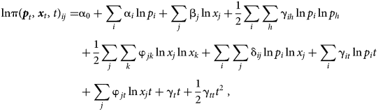
where $i{\rm , \;}h\in {\rm \{ }C{\rm , \;}A{\rm , \;}E{\rm \} and \;}\;j{\rm , \;}k\in {\rm \{ }L{\rm , \;}\;K{\rm , \;}\;R{\rm \} }$ . A system of output and input shares of GDP is derived from the Translog GDP function in equation 2 to analyze the effects of relative prices, factor endowments, and technological change on the coffee share of GDP. The output shares of GDP (Si) are derived by applying Hotelling (Reference Hotelling1932)'s lemma and imposing symmetry conditions to the Translog GDP function (Sun, Fulginiti, and Peterson Reference Sun, Fulginiti and Peterson2007; Esposti Reference Esposti2012). Thus, the ith output share of GDP is defined as follows:
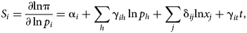
for i = C, A, E and where the symmetry conditions are γ ih = γ hi. Likewise, we can also find the inverse demand equations for the factor endowments in share form (V j) after imposing the symmetry conditions (Kohli Reference Kohli1978; Mckay, Lawrence, and Vlastuin Reference Mckay, Lawrence and Vlastuin1983; Feenstra Reference Feenstra2016). The share of GDP devoted to factor j is defined as follows:

For j = L, K, R and where the symmetry conditions are φjk = φkj. After imposing linear homogeneity in output prices and fixed inputs, the system of output and input shares of the GDP to estimateFootnote 14 is


where S E and V R can be estimated from equations 5 through 8 since output shares and input shares sum to one.
Econometric model
We estimate the system of equations 5–8 as a dynamic multiequational model where all variables are simultaneously determined and, therefore, endogenous. Vector autoregressive (VAR) models are used to study the dynamic interdependence between stationary time series. VAR models have been used to assess the impacts of agricultural prices, labor, land, and technological changes on the agricultural share of GDP (Esposti Reference Esposti2012, Reference Esposti2014) and the effect of agricultural production on economic growth (Tiffin and Irz Reference Tiffin and Irz2006). Other applications of VAR models in the agriculture sector include the assessment of energy price shocks (Wang and McPhail Reference Wang and McPhail2014), public research and development strategies (Esposti Reference Esposti2002), and the interdependence between agricultural commodity prices, land use, and food markets (Piroli, Ciaian, and Kancs Reference Piroli, Ciaian and Kancs2012; Pierre and Kaminski Reference Pierre and Kaminski2019).
However, spurious regression results can be obtained when regressing a nonstationary time series on one or more nonstationary series in the VAR model (Gujarati Reference Gujarati2015). A viable solution to deal with nonstationary time series is to estimate the VAR model in first differences if the time series are first-difference stationary. However, the VAR model in first differences is misspecified if the nonstationary time series obey a stationary equilibrium relationship (Statacorp LLC 2017), because the VAR model would only estimate short-run dynamics among the time series. Accordingly, the VAR model can be extended to a VECMFootnote 15 if the nonstationary time series follow a stationary equilibrium relationship or cointegration (Becketti Reference Becketti2013; Gujarati Reference Gujarati2015). In the VECM framework, the regression of a nonstationary series on another nonstationary series does not result in a spurious regression (Gujarati Reference Gujarati2015). Similar to the VAR model, the VECM fits the first differences of the nonstationary series, but a lagged vector of error-correction terms is added to represent the cointegration or long-term equilibrium relationships between the time series (Becketti Reference Becketti2013). The vector of error-correction terms represents short-term deviations from the long-term equilibrium relationships (Becketti Reference Becketti2013).Footnote 16
Assuming that long-term relationships (i.e., cointegration) between the variables exist, the dynamic simultaneous equation model can be specified as a VECM. Specifically, the VECM with lag order k is defined as follows:

where y is the p × 1 vector of variables, ɛ is a p × 1 vector of independent and identically normally distributed disturbances, and Δ denotes first differences. The vector y corresponds to the variables in the system of equations 5–8 which include S C, S A, V K, V L, log(P c/P E), log(P A/P E), log(L/R), and log(K/R). The long-term equilibria is defined by ${ \boldsymbol \beta }^{ {\prime}}{ \boldsymbol y}_{t\hbox{-} 1} + { \boldsymbol \mu} + { \boldsymbol \rho}\, t}$ , where β is a p × r matrix of cointegrating relationships, μ and ρ are r × 1 vectors of parameters, t is a time trend, and r is the number of cointegrating vectors. The short-run dynamics are defined by the p × r error correction matrix (i.e., α), the p × p coefficient matrix of short-run dynamic relationships between the elements of y (i.e., Γi), and a p × 1 vector of parameters γ. The error correction parameters, α, are interpreted as the adjustment speed in y to deviations from the long-run equilibria. The VECM, as defined in equation 9, restricts the cointegrating equations to be trend stationary (Statacorp LLC 2017).
In order to account for the structural break in equation 9, we introduce an intervention dummy following the discussion in Joyeux (Reference Joyeux and B. Bhaskara2007)Footnote 17. The VECM in equation 9 with a structural break is redefined as

where D t−k is the structural change or collapse of the quota system in 1989 and I t in the VECM framework accounts for the first difference in the structural change variable (Joyeux Reference Joyeux and B. Bhaskara2007). The structural change or intervention dummy, D t−k, takes the value of one for 1990 ≤ t ≤ 2017 and zero otherwise, and I t is a dummy variable taking the value of one for t = 1990 and zero otherwise. We also include three additional variables to account for major events: (1) a Policy90 variable accounting for the market liberalization changes in the early 1990s (equals one for the years 1990–1994 and zero otherwise),Footnote 18 (2) a ${\rm Peace}{\kern 1pt} \,{\rm Treaty}$ variable controlling for the effects of peace negotiations between the government and the FARC (equals one for the years 2012–2016 and zero otherwise), and (3) a Recession variable controlling for the Great Recession (equals one for the years 2008–2009 and zero otherwise).
Results
This study uses annual time-series data from 1975 to 2017 for the Colombian economy. Variable definitions, units of measurement, sources, and descriptive statistics are presented in Table 1. The annual average share of coffee and other agricultural output in the GDP is 1.1 percent and 11.4 percent, respectively. Descriptive data indicate a declining trend in the coffee share, other agricultural output share, and relative coffee and other agricultural output prices.
Table 1. Definition, descriptive statistics, and data sourcea
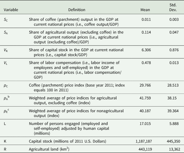
Data source: authors' calculation for S C, S A, p C, p A, and p E using data from the National Administrative Department of Statistics (DANE) and the National Planning Department (DNP) (DNP 2014; DANE 2018). V K was estimated using the value for capital stock, K, obtained from the Penn World Table 9.0 (Feenstra, Inklaar, and Timmer Reference Feenstra, Inklaar and Timmer2015) and the GDP data obtained from the DANE (DANE 2018). V L and L were obtained from the Penn World Table 9.0 (Feenstra, Inklaar, and Timmer Reference Feenstra, Inklaar and Timmer2015). R was obtained from the World Development Indicators (World Bank 2019).
a S C and S A were estimated by dividing the value of coffee output and agricultural output (excluding coffee) by the GDP, respectively. For example, for the period of analysis, on average, the coffee output value represented 1.14 percent of the GDP. Coffee production between 1975 and 1990 represented, on average, 1.45 percent of the GDP, while between 2000 and 2017 it represented, on average, 0.83 percent of the GDP.
b The price index for agricultural output (excluding coffee) was estimated as the weighted average of price indices with base year 2011 for: (1) other crop production, (2) animal production, and (3) forestry, fishing, and hunting. The weights were estimated by dividing each activity's output value (i.e., other crop production, animal production, and forestry/fishing/hunting) by the agricultural output.
c The price index for nonagricultural output was estimated as the weighted average of price indices with base year 2011, for the main classifications of nonagricultural economic activity. The weights were estimated by dividing each activity's output value by the GDP.
The empirical estimation of equation 10 consists of investigating the nonstationary nature of the variables and their first differences, testing for the number of cointegrating relationships, and identifying the lag order of the VECM. In this article, we examine the nonstationary relationship of the variables by investigating the existence of unit roots in the level of the variables as well as in their first differences using the modified Augmented Dickey–Fuller Test proposed by Elliott et al. (Reference Elliott, Rothenberg and Stock1996) (DF-GLS)Footnote 19 and the Innovational Outlier model unit root test proposed by Clemente et al. (Reference Clemente, Montañés and Reyes1998) (CMR-IO) tests. Both the DF-GLS and CMR-IO tests complement each other when investigating the nonstationarity of the variables. While both test for the unit root in the series, the CMR-IO test takes into account the presence of a structural break in the time series (Perron and Vogelsang Reference Perron and Vogelsang1992; Clemente, Montañés, and Reyes Reference Clemente, Montañés and Reyes1998). If the structural break is ignored, the unit root test can lose power (Perron Reference Perron1989). As noted by Zivot and Andrews (Reference Zivot and Andrews1992), the CMR-IO test helps identify a potential structural breakpoint time period as the test chooses the structural breakpoint that gives the least favorable result for the unit root null hypothesis.
Table 2 reports the unit root results for the levels and first differences in the data. The DF-GLS test indicates that the levels of all variables, except the relative price of coffee, are nonstationary. However, when allowing for a structural break, the CMR-IO test indicates that the levels of all variables, except the coffee share, other agricultural output share, and their relative prices are nonstationary. The CMR-IO test indicates that the coffee share, other agricultural output share, and their relative prices are stationary with a mean break in the early 1990s and in 2006. We conclude from the unit root tests on the level of the data that the time series for coffee share, other agricultural output share, and their relative prices are stationary with a structural break, while all other variables are nonstationary. The CMR-IO test suggests a break in the data in the early 1990s, which matches our expectation of a structural break due to the collapse of the ICA quota system and the market liberalization reforms. Furthermore, the CMR-IO test indicates a break in the data later in the 2000s, which we partly capture with a Great Recession dummy variable. Table 2 also indicates that the first differences of all variables are stationary, permitting us to use the first differences of the variables as the dependent variables in the VECM.
Table 2. Unit root tests
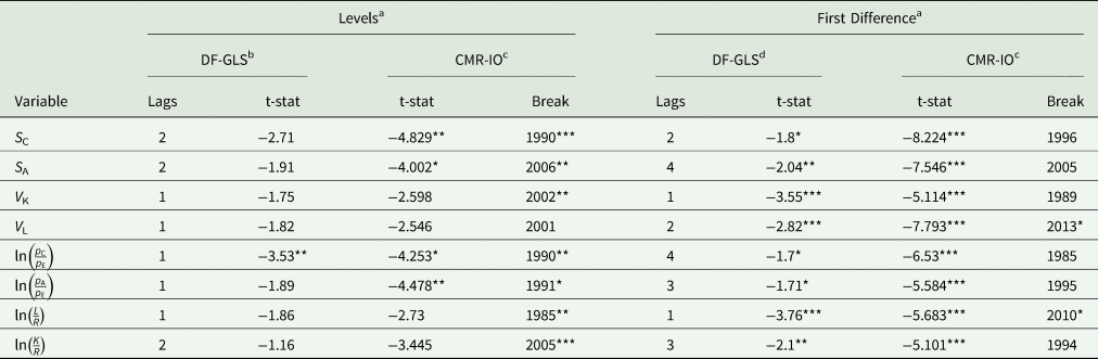
***, **, * indicate significant effects at the 1 percent, 5 percent, and 10 percent levels, respectively.
a Ng and Perron (Reference Ng and Perron1995) proposed a backward lag selection to minimize bias on the test. They proposed to select the lag such that the last lagged difference is significant (i.e., absolute value of the t-statistic for the last lag is greater than 1.6). Once the last lagged difference was found significant, the Modified Akaike Information Criterion (MAIC) was considered to select the number of lags to conduct the unit root test as proposed by Ng and Perron (Reference Ng and Perron2001). Ng and Perron (Reference Ng and Perron2001) show that the MAIC criterion is useful when using the DF-GLS test because of good power. The lag chosen for the CMR-IO test was the same lag reported by the MAIC criterion in the DF-GLS test.
b DF-GLS unit root test for the data in levels: Ho: unit root vs. Ha: trend stationary. DF-GLS test critical values (Elliott, Rothenberg, and Stock Reference Elliott, Rothenberg and Stock1996): −3.77 (1 percent level), −3.19 (5 percent level), and −2.89 (10 percent level).
c The CMR-IO model with one structural break was used to test for the unit root (Perron and Vogelsang Reference Perron and Vogelsang1992) where Ho: unit root with single structural break vs. Ha: stationary series with a single structural break. The CMR- IO model critical values are: −4.97 (1 percent level), −4.27 (5 percent level), and −3.86 (10 percent level).
d DF-GLS unit root test for the differenced data: Ho: unit root vs. Ha: level stationary. DF-GLS test critical values (Elliott, Rothenberg, and Stock Reference Elliott, Rothenberg and Stock1996): −2.633 (1 percent level), −1.95 (5 percent level), and −1.607 (10 percent level).
After investigating the nonstationary nature of the data, we test for the number of cointegrating equations which, in the VECM, determines the number of long-term relationships among the variables. Table 3 presents the results from Johansen's maximum likelihood cointegration test on equation 10 using the maximum eigenvalue statistic.Footnote 20 The null hypothesis of no cointegration is found to be rejected at the 5 percent significance level, indicating the existence of long-run or equilibrium relationships among the variables. The maximum eigenvalue statistic identifies two distinct cointegrating vectors.
Table 3. Johansen's maximum likelihood cointegration rank test in the presence of structural breaksa

** indicates significance at the 5 percent level. The number of cointegrating vectors is r.
a An intercept in the VAR model and a trend in the cointegrating equation were assumed. The Johansen's maximum likelihood cointegration rank test was conducted, assuming that the structural break was on 1989 and before the additional major events were included (i.e.,Policy90, ${\rm Peace}{\kern 1pt} \,{\rm Treaty}$ , and Recession variables). Excluding the additional mayor event variables allows us to follow the discussion on Joyeux (Reference Joyeux and B. Bhaskara2007) on testing for the number of cointegrating vectors in the presence of one structural break.
Lastly, we proceed to identify the lag order for the estimation of the VECM. Four different information criteria were used to investigate the lag order for the VECM (i.e., Likelihood Ratio (LR) test, Akaike (AIC), Schwarz's Bayesian (SBIC), and Hannan and Quin (HQIC)). The HQIC and the SBIC suggest a lag order of one, while the LR and the AIC suggest a lag order of two. Since the VECM estimates the first difference of the data, we use a lag order of two to estimate the VECM.
Long-run dynamics
Normalization restrictions are imposed to identify the two long-run cointegrating relationships suggested by Johansen's cointegration test. Given our interest in the output share equations to evaluate structural changes and elasticities, we impose the normalization restrictions to identify the share of coffee and other agricultural output. Furthermore, we assume that the discrepancy from the long-run equilibrium relationship in coffee and other agricultural output shares is corrected by the adjustment in those output shares. That is, within the cointegrating system, all variables, except S C and S A, are weakly exogenous.Footnote 21 After imposing the normalization and weakly exogenous conditions, the VECM of lag order two with two cointegrating relationships has stationary cointegrating relationships and the errors are normally distributed.Footnote 22
Tables 4 and 5 present the maximum likelihood estimates of the restricted long-run relationships and elasticity values obtained from the long-run estimates. The results in Table 4 indicate that own-relative prices and technological change are expected to significantly increase coffee and other agricultural output shares in the long run. Other results in Table 4 indicate capital intensity per agricultural land to be negatively associated with the Sector A share (i.e., agricultural output excluding coffee) in the long run.
Table 4. Maximum likelihood estimates of the long-run coffee and noncoffee/agricultural share in the GDPa
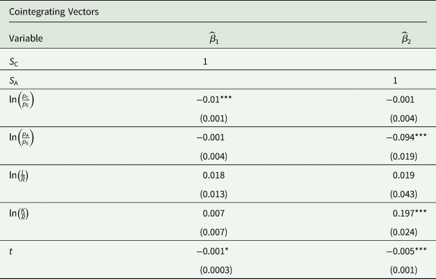
***, **, * indicates significant effects at the 1 percent, 5 percent, and 10 percent levels, respectively. Standard errors in parentheses.
a Normalization restrictions for the identification of the two cointegrating equations are: (1) cointegrating vector 1 normalizes S C (i.e., β11 = 1) and excludes S A, V K, and V L; (2) cointegrating vector 2 normalizes S A (i.e., β21 = 1) and excludes S C, V K, and V L. The two cointegrating vectors match the model specification in equations 5 and 6.
Table 5. Translog GDP function elasticity estimates for selected yearsa
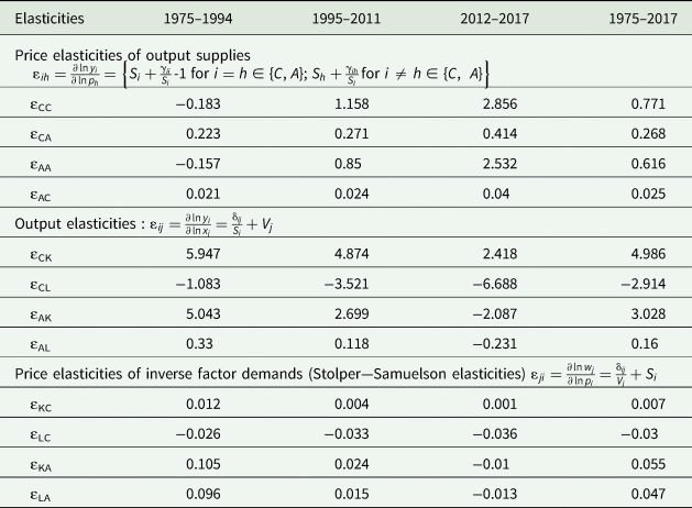
a The elasticity values were found at each time period and then averaged over the reference period. The estimation of elasticities follows the discussion on Feenstra (Reference Feenstra2016) and Mckay, Lawrence, and Vlastuin (Reference Mckay, Lawrence and Vlastuin1983).
Table 5 presents the estimation of different elasticities to assess the structural changes in the long run. Our result of the long-run elasticity of coffee supply is consistent with the long-run elasticity estimate of Akiyama and Varangis (Reference Akiyama and Varangis1990) for Colombia.Footnote 23 Before the major changes in the structure of the economy took place (i.e., 1975–1994), the results show negative, but small (in absolute value) own-price supply elasticities. The latter result seems counterintuitive, but should not be surprising, as during this period, the coffee market was highly regulated. Binswanger et al. (Reference Binswanger, Yang, Bowers and Mundlak1987) point out that negative supply elasticities could be the result of intertemporal optimization. That is, if there is an expectation of an increase in price to last into the future, producers find it desirable to build up inventory which reduces the present supply of coffee. For this reason, it is more informative to assess the own-price elasticities after the major structural changes happened in the Colombian economy.
After the major structural changes (i.e., after the 1989–1994 period) to the Colombian economy, agricultural output, including coffee, became more responsive to changes in their own prices. Specifically, our estimation suggests that coffee output became price-elastic after the market liberalization policies were introduced. Our results are consistent with the effect of the elimination of a quota system on the prices of agricultural commodities. For example, in a study on the effect of the end of coffee export quotas on price transmission in France, Germany, and the United States, Lee and Gómez (Reference Lee and Gómez2013) found that coffee retail prices became responsive to changes in international prices. In addition, our results indicate that the agricultural sector became even more responsive to its own prices during the period in which the peace negotiations between the government and the FARC took place.
The estimated cross-price elasticities of supply for coffee and Sector A (i.e., agricultural output excluding coffee) were all positive and inelastic, indicating that coffee and other agricultural output are complements in production. Coffee output supply increases when other agricultural output prices increase and vice versa. The latter result is consistent with the fact that coffee and other agricultural output international prices move together because of competition for land (de Gorter et al. Reference de Gorter, Drabik and Just2013). An exogenous increase in the relative price of coffee is usually accompanied by an increase in the price of other agricultural output.
However, for specific crops, cross-price elasticities of supply can be positive or negative depending on the degree of competition for inputs (e.g., labor and land) used on the production of such crops. For example, Ferreira Filho and Horridge (Reference Ferreira Filho and Horridge2014) found that policies increasing the demand for ethanol in Brazil stimulate the demand for sugarcane, resulting in higher prices for sugarcane. The greater price of sugarcane then influences the production of other crops depending on whether the competition for land with sugarcane is more or less intense (Ferreira Filho and Horridge Reference Ferreira Filho and Horridge2014). The results of Ferreira Filho and Horridge (Reference Ferreira Filho and Horridge2014) are consistent with negative and inelastic cross-price elasticities of output supply between sugarcane and coffee. Similarly, coffee is a close substitute for coca in terms of proper area conditions for growth (Muñoz-Mora, Tobón, and D'Anjou Reference Muñoz-Mora, Tobón and D'Anjou2018).Footnote 24
The long-run output elasticities presented in Table 5 give indirect evidence of the factor intensities used in production by defining the intensity of production in factor j as positive output elasticities (Feenstra, Hanson, and Swenson Reference Feenstra, Hanson and Swenson2000). Estimated output elasticities indicate that an increase in the endowment of capital favored all types of agricultural production before 1994. After the market liberalization reforms in the early 1990s, increases in the endowment of capital favored coffee production more than that of other agricultural output, as changes in capital had a larger impact on coffee output.
Long-run output elasticities also indicate that increases in labor (i.e., employment adjusted by human capital) did not favor coffee production. During the peace negotiations between the FARC and the government, coffee production was the most responsive to changes in labor. Additionally, the production of agricultural output (excluding coffee) (i.e., Sector A) went from positively responding to changes in labor in the period prior to the negotiations to negatively responding to changes in labor during the peace talks. The negative output elasticities for labor seem counterintuitive as agricultural goods are thought to be labor-intensive. However, since labor was measured by employment adjusted by human capital, our results show evidence of an educated labor force moving away from agricultural production (Huffman Reference Huffman1980).
The Stolper–Samuelson elasticities are the counterparts to the output elasticities (Kohli Reference Kohli1990) and allow us to assess the distributional effects of changes in the prices, all else equal. An increase in the price of coffee favors capital and hurts labor, with changes in the price of coffee having a less-than-proportional impact on the price of capital and labor. For all other agricultural output, increases in their price favored both capital and labor, except during the peace negotiations period.
Short-run dynamics
Tables 6 and 7 show how the share of coffee and other agricultural output is influenced in the short run by deviations from the long-run equilibrium and the short-term dynamics. Table 6 identifies the speed of adjustment parameters or the speed at which the share of coffee and other agricultural output responds to long-run deviations. The results indicate that about 50 percent of the long-run disequilibrium in the previous period's coffee share is corrected in one year by changes in its share contribution to the GDP. The agricultural sector (excluding coffee) significantly responds to long-run disequilibrium in its own share and the coffee share. That is, the agricultural sector's (excluding coffee) share completely adjusts in 6 months to correct for the long-run disequilibrium in the previous period's coffee share. Similarly, the agricultural sector's (excluding coffee) share completely adjusts in approximately 9 months to correct for the long-run disequilibrium in its previous period's share.
Table 6. The speed of adjustment coefficients
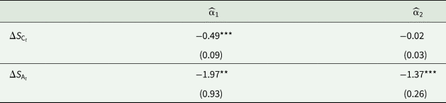
***, **, * indicates significant effects at the 1 percent, 5 percent, and 10 percent levels, respectively. Standard errors in parentheses. $\widehat{{\rm \alpha }}_i$ is the error correction parameter for the ith cointegration vector.
Table 7. Nonstructural maximum likelihood estimates of the dynamic short-run error correction model
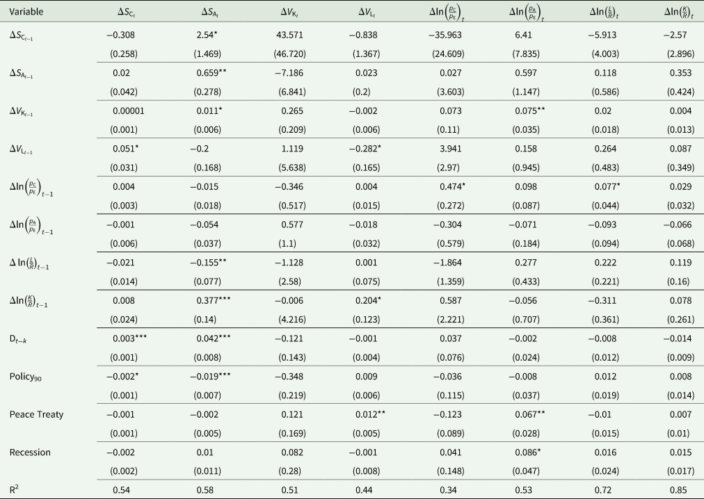
***, **, * indicates significant effects at the 1 percent, 5 percent, and 10 percent levels, respectively. Standard errors in parentheses.
Table 7 presents the results for the short-term estimated coefficients. For the coffee sector, coffee production responds positively to changes in the share of labor compensation in the GDP. All other agricultural output responds positively to changes in the economy's capital endowment. The impact of the collapse of the 1989 quota system and market reforms in the early 1990s had similar and stronger impacts in the agricultural sector (excluding coffee) relative to the coffee sector. The collapse of the quota system in 1989 had a small positive significant economic impact in both the coffee sector and the agricultural sector (excluding coffee). However, the market liberalization reforms in the early 1990s contributed to the overall decline in the agricultural sector. Our results indicate that it was the market liberalization reforms in the early 1990s and not the collapse of the quota system that acted as the policy shock contributing to the decline in the coffee share of GDP. Interestingly, other results indicate that the peace negotiations between the government and the FARC resulted in significant increases in the labor compensation share of GDP and the relative prices for the agricultural sector (excluding coffee). The 2008–2009 Great Recession significantly increased the relative prices of other agricultural output at the same time as the output share in the GDP continued to decline.
The other results from the short-dynamics estimates in Table 7 show that increases in relative coffee prices significantly increase the following period's labor intensity per land area. Increases in capital endowments are expected to significantly increase the agricultural sector (excluding coffee) relative prices and their output share in the GDP on the following period, while greater capital intensity per agricultural land area increases the labor share compensation on the following period.
Last, coffee output contribution to the GDP significantly increases all other agricultural output share in the GDP, which can be explained by the similarities in the trends in commodity prices due to competition for land and global macroeconomic trends (de Gorter, Drabik, and Just Reference de Gorter, Drabik and Just2013; Barbaglia, Wilms, and Croux Reference Barbaglia, Wilms and Croux2016). Our results intuitively support that global macroeconomic factors transmit faster to coffee production.
Conclusions
The importance of coffee for Colombia's economy goes well beyond coffee sales and employment. We used a Translog functional form for aggregate technology, and the results indicate that relative coffee prices and technological change significantly impact the share of coffee in the GDP in the long run. The short-run estimation results indicate that the decline in the coffee share cannot be attributed to the collapse of the coffee quota regime in 1989. Instead, the market liberalization and other regulatory reforms that took place in the early 1990s significantly reduced the size of the coffee sector in Colombia. The market liberalization and other regulatory reforms made coffee production more responsive to changes in the economy's employment and coffee prices. As market liberalization policies appeared to have a negative impact on coffee production, farmers continue to require assistance to compete in international markets.
A comparison of the returns for different tradable commodities before and after market liberalization polices, Jaramillo (Reference Jaramillo2001) shows that the returns for coffee fell due to the appreciation of the exchange rate and the negative impact of international prices. Two different programs have been implemented to mitigate the negative impact of low international coffee prices on coffee farm income. The first program is called the “specialty coffee” extension program, which is currently offered through the National Federation of Coffee Growers of Colombia (FNC)Footnote 25 with resources from the national government to help farmers produce specialty coffees (Ministerio de Agricultura y Desarrollo Rural 2020). The specialty coffee support extension program provides technical support for coffees that have differentiated characteristics of origin, preparation, or sustainable production (FNC 2020b). This allows coffee producers to obtain a greater price for their crop. Technical support provides assistance to meet the requirements of different seals, codes of conduct, and certifications that accredit the coffee as a specialty coffee (FNC 2020b).
The second program—Governmental Incentive for Coffee Equity (IGEC)Footnote 26 2019—lasted until December 2019 and provided income support to coffee producers. The IGEC 2019 program helped mitigate the negative impact that international markets had on farm income by providing a subsidy if the coffee's domestic reference price fell below an established price floor at the time of the physical sale (FNC 2019). The IGEC 2019 program protected coffee farmers from drops in the domestic reference price that is dependent on the price in the New York Stock Exchange, the quality premium recognized for Colombian coffee, and the exchange rate of the Colombian peso against the US dollar (FNC 2020a). Our results favor the continuation of income support programs such as the IGEC 2019 to counteract the negative impact of market liberalization policies on the coffee production share in the national GDP. Further, our results indicate that coffee and agricultural output (excluding coffee) are complements in production, with agricultural output (excluding coffee) responding to the coffee output's share contribution in the GDP. Coffee and other agricultural output are dependent on each other due to similarities in the way commodity prices trend, competition for scarce land, and global macroeconomic trends.
Other estimations in the short run indicate that coffee production responds positively to increases in the share of labor compensation in the GDP. In the framework of the peace accords signed in 2016 between the Colombian government and the FARC, specific rural labor reforms were included in the agreement with potential to improve the production of coffee. The peace accords support the strengthening of the rural labor market by facilitating access to employment rights, strengthening the labor inspection system, and providing provisions for an occupational risk subsidy (Office of the High Peace Commissioner 2017).
The importance of the coffee sector in the Colombian economy in terms of employment, standard of living for rural households, and lower levels of income inequality also highlights the importance of assessing the sector as a foundation for rural economic development. For example, illegal coca crop substitution policies need to be assessed in conjunction with coffee sector policies. Illicit drug prohibition policies directed to restrict the illicit drug supply have been found to generate political instability (Saenz and Barilla Reference Saenz and Barilla2020). Alternatively, in Colombia, coffee and coca can be considered close substitutes in terms of conditions for growth (Muñoz-Mora, Tobón, and D'Anjou Reference Muñoz-Mora, Tobón and D'Anjou2018), suggesting that increasing farmers' net return from producing coffee could reduce coca production. Therefore, an assessment of the spillover effects of policies supporting the production of coffee, such as farmers’ support programs to improve their ability to compete in international markets, and a strengthening of rural labor markets are important to generate economic stability in rural communities affected by armed conflicts.
Funding statement
This research received no specific grant from any funding agency, commercial, or not-for-profit sectors.
Conflict of Interest
None declared.


 Open access