


Introduction
Reference VoellmyVoellmy’s (1955) methods for computing avalanche speed and run-out distance have been used by engineers for many years, although not without reservations, some of which are explored in other papers at this Symposium. We will focus on certain difficulties in the Voellmy approach, difficulties that we believe can be remedied without further complicating the theory of avalanche dynamics, but rather by reworking the theory into a more concise and systematic form. To see what these difficulties are, we first restate briefly some of Voellmy’s underlying assumptions and central results.
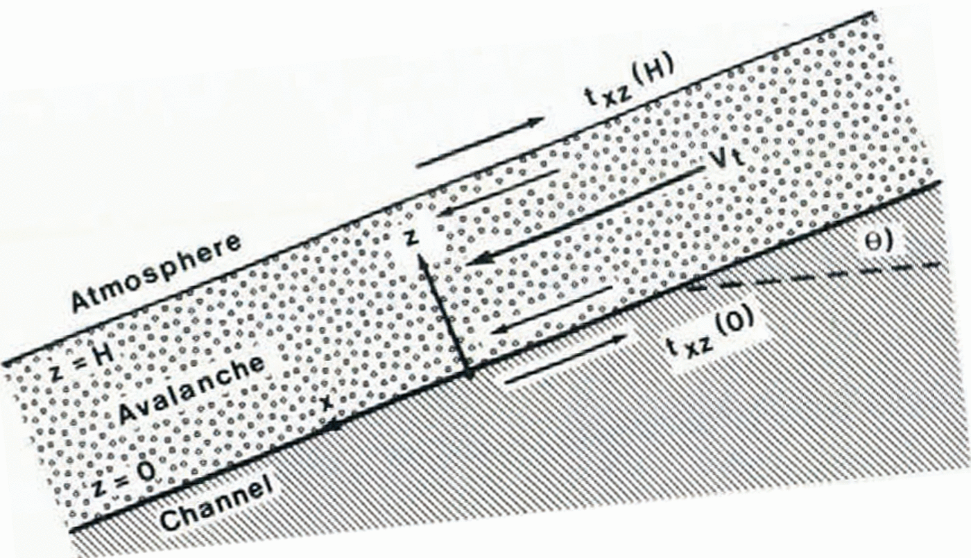
Fig. 1. Avalanche on long, inclined channel.
The foundation of Voellmy’s method is rooted in hydraulic theory, specifically, the theory of open–channel flow. The avalanche is modelled as a fluid which accelerates very quickly from rest to a steady, terminal velocity in a long, inclined channel. If the avalanche accelerates to a terminal velocity Vt through Eulerian coordinates fixed to the channel (Fig. 1), then along the centre of the channel, where ( ∂⁄∂x) = (∂⁄∂y) = 0, shear stress txz and gravitational stress are balanced according to the equilibrium equation

where p is the density of the avalanche “fluid” and θ is the inclination of the channel. Assuming an average p across a flow height H, integration of Equation (1) gives
where the shear stresses txz(H) and txz(o) at the respective boundaries z = H and z = 0 are determined from additional assumptions. Voellmy assumes the boundary shear stress at the avalanche—atmosphere interface (z = H) is due to dynamic drag, and is therefore proportional to Vt2. Thus,
where k 1 is a constant. Shear stress at the avalanche-channel interface (z = 0) is also assumed to consist of dynamic drag, but because the avalanche consists of lumps and blocks that slide and bounce, a “friction” term proportional to the normal stress tzz is included. Hence,
where k 2 is a constant and where μ is a “coefficient of friction”. The friction term, which does not play a role in the conventional theory of open channel flow, appears to be necessary in order to model the observation that avalanches accelerate on relatively steep slopes (tan θ > μ) and decelerate on less steep slopes (tan θ <μ). Substituting boundary conditions Equations (3) and (4) into Equation (2) gives Voellmy’s formula for avalanche terminal velocity
where density and drag coefficients are lumped together into a single constant ξ.
The preceding derivation can be generalized to account for avalanche channels of given cross–section by replacing H with the hydraulic radius, which is defined in the theory of open–channel flow as the flow cross–sectional area divided by the wetted perimeter. Further hydraulic analogies are discussed by Reference Leaf and MartinelliLeaf and Martinelli (1977).
Voellmy also proposed a formula for computing the run-out distance S required for an avalanche to decelerate from terminal speed Vt to rest. His equation, based on a balance of energy, is
where the run-out distance S is measured from a reference position on the slope and where the velocity Vt is computed according to Equation (5). The parameter H D is the mean deposition depth, and is introduced to account for the energy lost due to the pile–up of debris.
In practice, one of the difficulties with Voellmy’s method is the need to establish a reference position for the computation of S. There are many ways a reference can be chosen. For example, it may seem logical to select the slope position where tan θ ≈μ. The path geometry is thus approximated as two slopes of constant θ joined at this reference. The accelerating condition (tan θ> μ) applies to the upper slope, and the decelerating condition (tan θ < μ) applies to the lower slope. For this choice, the computed S–value could depend crucially on the μ–value, but as we will show later, μ–values cannot be determined to great precision due to certain theoretical difficulties. Looked at another way, Voellmy’s method is inconsistent in the sense that acceleration distance is not used to compute Vt, whereas deceleration distance S is one of the essential outputs.
In summary, we feel it is illogical to compute avalanche velocities and run-out distances on paths of complex geometry by selecting a priori the reference position that separates the acceleration and deceleration portion of the avalanche path. We are thus led in a natural way to conclude that the logical reference is the initial rest position of the system, the starting zone, and that the computation should proceed down–slope from this reference.
Centre–of–mass model
If the reference position is taken at the starting zone, then distance enters into the acceleration as well as the deceleration computations. That is, the avalanche accelerates from its initial rest position (υ = 0, s = 0, t = 0); reaches a maximum velocity υ = Vmax at some slope position s = S1, or alternatively at some time t =t1; and then decelerates to rest, Ʋ = O, at a second position s = S 2 or t = t 2.
To model this accelerating and decelerating behaviour, we will assume that the moving avalanche is enclosed by finite boundaries at any slope position (or any time). Equivalently, we assume the avalanche has a finite mass M(s) or M(t), where s or t characterizes the position in space or time of the centre of mass. Admittedly, in Nature, the boundaries and mass of an avalanche are usually poorly defined. Perhaps this is why Voellmy chose the opposite viewpoint and solved for the motion of a column in an “endless” fluid. On the other hand, the longer and hence more interesting avalanche paths are on the order of 103m long, yet we believe from our visual observations (no firm data presently available) that most of the avalanche mass at any time is confined to a length scale not greater than half the path length, and typically on the order of 102 m. Therefore, in our opinion, the centre–of–mass model is the more reasonable of the two diametrically opposed viewpoints. It does turn out, however, that this argument may be academic since we will show that the “ endless–fluid ” and “centre–of–mass” viewpoints lead to analogous results in many respects, at least as far as present data allow us to evaluate details of both models. The task of synthesizing these opposite viewpoints into a comprehensive avalanche model which predicts the position of the centre of mass as well as the diffusion of the fluid–like boundaries is a task left for future investigators equipped with better data.
The motion of the centre of mass is described by Newton’s law relating the momentum change to the sum of the applied forces, that is

where M, the mass of the avalanche, is continuously changing due to entrainment of new snow from the path, or due to deposition of snow onto the track. The tangential equation of motion on a curved path is
where s is the position of the centre of mass measured along the path from the reference position at the top of the path, υ is the tangential speed ds⁄dt, and the tangential resistive force R is the sum of drag, ploughing, and friction as illustrated in Figure 2.
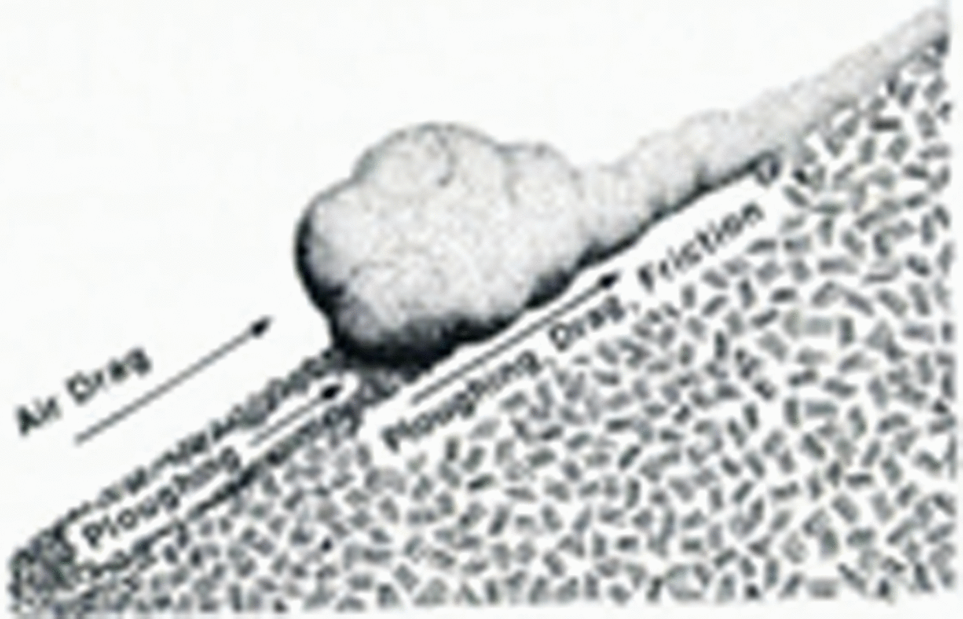
Fig. 2. Resistive forces opposing avalanche acceleration.
R has a complicated dependence on avalanche speed, shape, mass distribution, snow properties, path roughness, and related factors. As in Voellmy’s model, R is assumed to include a friction resistance proportional to the normal force against the path. If centripetal force is included, the friction component in R is
where μ is the coefficient of friction, and r is the local radius of curvature.
Also following Voellmy, the drag and ploughing terms in R are assumed to be dominated by an inertial term of the form kυ 2. This important assumption is examined later in our paper. Taking R as the sum of the friction term (9) and kυ 2, then substituting into Equation (8), and finally rearranging, gives

Note that entrainment is considered to have an inertial resistive effect, and is therefore lumped in with the other υ2 terms. After combining all υ2 terms into a single parameter

then Equation (10) can be expressed in the concise form

where solutions depend on two adjustable parameters μ and M⁄D. The latter parameter is given the physical interpretation of,a mass–to–drag ratio.
Equation (12) is a linear differential equation in υ2. Analytical solutions are cumbersome since the parametersθ, μ, and M⁄D are in general functions of position s. Instead, we use an iterative solution similar to the procedure proposed by Reference KörnerKörner (1976). First, we divide the slope into small enough segments that θ can be considered constant over the length of the segment. Each segment is assigned an angle θi, a length Li, a friction value μi and a mass/drag value (M⁄D)i. If the speed at the beginning of the ith segment is Vi A, and the avalanche does not stop somewhere in the middle of the segment, then the speed V i B at the end of the ith segment is the Equation (12) solution
where αi = g(sin θi—μi cos θi) and βi = —2Li⁄(M⁄D)i.
If the avalanche stops at a mid–segment position, the stopping distance S from the beginning of the ith segment is the Equation (12) solution

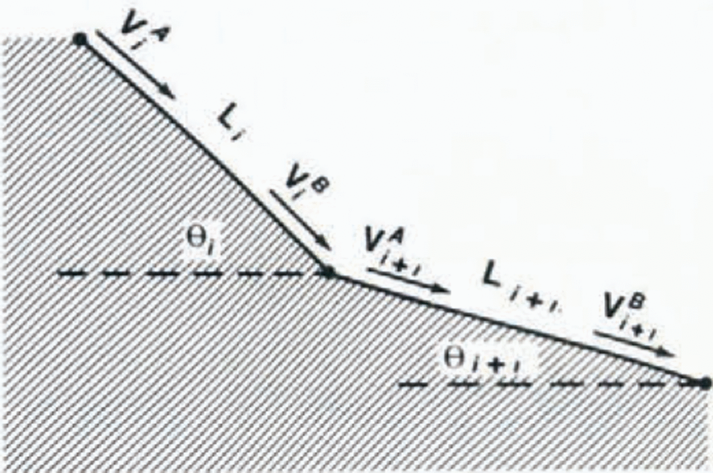
Fig. 3. Segmnt i and Segment i+1
As illustrated in Figure 3, the V i Bcomputed from Equation (13) is used to compute Vi+1A,and the computation repeated progressively down–slope until the stopping position, Vi B cannot always be substituted directly in place of Vi +1A, since it is sometimes necessary to include a correction for momentum change at the slope transition. For the case θi≥θi+1 we assume the following correction which is based on the conservation of linear momentum.
Equation (15) introduces a significant correction for an abrupt transition (e.g. an avalanche descending over a cliff onto benched terrain), but only a minute correction where a smooth curve is subdivided into many segments. For example, if a 450 are is divided into 100 segments the correction is cos100(45/100) ≈ 0.997. For the caseθi < θi+1,we envision that velocity decrease due to momentum change is compensated to a large extent by velocity increase due to the reduced friction as the avalanche tends to lift off the slope. Thus for the case θi < θi+1 we do not introduce a momentum correction, but simply set Vi+1A =Vi B.We recognize that our momentum corrections are only rough approximations that lose validity where the path of the centre-of-mass deviates significantly from the given slope profile.
The above computations were programmed for solution using a digital computer. Programming details are reported by Reference ChengCheng and Perla (1979). A sample computation for a simplified case where μ and M/Dare constant over the entire path length is shown in Table 1.
For the special case where μ and M⁄Dare constant on an infinitely long slope of constant inclination θ, and assuming the acceleration case tan θ > μ, then there is a maximum velocity solution to Equation (12) of the form

This result is analogous to Voellmy’s Equation (5), except that the factor Mg⁄Dreplaces the factor ξH.

The V 2 assumption
The square–root dependence common to both Voellmy’s Equation (5) and the centre–of–mass Equation (16) is a direct consequence of the assumption that R in both models has the special form a0+a2υ2. As Reference SalmSalm (1966) points out, the more general assumption is
where the coefficients a 0, a 1, and a 2 can be related to the respective effects of friction, viscous dissipation, and inertial resistance. The justification for selecting the term a 2υ2 rather than the term a 1υ is that at the speeds of interest, υ > 10 m⁄s, the Reynolds number should be sufficiently high that inertial effects involving stress terms proportional to ρυ2 should dominate the scale analysis of an equation of motion that includes both viscous and inertial stress terms. Air drag would involve a term proportional to ρυ2 where ρ is the density of air, while snow drag and ploughing would involve terms proportional to ![]() where ρ is now the density of undisturbed snow before drag and ploughing, and Δρ is the increase in snow density due to the comprcssional disturbance of drag and ploughing.
where ρ is now the density of undisturbed snow before drag and ploughing, and Δρ is the increase in snow density due to the comprcssional disturbance of drag and ploughing.
Setting aside the Reynolds number argument, there is some observational evidence to support the choice of an a 2υ2 term rather than an a 1υ term. If a 1υ dominated the equation of motion, then Vt would depend linearly on slope angle θ. However, Voellmy summarizes observations to the contrary: Vt varies weakly, if at all, with slope angle.
It is indeed fortunate that a 0┼a0υ2 appear to be the important terms, otherwise Equation (12) would be non–linear. Solutions for the three–parameter case a0┼a1υ┼a2υ2 given by Reference SalmSalm (1966) are still in advance of practical application. Even a two–parameter model is overly flexible and contains a mathematical redundancy, as we show later.
Range of μ and M⁄D
The values of μ and M⁄D (or Voellmy’s μ and ξH) can be estimated only roughly from existing data. Even the upper and lower bounds of μ and M⁄D (or ξH) are controversial. Voellmy claimed that μ could decrease to less than 0.1 if the avalanche fluidizes into a low density (c. 10 kg⁄m3) dust cloud. However, a value ofμ less than 0. 1 is difficult to reconcile with data collected by Reference Bovis and MearsBovis and Mears (1976), who found that the average slope angle in the deposition zone of large avalanches exceeds 10° (i.e.μ > 0.18). The only avalanches known to run steadily (without deceleration) on slopes where θ < 10° are slush avalanches, observed mostly in the Arctic.
The upper limit of μ is equally controversial, but it is known that avalanches have initiated from rest on 25° slopes (Perla, in press), and that after a, large avalanche begins accelerating it is unlikely to decelerate unless θ is less than 25°. These observations imply that μ is generally less than tan-1 25° or less than about 0.5. Thus, a reasonable range for μ appears to be 0.1 ≤ μ ≤ 0.5, depending on such factors as snow type, path roughness, and the presence of trees and obstacles.
The range of M⁄D (or Voellmy’s ξH) can be estimated from avalanche speeds using Equation (16) (or Voellmy’s Equation (5)). Speeds of large dry avalanches are reported by Voellmy and many others (Perla, in press) to sometimes reach 50 m⁄s, and possibly even reach 100 m⁄s. From Equation (16), it is seen that M⁄D must reach or exceed 103 m if avalanche speeds can truly exceed 50 m⁄s. Typically, wet avalanches move considerably slower (υ ≈ 10 m⁄s) and are thus characterized by lower M⁄D values (c. 102 m). The wide range of avalanche velocity indicates that the range of M⁄D (or ξH) spans several orders of magnitude, at least from 102 to 104 m, and possibly from 10 to 105 m.
Estimates of M and D
A more refined estimate of M⁄D could be based on separate estimates of M and D, in much the same way that Voellmy separates the factors ξ and H. Once again, we note that present data are so limited that we can only sketch order–of–magnitude estimates.
The avalanche mass M(s) is a function of position. The initial value M(0) is estimated as the mass of the snow in the starting zone, and the extreme values of M(0), for example the one-in-100-year estimate, determine the extreme values of velocity and run-out distance. Typically, M(o) is in the range 105 to 108 kg for the relatively larger avalanches that threaten facilities in North America. The values of M at successive segments down-slope from the starting zone depend on the rate of entrainment dM/ds. For convenience, Voellmy assumed dM/ds = o, but in Nature the deposited avalanche mass could be a multiple or a fraction of M (o). A relatively large avalanche, for example M(o) = 106 kg, could double its mass along a path length of 103 m, in which case (dM/ds) ≈ 103 kg/m. Entrainment rates could conceivably reach 104 kg/m, or perhaps higher for the world’s largest avalanches.
The parameter D also ranges widely depending on the terms in Equation (11), namely the drag and ploughing term k, the entrainment term dM/ds, and the curvature term μM/r. The curvature term (μM|r) presents an interesting problem because at cliff bands and terrain inflections, where r approaches zero, the curvature effect could easily dominate the M|D computation. For this reason, our computer solutions tacitly avoid the mathematical singularity of Equation (11). Instead, we approximate the avalanche path with straight-line segments and introduce a correction for momentum loss using Equation (15).
With curvature handled separately, the parameter D combines the remaining terms k and dM/s. Using conventional hydrodynamic theory, we estimate k as a sum of terms

where ρj is the density of the jth resistive medium the avalanche moves through (air, new snow, compressed snow), Aj is the portion of the avalanche surface area that interfaces with the jth medium, and Cj is a drag coefficient which is dependent on the shape of Aj and the Reynolds number. The density factor ρj ranges from 1 kg/m3 for air to over 1o2 kg/m3 for compressed snow. At the interface where the lead tip of the avalanche ploughs through snow, ρi is replaced by the term ![]() , discussed earlier.
, discussed earlier.
As example, consider a relatively large avalanche with M(o) ≈ 105 to 106kg. Typical values of Aj would range from 104 m2 at the avalanche—air interface, down to perhaps 102 m2 for the avalanche—snow interface at the lead or ploughing edge. From hydrodynamic tables, Cj will range from 0.1 to 1.0 for the Reynolds numbers, which are computed to exceed 105 using the traditional formula VL⁄v. On the basis of these estimates it is conceivable that k could range from 10 kg/m to 106 kg/m. However, in Equation (18), it is more likely that the air density 1 kg/m3 would pair with the large surface area 104 m2, and similarly the high density of the snow medium >102 kg/m3 would pair with the smaller surface area 102 m2. Hence, the range of k for this example of a relatively large avalanche is narrowed to perhaps 103 or 104kg/m, even allowing for variation in Cj and other uncertainties. Finally, recalling that our estimates of dM/ds overlap these estimates of k, we conclude that D (here, k+dM/ds) can also be estimated as c. 103 or 104 kg/m for the above example of a large avalanche,
Taking the example of the large avalanche one step further, we next combine our estimate 105 < M < 106 kg with the corresponding estimate 103 < D < 104kg/m, and obtain 102<M/D <103 m. This range is within the range derived independently in our previous section using velocity observations and Equation (16).
Suppose M(o) is significantly larger, for example c. 107 kg or c. 108kg. Does D also increase? In general, yes. A larger M implies a larger volume, which in turn implies larger surface area Aj along with higher dM/ds, and hence a higher D-value. However, M/D also increases in general since mass is proportional to L3, where L is some characteristic size, while surface area is proportional to L2, and thus M/D is proportional to L.
Voellmy introduced flow height H as a characteristic size in his Equation (5), but we feel that H is too restrictive to serve as the crucial parameter. Voellmy’s interpretation of the role of H breaks down if we no longer regard the avalanche as an “endless fluid” because at the front of the avalanche an increase in H due to fluidization implies an increase in frontal surface area. The increase in frontal resistive forces may have a decelerating effect, completely contrary to the prediction of Equation (5). It is for this reason we prefer the new parameter M/D which, compared to Voellmy’s ξH, allows a more flexible interpretation of the resistive forces
Numerical Computation of μ and M/d
It is possible to devise a criterion for calculating one pair {μ, M⁄D} or {μ, ξH} which matches the overall data measured on one or more paths. For example, Reference KörnerKörner (1976) has devised a graphical method for selecting the {μ, ξH} that best matches the known velocity and run-out distance for a single path. Since velocity data are rare, we pose another problem of practical importance: Find the pair {μ, M/D} which is the best predictor of known stopping positions for a group of N paths. Here it would seem that one could choose the {µ, M⁄D} which minimizes the difference between the computed and known stopping distance, summed for all N paths. However, this criterion will not work since a {μ, M/D} that yields a close fit for some of the paths may take the avalanche beyond the boundaries of the remaining paths in the group, and in some cases on towards “infinity” if tan θ >μ. To perform the calculations, we would therefore be forced to extend the paths in some arbitrary and artificial fashion. An alternative is to select {μ M/D} to minimize kinetic energy or impact pressure at the known stopping position. This is equivalent to selecting the {µ, M/D} that minimizes υ2 at the known stopping position. One way to proceed is as follows:
(a) If the avalanche is computed to overshoot the known stopping position, then compute υ 2 at the known stopping position.
(b) If the avalanche is computed to stop short of the known stopping position, then compute υ 2 necessary to force the avalanche from the “computed” to the known stop. This computation involves Equations (13), (14), and (15) applied in reverse.
(c) Assign positive values for the overshoot υ 2 (i.e. case (a)), negative values for the undershoot υ 2 (i.e. case (b)) and add algebraically for all N paths.
Table. II. CASCADE HIGHWAY AVALANCHES. From Reference LaChapelleLaChapelle and others (1971)
It is necessary to assign positive and negative values to the energy term (υ2), and to take an algebraic sum, because if instead the criterion is based on Σ |υ2|, then the optimum pair is perforce a very low M/D and a very low µ that for all N paths takes the avalanche creeping through the known stopping positions, and never generates velocities at any position on any of the N paths in excess of c. 1 to 10 m/s. The details of how this criterion is programmed for a digital computer are given by Reference ChengCheng (1979),
As an example, the above υ2 criterion was applied to a group of 25 avalanche paths (N = 25) mapped by Reference LaChapelleLaChapelle and others (1971). Data are shown in Table II. Avalanches are presumed to stop at the end of the last segment. A total of 412 = 1 681 combinations of µ and M/D were formed by allowing μ to range in 0.01 intervals from 0. 1 to 0.5 (41 values total), and by allowing M/D to range as 1.0 ≤ log10(M/D)) ≤ 5.0 in 0.1 intervals (41 values total). Each of these 1681 pairs of {µ, M/D} was tried as a predictor of the slopping distance on all 25 paths using the above criterion. The ten best fits are ranked in Table III according to the algebraic sum of υ2 In addition, Table III lists for each {µ, M/D}, the maximum velocity generated on any segment of any of the 25 paths.
Table. III. BEST FITS TO DATA OF TABLE II
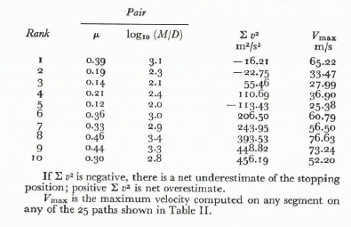
For the ten best fits, M/D has a range defined as 2.0 ≤ log 10(M/D) ≤ 3.4. This range (c. 102 m to 103 m) is consistent with our estimate of M/D using expected M and D values for large avalanches, as derived in our previous section. Moreover, the corresponding maximum velocities are consistent with maximum velocity observations as reviewed by Perla (in press). The interesting feature is that we did not input velocity to arrive at the ranking of Table III, Rather, we have computed from input data of stopping distances that maximum velocity is somewhere in the range 25 ≤ Vmax ≤ 76 m/s for the ten best fits.
The fact that a solution with a relatively high velocity (Vmax = 65 m/s) ranked first is probably not significant because of the wild fluctuation of {µ, M/D} in successive rankings. Quite possibly, a lower velocity solution would rank first on a finer grid; for example Δµ . = 0.001, Δlog10(M/D) = 0.01. In any case, the range of {µ, M/D} cannot be narrowed further without narrowing the range of V max. Unfortunately, definitive velocity data are scarce.
A Uniqueness Problem
Suppose we have field measurements of velocity υ(s) on a path of known geometry, can we compute µ(s) and M/D(s) ? The answer isno, because referring back to Equation (13), we note there are infinitely many combinations of µi and (M/D)i which satisfy the given data V iA, V iB,L i, and 0 i and for the ith segment. In other words, the unfortunate fact is that even with a complete set of velocity measurements from start to stop—measurements that are presently rare and not easy to obtain—we still cannot determine uniquely how μ and M/D vary on a given path. This uniqueness problem, intrinsic to two-parameter models such as {µ, M/D} or Voellmy’s {µ, ξH}, or for that matter any model based on any two terms from Equation (17), is apparently subtle enough not to have been emphasized previous to our paper. It is not difficult to construct an alternative model based on one parameter that can be determined uniquely from velocity data. We return to Equation (8), introduce one generalized parameter for ![]() say G, and we have in place of Equation (12)
say G, and we have in place of Equation (12)

Now, given the same data for the ith segment (ViA, ViB,Li and θi), and assuming (G/M)i is constant for the length of the segment, we obtain the unique value
With enough data it should eventually be possible to correlate G/M with such factors as velocity and slope angle in order to test statistically the υ2 assumption and whether “friction” is actually proportional to normal force (Mg cos θ ).
Conclusions
Voellmy’s model is encumbered by the need to choose a mid-slope reference position for the computation of terminal velocity and run-out distance. Results depend on where the reference is located, however there is usually no firm reason for selecting one reference position in preference to another. To overcome this flaw, we have derived a differential equation which describes the motion of the centre of mass of an avalanche from start to stop down a slope of arbitrary geometry. Numerical solutions depend critically on two parameters: a friction coefficient μ, and a dynamic resistance parameter M/D which is the ratio of avalanche mass M to dynamic drag D. The equation and solutions are analogous to Voellmy’s two-parameter model which assumes an avalanche is an endless fluid. The analogy follows because both theories include a dynamic resistance proportional to Ʋ2
The ranges of µ and M/D (or Voellmy’s µ and ξH) are not presently known to useful precision. It is possible to compute a µ. and M/D that best predict the stopping position of a group of paths, but this is an unstable computation in the sense that widely different pairs of µ and M/D rank closely as predictors of identical stopping positions. More refined estimates of µ and M/D depend on avalanche velocity data in addition to measurements of stopping position.
Even with complete velocity data for a given path, it is not possible to compute uniquely how µ and M/D vary on the given path. This is due to the mathematical redundancy of a two parameter model.
Acknowledgements
Many of the ideas presented here are the result of stimulating discussion and correspondence with Bruno Salm, Hans Gubler, and Marcel de Quervain, Eidg. lnstitut für Schnee- und Lawinenforschung, Davos. We owe additional ideas to correspondence with Bonsak Schieldrop, Industriell Hydro- og Aerodynamikk, Oslo.


