2.1. Experimental set-up

A water jet seeded with particles was studied in the Lagrangian Exploration Module (LEM) at the École Normale Supérieure de Lyon. The vertical water jet is injected with a pump connected to a reservoir into the LEM, a convex regular icosahedral (20-faced polyhedron) tank full of water. A schematic of the set-up is shown in figure 2. The jet is ejected upwards from a round nozzle with a diameter $D = {4}\ {\rm mm}$. At the nozzle exit, the flow rate is $Q \simeq 10^{-4} {{\rm m}}^{3}\ {\rm s}^{-1}$, generating an exit velocity $U_J \simeq {7}\ {\rm m}\ {\rm s}^{-1}$, and, in turn, a Reynolds number based on the nozzle diameter $Re_D = U_JD/\nu \simeq 2.8\times 10^{4}$, with $\nu$ as the water kinematic viscosity. An overflow valve releases the excess water from the top of the tank at the same rate as injection from the nozzle. Experiments are performed at ambient temperature.

Figure 2. Schematic of the experimental set-up. The three high-speed cameras are oriented orthogonal to the brown faces.

The vertical position of the nozzle is chosen to observe a jet sufficiently far from the walls to discount momentum effects from the LEM on the jet (Hussein et al. Reference Hussein, Capp and George1994), and thus a free jet is observed. The interrogation volume spans ${100}\ {\rm mm} \leqslant z \leqslant 180\ {\rm mm}$ ($25 \leqslant z/D \leqslant 45$) with the $z$ axis along the jet axis and $z = 0$ the nozzle exit position. In this region, the jet is self-similar (self-similarity holds for $z \gtrsim 15D$) and the centreline velocity is between 1 and ${2}\ {\rm m}\ {\rm s}^{-1}$.

The particles, seeding the jet during injection, are neutrally buoyant spherical polystyrene tracers with a density $\rho _p = {1060}\ {\rm kg}\ {\rm m}^{-3}$ and a diameter $d_p = {250}\ {\mathrm {\mu }}{\rm m}$. The reservoir is seeded with a mass loading of 0.05 % (reasonable seeding to observe a few hundreds of particles per frame) and an external stirrer maintains homogeneity of the particles. The quiescent water inside the LEM is not seeded, therefore tracked particles are, in principle, only those injected into the measurement volume through the nozzle. In practice, it is unavoidable that a few particles eventually end up being resuspended in the surrounding fluid and reentrained within the jet. This could be caused by several phenomena: the flow rate within the jet is growing with the axial distance due to entrainment and thus part of the core of the jet cannot flow out and remains in the LEM with some tracers; rarely, some particles can be detrained and reentrained later or, in the same way, drift out due to their slight inertia or finite size effect. The main effect is probably that, because between each movie we switch the jet on and off, while nearly all the injected particles are eliminated in the overflow, some particles stay in the LEM when the jet is switched off. The probed flow is therefore almost exclusively tagged by nozzle seeded particles with a minor residual contribution of entrained particles (residual homogeneous seeding). In the following, we will refer to this specific seeding as nozzle seeding. Additional measurements with a homogeneous seeding in the whole volume of the LEM (mass loading of 0.1 %) without nozzle seeding are also realised and will be discussed too. The inlet valve is open some seconds before the recording, in such a way that the jet is stationary but minimal particle recirculation occurs, ensuring a limited pollution of the surrounding fluid with particles or any spurious background flow.

Three high-speed cameras (Phantom V12, Vision Research) mounted with 100 mm macro lenses (Zeiss Milvus) are used to track the particles. The interrogation volume is illuminated in a back-light configuration with three 30 cm square light-emitting diode panels oriented one opposite to each camera. The spatial resolution of each camera is $1280 \times 800$ pixels, creating a measurement volume of around $80\ {\rm mm}\times 100\ {\rm mm}\times 130\ {\rm mm}$. Hence, one pixel corresponds to approximately ${0.1}\ {\rm mm}$. The three cameras are synchronised via transistor–transistor logic (TTL) triggering at a frequency of 6 kHz for 8000 snapshots, resulting in a total record of nearly 1.3 s per run. A total of 50 runs are performed to ensure statistical convergence.

2.2. Particle tracking and post-processing

Lagrangian particle tracking requires three main steps to compute the tracks: particle detection, stereoscopic reconstruction and tracking. A brief description of the method is presented herein (the particle tracking source codes used for the present study are available on request).

1. (i) Particle detection enables the measurement of positions of the centres of the particles in the camera images by using an ad hoc process based on classical methods of image analysis such as non-uniform illumination correction and centroid detection.

2. (ii) Stereoscopic reconstruction aims at finding the particle coordinates in three-dimensional space by combining the two-dimensional views from the three cameras. To achieve this, an accurate calibration is required, allowing the connection of pixel coordinates to real world coordinates. A recent polynomial calibration developed in Machicoane et al. (Reference Machicoane, Aliseda, Volk and Bourgoin2019) and the matching algorithm by Bourgoin & Huisman (Reference Bourgoin and Huisman2020) are used. The maximum tolerance of ray crossing for stereoscopic matching errors (due to experimental noise such as pixel locking and thermal noise of the camera CMOS sensor) is set to ${50}\ {\mathrm {\mu }}{\rm m}$, i.e. one fifth of the particle diameter.

3. (iii) Tracking of the particles through time transforms the cloud of points into trajectories. This is obtained with a classical nearest neighbour approach to initialise tracks and coupled with a predictive tracking based on a linear fit over the five previous positions (Ouellette, Xu & Bodenschatz Reference Ouellette, Xu and Bodenschatz2006; Viggiano et al. Reference Viggiano, Basset, Solovitz, Barois, Gibert, Mordant, Chevillard, Volk, Bourgoin and Cal2021).

Finally, the trajectories are smoothed by convolution with a Gaussian kernel and the velocities are computed by convolving tracks with a first-order derivative Gaussian kernel (Mordant, Crawford & Bodenschatz Reference Mordant, Crawford and Bodenschatz2004). We stress that smoothing does not degrade the temporal resolution for the velocity estimates presented here as the sampling frequency of the cameras (6 kHz) oversamples the dissipation time scale $\tau _\eta$ between 0.3 and 0.8 ms (Viggiano et al. Reference Viggiano, Basset, Solovitz, Barois, Gibert, Mordant, Chevillard, Volk, Bourgoin and Cal2021). Smoothing improves the signal-to-noise ratio of velocity estimates, whose absolute accuracy is estimated (from small-scale Lagrangian increments statistics (Viggiano et al. Reference Viggiano, Basset, Solovitz, Barois, Gibert, Mordant, Chevillard, Volk, Bourgoin and Cal2021)) to be of the order of $10^{-3}\ {\rm m}\ {\rm s}^{-1}$. Considering that the typical axial velocity of the jet on the axis is ${1}\ {\rm m}\ {\rm s}^{-1}$, this accuracy corresponds to a dynamical range of velocity resolution of approximately three orders of magnitude. The corresponding error bars in the mean velocity profiles discussed in this article are therefore of the order of the size of the points in the plots and will be omitted.

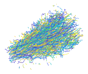
The coordinate basis is adapted by coinciding the $z$ axis with the jet axis and centring it in the $x$ and $y$ directions. Positions and velocities are computed in adapted cylindrical coordinates. A visualisation of tracks is shown in figure 3. It can be noted that most trajectories come from the nozzle (where they are injected) and very few come from the outside and correspond to particles entrained into the jet (visible in figure 3 as radial trajectories towards the jet). The full data set is comprised of $3.5\times 10^{6}$ trajectories longer than or equal to four frames with a mean length of 29 frames, which corresponds to $1.0\times 10^{8}$ particle positions and velocities obtained from 50 independent runs. This amount of statistics ensures sufficient convergence, in spite of the strong axial and radial spatial conditioning we will use (axisymmetry of the configuration allows us to average statistics over the circumferential component). As a consequence, all points of the velocity profiles for the nozzle seeding experiments we will present result from averages taken over several $10^{3}$ or $10^{4}$ points.

Figure 3. A sample of tracks: 14 182 tracks longer than or equal to 50 frames (one colour per trajectory, one film considered). The majority of the particles come from the nozzle, a few of them come from the tank.

A more complete description of the hydraulic and optical set-ups as well as Lagrangian particle tracking and post-processing methods is given in Viggiano et al. (Reference Viggiano, Basset, Solovitz, Barois, Gibert, Mordant, Chevillard, Volk, Bourgoin and Cal2021) which focuses on Lagrangian statistics in the same flow.

3.1. Mean axial velocity

We first recall known properties of the mean axial velocity in the self-similar region far from the nozzle (approximately for $z \gtrsim 15D$ with $D$ the nozzle diameter). We consider the mean centreline velocity $U_0(z) = \langle U \rangle (z,r=0)$, and its half-width $r_{1/2}(z)$ such that $\langle U \rangle (z,r=r_{1/2}(z)) = U_0(z)/2$. Self-similarity enables characterisation of the mean axial velocity by these three relations

(3.1)\begin{equation} U_0(z) = \dfrac{BU_JD}{z-z_0}, \end{equation}

with $U_J$ the jet axial velocity at the nozzle, $z_0$ a virtual origin and $B$ a dimensionless constant (typical values are $z_0 \simeq 4D$ and $B \simeq 5.8$ according to Pope Reference Pope2000; Lipari & Stansby Reference Lipari and Stansby2011)

(3.2)\begin{equation} r_{1/2}(z) = S(z-z_0), \end{equation}

with $S$ a dimensionless constant (typical value is $S \simeq 0.094$ according to Pope Reference Pope2000; Lipari & Stansby Reference Lipari and Stansby2011)

(3.3)\begin{equation} f(\eta) = \dfrac{\langle U \rangle (z,r)}{U_0(z)}, \end{equation}

which is the radial profile in its self-similar form with the dimensionless self-similar coordinate $\eta = r/(z-z_0)$.

The self-similar mean axial velocity profile $f$ must satisfy some constraints: by definition $f(0) = 1$, while $f'(0) = 0$ because $f$ is even and smooth (the prime notation represents the derivative with respect to the self-similar variable $\eta$). It is also expected to decrease towards 0 as $\eta$ increases (i.e. downstream and/or outwards the jet). However, no exact analytical expression is known for $f$. Because the jet and other free shear flows are slender flows, i.e. they do not extend far in the lateral direction and mainly extends in the axial direction, the averaged turbulent boundary-layer equations are the usual theoretical framework for the jet (Schlichting & Gersten Reference Schlichting and Gersten2017). Using these equations as an approximation for the jet dynamics and assuming a constant (uniform) turbulent viscosity (Pope Reference Pope2000; Schlichting & Gersten Reference Schlichting and Gersten2017) (which will be further discussed in § 5 and Appendix B), an approximate analytical expression can be calculated for $f$ leading to a squared Lorentzian function

(3.4)\begin{equation} f(\eta) \simeq (1+A\eta^{2})^{{-}2}, \end{equation}

with $A = (\sqrt {2}-1)/S^{2}$. Experimentally, the squared Lorentzian profile is found to reasonably hold near the jet centreline ($\eta \lesssim 0.15$), but to deviate from the measured profile at larger $\eta$. This indicates that an accurate description of the self-similar mean profile must account for the non-uniformity of the turbulent viscosity, which requires to be experimentally determined. It is empirically found that an improved global fit of $f$ is obtained using a Gaussian function (So & Hwang Reference So and Hwang1986)

(3.5)\begin{equation} f(\eta) \simeq {\rm e}^{{-}A\eta^{2}}, \end{equation}

with $A = \log (2)/S^{2}$.

The estimate of the mean field $\langle U_\varphi \rangle$ (based on experimental trajectories with a nozzle seeding) is performed in cylindrical coordinates $(z,r,\theta )$ and then averaged over $\theta$ (due to axisymmetry) leading to statistics in the two-dimensional space $(r,z)$. In practice, we bin space in $r$ and $z$ every 0.5 mm and compute the mean axial velocity of the particles inside each bin. For the self-similar profiles, we bin in $\eta$ by steps of 0.01. Figure 4 shows the radial profiles of the mean axial velocity $\langle U_\varphi \rangle (z,r)$ at different downstream positions $z$, the axial evolution of the mean centreline velocity $U_{0\varphi }(z)$ and of the half-width $r_{1/2\varphi }(z)$ and the self-similar profile $f_\varphi (\eta )$ measured in our experiment when probing solely nozzle seeded particles.

Figure 4. Characterisation of the mean axial velocity field $\langle U_\varphi \rangle$ based on trajectories with a nozzle seeding. (a) Radial profiles of the mean axial velocity $\langle U_\varphi \rangle$ (crosses: experimental points, solid lines: Gaussian fit). (b) Mean centreline velocity $U_{0\varphi }(z)$ (crosses: experimental points, solid line: fit (3.1)). (c) Half-width $r_{1/2\varphi }(z)$ (crosses: experimental points, solid line: fit (3.2)). (d) Self-similar profiles $f_\varphi (\eta )$ (3.3) (crosses: experimental points, solid line: fit (3.5)).

When comparing the nozzle seeded particle measurements with the classical Eulerian relations given by (3.1), (3.2) and (3.3), we observe an excellent agreement. In particular, self-similarity is very well satisfied, with a Gaussian self-similar profile $f_\varphi$ and fitting parameters $B_\varphi = 5.3$ and $S_\varphi = 0.105$ ($A_\varphi = 63$), which are consistent with those classically determined for the global Eulerian jet dynamics (Pope Reference Pope2000; Lipari & Stansby Reference Lipari and Stansby2011). The value of $S_\varphi$ is found to be slightly larger than the values reported in Eulerian measurements which usually span between 0.09 and 0.10 (Lipari & Stansby Reference Lipari and Stansby2011), suggesting that the nozzle seeded particle profile is slightly wider than the actual Eulerian profile. Despite this small difference, we will consider in the sequel that $f \simeq f_\varphi$.

This first observation suggests that the axial dynamics of nozzle seeded particles accurately represents the global axial Eulerian dynamics, even if entrained particles are not probed. This will be further qualitatively discussed in the next subsection and quantitatively justified in § 5. We will see in the next subsection that, on the contrary, entrained particles play a crucial role in the mean radial velocity profile.

3.2. Mean radial velocity – an incompressibility paradox

We now perform the same study for the mean radial velocity. As previously done with the mean axial velocity $\langle U \rangle$, we can define a self-similar profile for the mean radial velocity $\langle V \rangle$

(3.6)\begin{equation} g(\eta) = \dfrac{\langle V \rangle (z,r)}{U_0(z)}. \end{equation}

Interestingly, in an incompressible jet, $\langle U \rangle$ and $\langle V \rangle$ are linked through the continuity equation

(3.7)\begin{equation} \boldsymbol{\nabla}\boldsymbol{\cdot}\langle \boldsymbol{U} \rangle = 0, \end{equation}

where $\langle \boldsymbol {U} \rangle = \langle U \rangle \boldsymbol {e_z} + \langle V \rangle \boldsymbol {e_r}$. Combining (3.1) and definitions (3.3) and (3.6), the continuity equation (3.7) can be rewritten as (Pope Reference Pope2000)

(3.8)\begin{equation} \eta (\eta f(\eta))' = (\eta g(\eta))', \end{equation}

which can be integrated to obtain the following general relation between the self-similar mean radial and axial profiles for the global Eulerian dynamics of an incompressible free round jet:

(3.9)\begin{equation} g(\eta) = \eta f(\eta) - \dfrac{1}{\eta} \int_0^{\eta} x f(x) \,\mathrm{d} x. \end{equation}

Knowing that $f(0) = 1$ and $f'(0) = 0$, we deduce that $g(0) = 0$, $g'(0) = 1/2$ and ${g''(0) = 0}$. Using the empirical Gaussian approximation (3.5) for $f$, (3.9) gives the following approximated expression for $g$:

(3.10)\begin{equation} g(\eta) \simeq \eta {\rm e}^{{-}A\eta^{2}} - \dfrac{1-{\rm e}^{{-}A\eta^{2}}}{2A\eta}. \end{equation}

Figure 5 presents the experimental mean radial velocity profile $g_\varphi (\eta )$ for the nozzle seeding case (obtained as for the axial velocity, binning $z$ in steps of 0.5 mm and $\eta$ in steps of 0.02), which is compared with the self-similar profile $g(\eta )$ (3.10) expected for $\langle V \rangle$ from the previous incompressibility considerations for the global Eulerian profile. It can be observed that, although the measured profiles of $g_\varphi$ do hold self-similarity, they strongly deviate from the expected self-similar incompressible profile for the global jet $g$. More specifically, three points can be highlighted: (i) the amplitude of the measured maximums of $g_\varphi$ is twice that of the expected incompressible profile $g$, (ii) the measured profiles cross zero at a much higher value of $\eta$ and (iii) the slope at the origin ($\eta = 0$) of the measured self-similar profile is 1 instead of 1/2.

Figure 5. Self-similar profiles $g_\varphi (\eta )$ (3.6) for a nozzle seeding (crosses: experimental points, solid line: fit (3.10) with $A_\varphi = 63$ previously found for $f_\varphi (\eta )$).

Overall, contrary to the mean axial velocity profile which is essentially indistinguishable between the nozzle seeding case and the global Eulerian field ($f_\varphi \simeq f$), the mean radial velocity profile is strongly affected by the nozzle seeding up to the core of the jet ($g_\varphi \neq g$). Since the radial and axial velocity profiles are classically linked by simple incompressibility considerations (as just discussed), and considering that the jet under investigation does operate in incompressible conditions, this discrepancy may appear at first sight as a paradox.

In order to rule out any possible experimental error as the origin of the major difference observed between the measured profile with a nozzle seeding $g_\varphi$ and the expected global incompressible profile $g$, we performed experiments with an actual homogeneous seeding in the whole volume of the tank. The measured radial profile $g(\eta )$, shown in figure 6, accurately matches the expected incompressible profile (3.10). Some discrepancy can be observed for $\eta \gtrsim 0.2$, which can be attributed to the fact that $f$ is less well fitted by a Gaussian function as it decreases towards zero. Moreover, with this homogeneous seeding, we find $S = 0.094$ which is a usual value for $S$ (Lipari & Stansby Reference Lipari and Stansby2011).

Figure 6. Self-similar profiles $g(\eta )$ for a homogeneous seeding in the whole volume of the LEM without nozzle seeding (crosses: experimental points, solid line: fit (3.10) with $A = 79$).

This therefore confirms that, when homogeneous seeding is used, global mean radial and axial velocity profiles $f$ and $g$ are correctly retrieved by the particle tracking measurements and found to be consistently related by the incompressibility constraint leading to (3.9), while for nozzle seeding, $f_\varphi \simeq f$ but $g_\varphi$ truly deviates from $g$ and appears to not comply with the incompressibility constrain. As a matter of fact, such an impact on the seeding properties on the retrieved velocity profiles is well known by experimentalists using a particle-based metrology (as stated in the introduction such as particle image velocimetry or laser Doppler velocimetry). Martins et al. (Reference Martins, Kirchmann, Kronenburg and Beyrau2021) for instance report similar observations for particle image velocimetry in an annular jet: axial velocity profiles are almost indistinguishable between the two seedings while radial velocity profiles strongly deviate. Such deviation is usually addressed simply in terms of an experimental bias to be mitigated, but no quantitative physical explanation has been proposed. Section 4 presents a simple theoretical explanation (based on mass conservation and self-similarity properties of the jet) of this apparent paradox. The proposed theory quantitatively describes the experimental observations through an effective compressibility of the velocity field associated with nozzle seeded particles. The physical origin of this effective compressibility relies on the role played by entrained particles, not accounted for when only nozzle seeded particles are tracked.

Before presenting these theoretical developments, we briefly discuss the qualitative reasons of why nozzle seeding (compared with homogeneous seeding) may strongly impact the radial profile $g$ and not the axial profile $f$. The source of momentum in the jet is the nozzle injection, which provides primarily axial momentum. Entrained particles, which are captured in the jet by the inward transverse pressure gradient, are on the contrary the main source of radial momentum. As they penetrate into the jet, entrained fluid parcels eventually acquire an axial momentum, transferred from the nozzle seeded fluid parcels, which in turn lose axial momentum, which results in the streamwise decay of the jet. In the final steady state both the nozzle and entrained fluid parcels eventually equilibrate to the same axial velocity, with almost indistinguishable profiles. On the contrary, the radial velocity is expected to behave radically differently for nozzle and entrained particles. Indeed, particles entrained from outside to inside the jet acquire a negative radial velocity to reach the core of the jet and therefore contribute negatively to the global radial velocity profile $g$. As they do so, mass and momentum conservation require fluid parcels from the core of the jet to move outwards, with a positive radial contribution to $g$. Therefore, when a homogeneous seeding is considered, the combination of these two contributions (outward spreading and inward entrainment) eventually leads to the global radial profile $g$ (see figure 6), where spreading dominates in the centre ($g(\eta ) > 0$ for $\eta < 0.13$) and entrainment dominates on the sides ($g(\eta ) <0$ for $\eta > 0.13$). When only nozzle seeded particles are tagged, the inward contribution of entrained particles is not accounted in $g_\varphi$. As a consequence, an overall hindering of the negative radial contribution associated with those particles is expected, leading to a higher and mostly positive profile for $g_\varphi$, which therefore considerably deviates from the global radial profile $g$ as experimentally measured (see figure 5).

We present in the next section a simple theoretical and quantitative justification for the deviation between $g$ and $g_\varphi$, based on mass conservation and self-similarity, explaining the apparent compressibility of $g_\varphi$ and explicitly giving the associated contribution of entrainment to the global incompressible radial velocity profile $g$.

4.1. Nozzle seeding model

To account for effective compressibility and compute $g_\varphi$, we propose to generalise the classical approach relating mean radial and axial velocity profiles through incompressibility, in order to account for the inhomogeneity of the concentration field (itself due to the inhomogeneous seeding).

We denote by $\varphi (z,r,\theta,t)$ the instantaneous concentration field of nozzle seeded tracers. As we did for the mean axial and radial velocities, we consider the mean concentration field $\langle \varphi \rangle (z,r)$. The continuity equation for the mean concentration field $\langle \varphi \rangle$ and the mean velocity field $\langle \boldsymbol {U}_{\boldsymbol {\varphi }}\rangle$ imposes that

(4.1)\begin{equation} \boldsymbol{\nabla}\boldsymbol{\cdot}(\langle \varphi \rangle \langle \boldsymbol{U}_{\boldsymbol{\varphi}}\rangle) = 0. \end{equation}

Note that, because by definition $\boldsymbol {U}_{\boldsymbol {\varphi }}$ is exactly the advection velocity of the nozzle seeded tracers (not including any eventually unknown random velocity perturbation, $\boldsymbol {U}_{\boldsymbol {\varphi }}$ is not an Eulerian field), the continuity equation as written above for the mean (concentration and velocity) fields is exact, as there is no additional diffusion term associated with the transport of the tracers by the unperturbed advection velocity $\boldsymbol {U}_{\boldsymbol {\varphi }}$. Note also that, for a homogeneous seeding (i.e. $\langle \varphi \rangle$ independent of all spatial coordinates), (4.1) naturally reduces to the classical incompressible relation $\boldsymbol {\nabla } \boldsymbol {\cdot } \langle \boldsymbol {U}_{\boldsymbol {\varphi }} \rangle = 0$, which, however, does not hold when $\langle \varphi \rangle$ is inhomogeneous, as for the case of nozzle seeded tracers investigated here.

To solve (4.1), we first characterise the mean concentration field $\langle \varphi \rangle (z,r)$. Figure 7 shows the main properties of $\langle \varphi \rangle$: the mean centreline concentration $\varphi _0(z)$ evolves as $1/(z-z_0)$ and we can define a self-similar profile

(4.2)\begin{equation} \varPhi(\eta) = \dfrac{\langle \varphi \rangle (z,r)}{\varphi_0(z)}, \end{equation}

with $\varphi _0(z) \propto 1/(z-z_0)$. The fact that $\langle \varphi \rangle$ evolves as $\langle U \rangle$ can be justified by the behaviour of a conserved passive scalar in a jet. Actually, it is known that, because the boundary-layer equations for the mean axial velocity $\langle U \rangle$ and a scalar field $\langle \varphi \rangle$ are similar, a conserved passive scalar scales with $z$ in the same way as the mean axial velocity does, and the self-similar profile is similar, usually wider (see Pope Reference Pope2000). For the present concentration field, the profiles of $\varPhi$ are wider than those of $f$, this difference of width and also the shape of $\varPhi$ will be discussed in the next section.

Figure 7. Characterisation of the mean concentration field $\langle \varphi \rangle$. (a) Centreline concentration $\varphi _0(z)$ (crosses: experimental points, solid line: fit in $1/(z-z_0)$). Here, $\varphi _0$ is the sum of the concentrations from all films at all time steps, which explains the high values of $\varphi _0$, but only the relative evolution along $z$ is relevant. (b) Self-similar profiles $\varPhi (\eta )$ (4.2) (crosses: experimental points, dashed line: $f_\varphi (\eta )$ previously measured). The profiles of $\varPhi (\eta )$ are wider than those of $f_\varphi (\eta )$.

From (4.1) and definition (4.2), we infer that self-similar profiles of mean concentration, radial and axial velocity of nozzle seeded particles must satisfy the following relation:

(4.3)\begin{equation} \varPhi(\eta) [(\eta g_\varphi(\eta))' - \eta (\eta f_\varphi(\eta))'] + \eta [g_\varphi(\eta) \varPhi'(\eta) - f_\varphi(\eta)(\eta \varPhi(\eta))'] = 0, \end{equation}

which simplifies to

(4.4)\begin{equation} g_\varphi(\eta) = \eta f_\varphi(\eta). \end{equation}

The details of this calculation are given in Appendix A. It can be noticed that this result does not depend on the exact shape of $\varPhi$: only the dependence of $\varphi _0(z)$ in $1/(z-z_0)$ and the self-similarity of $\varPhi (\eta )$ are required.

Interestingly, the solution for the effectively compressible fields in the case of the nozzle seeding turns out to be somehow simpler than the global incompressible case, as it does not carry the additional term

(4.5)\begin{equation} \zeta(\eta) ={-} \dfrac{1}{\eta} \int_0^{\eta} x f(x) \,\mathrm{d} x. \end{equation}

Going back to (3.9) and considering $f = f_\varphi$, we can see that the global mean radial velocity profile (accounting for both nozzle seeded and entrained particles) can be written as the sum of the profile of the nozzle seeded particles alone and this $\zeta$ term

(4.6)\begin{equation} g = g_\varphi + \zeta. \end{equation}

The $\zeta$ contribution can therefore be interpreted as the effect of entrained particles on the global mean radial velocity profile of the jet. Its negative sign naturally reflects the inward flux of particles due to entrainment. Therefore, we will refer to $\zeta$ as the entrainment term.

4.2. Experimental validation

A first interesting property of (4.4) is that, as $f_\varphi (0) = 1$ by definition, then $g'_\varphi (0) = 1$. This is agreement with the experimental slope of 1 observed in figure 5 for $g_\varphi (\eta )$ at $\eta = 0$. Considering a Gaussian function for $f_\varphi$, which was found in a previous section to reasonably matches the experimental measurements, we have the expression

(4.7)\begin{equation} g_\varphi(\eta) \simeq \eta {\rm e}^{{-}A\eta^{2}}. \end{equation}

Figure 8 compares this expression with the experimental profiles for $g_\varphi$, showing a much better agreement than the usual expression tested in figure 5 for the global profile $g$, with not only the expected slope at the origin, but also a reasonable overall shape, at least up to $\eta \lesssim 0.2$. The main noticeable difference concerns the negative part of the experimental $g_\varphi$ for the largest values of $\eta$, while the prediction given by (4.7) remains positive. This negative part reflects the presence of an inward radial velocity in the outer regions of the jet. This is very likely to be attributed to the presence of a few remaining particles in the ambient fluid (not injected at the nozzle) being entrained into the core of the jet. As a consequence, if some entrained particles are indeed tagged, it is expected that the radial profile measured is not exactly $g_\varphi$ but also carries some contribution due to the negative entrainment term $\zeta$. These few entrained particles with negative radial velocity may also explain the slight overestimation of the maximum of the radial velocity profile prediction compared with the experimental data. Despite this bias, experimental data globally support the validity of relation (4.7) and hence of (4.4).

Figure 8. Self-similar profiles $g_\varphi (\eta )$ for a nozzle seeding (crosses: experimental points, solid line: fit (4.7) with $A_\varphi = 63$ previously found for $f_\varphi (\eta )$). This is the same figure as figure 5 but with the new fit (4.7).

The validity of these relations is also tested on a separate data set from an independent experiment, using similar methods at the Université Grenoble Alpes with a self-similar round free air jet seeded with neutrally buoyant millimetric soap bubbles inflated with helium ($D = {2.25}\ {\rm cm}$, $U_J \simeq {25}\ {\rm m}\ {\rm s}^{-1}$, $Re_D \simeq 3.7\times 10^{4}$, $d_p = {2.5}\ {\rm mm}$). The advantage of this set-up is that the jet blows in a very large room, and that helium filled soap bubbles have a finite life time, so that experiments can be run with the warranty that no spurious particles remain in the ambient fluid surrounding the jet. Mean axial and radial velocity profiles for this experiment are represented in figure 9. The statistical convergence of this new data set is not as accurate as for the water experiment and the accessible measurement volume does not allow us to explore values of $\eta$ above 0.3. However, it can still be seen that no negative values of $g_\varphi$ are measured and that the maximum of the experimental profile matches very well the prediction in that case where entrained particles have been totally avoided. The slight difference in the profiles between the air and water experiments (for instance the maximum of $g_\varphi$ in air is a bit larger than in water) are related to a slightly different value of the fitting parameter $A_\varphi$ of the Gaussian fit for the mean axial velocity profile $f_\varphi$, which could be linked to different geometries of the set-up or to the total absence of entrained particles in the air jet.

Figure 9. Characterisation of the mean velocity field for an air jet seeded through the nozzle with neutrally buoyant soap bubbles. Self-similar profiles for mean (a) axial and (b) radial velocities (crosses: experimental points, solid lines: fits (3.5) and (4.7) with $A_\varphi = 42$).

5.1. Advection–diffusion equation with turbulent diffusivity $K_T$

We consider that the tracers are, on the one hand, advected by the mean flow, and on the other hand, spread by turbulence. Modelling this turbulent process as diffusive, we write

(5.1)\begin{equation} \boldsymbol{\nabla}\boldsymbol{\cdot}(\langle \varphi \rangle \langle \boldsymbol{U} \rangle - K_T \boldsymbol{\nabla} \langle \varphi \rangle) = 0, \end{equation}

with $K_T$ the turbulent diffusivity. Equation (5.1) is the same as (4.1) with the relation between $\langle \boldsymbol {U} \rangle$ and $\langle \boldsymbol {U}_{\boldsymbol {\varphi }} \rangle$

(5.2)\begin{equation} \langle \boldsymbol{U}_{\boldsymbol{\varphi}} \rangle = \langle \boldsymbol{U} \rangle - K_T \dfrac{\boldsymbol{\nabla} \langle \varphi \rangle}{\langle \varphi \rangle}, \end{equation}

where $\langle \boldsymbol {U}_{\boldsymbol {d}} \rangle = -K_T ({\boldsymbol {\nabla } \langle \varphi \rangle }/{\langle \varphi \rangle }$ represents the aforementioned diffusive contribution.

With previous definitions for the self-similar mean axial and radial velocity fields and mean concentration profile, and considering the decay law for the centreline velocity from (3.1) ($U_0(z) = BU_JD/(z-z_0$)), (5.2) leads to two expressions for the self-similar mean axial and radial velocity profiles of the spreading particles

(5.3)\begin{gather} f_\varphi(\eta) = f(\eta) + \dfrac{K_T(\eta)}{BU_JD} \left[1+\eta\dfrac{\varPhi'(\eta)}{\varPhi(\eta)}\right], \end{gather}

(5.4)\begin{gather}g_\varphi(\eta) = g(\eta) - \dfrac{K_T(\eta)}{BU_JD} \dfrac{\varPhi'(\eta)}{\varPhi(\eta)}, \end{gather}

where the first term in the right-hand side of both expressions accounts for advection and the second for diffusion. At this stage, (5.3) and (5.4) are nothing but mathematical expressions reflecting the a priori advection/diffusion decomposition of the particle velocity in (5.2). To be physically relevant, they have to be consistent with the experimental observations and the results of the mass conservation presented in previous sections for $f$, $g$, $f_\varphi$ and $g_\varphi$.

First, our experiments show that $f \simeq f_\varphi$. To be consistent with (5.3), this requires the second term of this relation to be negligible compared with $f$. Experimental measurements of the turbulent diffusivity $K_T$ and of the self-similar mean concentration field $\varPhi$ (presented in the following) confirm the validity of this approximation (this term has the same order of magnitude as $g$, thus it is more than one order of magnitude smaller than $f$).

Second, to be consistent with (4.6), (5.4) implies that

(5.5)\begin{equation} K_T(\eta) ={-} BU_JD \dfrac{\varPhi(\eta)}{\varPhi'(\eta)} \dfrac{1}{\eta} \int_0^{\eta} x f(x) \,\mathrm{d} x. \end{equation}

Thus, the turbulent diffusivity $K_T(\eta )$ is a self-similar quantity dependent on space and expression (5.5) gives a practical relation to estimate it from the knowledge of simple mean field quantities (namely mean concentration and mean axial velocity profiles) which are easily measurable. This contrasts both with classical simplistic approaches assuming a constant turbulent diffusivity and with the usual fundamental definition of turbulent diffusivity, based on the cross-correlation between velocity and concentration fluctuations (Pope Reference Pope2000).

The parameter $K_T(\eta )$ as given by relation (5.5) is a dimensional quantity (with units ${\rm m}^{2}\ {\rm s}^{-1}$). Similarly to all other self-similar quantities characterising the jet, and as it is done for turbulent viscosity, a dimensionless turbulent diffusivity $\hat {K}_T$ can be defined

(5.6)\begin{equation} \hat{K}_T(\eta) = K_T(\eta) / (U_0(z)r_{1/2}(z)) ={-} \dfrac{1}{S} \dfrac{\varPhi(\eta)}{\varPhi'(\eta)} \dfrac{1}{\eta} \int_0^{\eta} x f(x) \,\mathrm{d} x, \end{equation}

which can ultimately be rewritten as

(5.7)\begin{equation} \hat{K}_T(\eta) = \frac{\zeta(\eta)}{S\chi(\eta)}, \end{equation}

where $\zeta (\eta ) = -({1}/{\eta })\int _0^{\eta } x f(x) \,\mathrm {d} x$ has already been defined in (4.5) and shown to be associated with entrainment, $\chi (\eta )= \varPhi '(\eta )/\varPhi (\eta )$ characterises the persistent inhomogeneity of the seeding and can be interpreted as a compressibility factor associated with the flow of nozzle seeded particles and $S = \tan (\delta ) \simeq \delta$ with $\delta$ the semi-opening angle of the jet cone based on $r_{1/2}$.

Overall, relation (5.7) synthesises the connection between the a priori advection/diffusion mathematical decomposition of particle velocity and the physical considerations of mass conservation developed in previous sections by connecting the turbulent diffusivity $K_T$ to (i) entrainment (via $\zeta$), (ii) apparent compressibility of the dispersing phase (via $\chi$) and (iii) global spreading of the jet (via $S$). Note that a conceptually similar connection between effective diffusivity and effective compressibility has been proposed in the context of mixing in linear flows (Raynal et al. Reference Raynal, Bourgoin, Cottin-Bizonne, Ybert and Volk2018).

5.2. Turbulent diffusivity and turbulent viscosity

The turbulent diffusivity $K_T$ and the turbulent viscosity $\nu _T$ are both effective transport coefficients defined in the framework of a mean field description (transport of mass for the first and of momentum for the second). They model the average contribution of small-scale turbulence via cross-correlation terms of fluctuating quantities ($\langle u\varphi ' \rangle$ for $K_T$ and $\langle uv \rangle$ for $\nu _T$, with fluctuating quantities $u = U - \langle U \rangle$, $v = V - \langle V \rangle$ and $\varphi ' = \varphi - \langle \varphi \rangle$ Pope Reference Pope2000). This formal analogy between $K_T$ and $\nu _T$, together with the importance of $\nu _T$ for practical numerical modelling strategies (such as Reynolds-averaged Navier–Stokes (RANS) approaches) and the simplicity of the relations established in the previous subsection allowing the estimation of $K_T$ from simple measurements of mean field quantities, motivate us to further extend previous considerations (connecting turbulent diffusivity to entrainment and mass conservation) in order to revisit formal links between turbulent diffusivity and turbulent viscosity.

The relation between $K_T$ and $\nu _T$ is commonly written in terms of the turbulent Prandtl number, $\sigma _T = \nu _T/K_T$, which compares the efficiency of momentum and mass transport. Several studies have investigated the turbulent Prandtl number by studying for instance the turbulent transport of conserved passive scalars such as temperature (Corrsin & Uberoi Reference Corrsin and Uberoi1950; Chevray & Tutu Reference Chevray and Tutu1978; Chua & Antonia Reference Chua and Antonia1990; Ezzamel, Salizzoni & Hunt Reference Ezzamel, Salizzoni and Hunt2015) or concentration of chemical species (Papanicolaou & List Reference Papanicolaou and List1988; Dowling & Dimotakis Reference Dowling and Dimotakis1990; Panchapakesan & Lumley Reference Panchapakesan and Lumley1993b; Lemoine, Wolff & Lebouche Reference Lemoine, Wolff and Lebouche1996; Chang & Cowen Reference Chang and Cowen2002), leading to values of $\sigma _T$ of the order of unity (experimental values around 0.7 are usually reported). However, there is no consensus about how $\sigma _T$ exactly depends on space and none of these studies explicitly address the question of a possible formal connection with simple mean field quantities.

5.2.1. Uniform $\sigma _T$

In the case where $\sigma _T$ is assumed to be uniform (independent of space), it can be shown from the turbulent boundary-layer equations (see Schlichting & Gersten Reference Schlichting and Gersten2017) that

(5.8)\begin{equation} \varPhi(\eta) = f(\eta)^{\sigma_T} \quad \textrm{or equivalently} \quad \sigma_T = \frac{\log\varPhi}{\log f}. \end{equation}

This relation combined with the expression of $K_T$ (5.6) leads to the following expression for the turbulent viscosity:

(5.9)\begin{equation} \hat{\nu}_T(\eta) ={-} \dfrac{1}{S} \dfrac{f(\eta)}{f'(\eta)} \dfrac{1}{\eta} \int_0^{\eta} x f(x) \,\mathrm{d} x. \end{equation}

As for $K_T$, $\nu _T$ can be inferred by simply measuring the profile $f$ of mean axial velocity and is analytically connected to the entrainment term $\zeta$.

If we consider for instance a squared Lorentzian approximation (3.4) for $f$, expression (5.9) simplifies to a constant value

(5.10)\begin{equation} \hat{\nu}_T^{Lorentz} = \dfrac{S}{8(\sqrt{2}-1)}. \end{equation}

This is expected, as the squared Lorentzian profile for $f$ is known to be the exact solution of the turbulent boundary-layer equations for a constant turbulent viscosity (Pope Reference Pope2000) (which is experimentally reasonable for $\eta \lesssim 0.15$). In addition, the relation found in (5.10) between $\hat {\nu }_T$ and $S$ coincides with the classical result when solving the boundary-layer equations for a constant turbulent viscosity.

Expression (5.9) is, however, more general and remains valid beyond the constant turbulent viscosity approximation (it still requires the turbulent Prandtl number to be constant, however). In particular, if the Gaussian approximation (3.5) is considered for $f(\eta )$ (which is empirically known to better match the experimental self-similar profiles), the following space-dependent profile is retrieved for the turbulent viscosity:

(5.11)\begin{equation} \hat{\nu}_T^{Gauss}(\eta) = \dfrac{S}{4\log(2)} \dfrac{1-{\rm e}^{{-}A\eta^{2}}}{A\eta^{2}}. \end{equation}

This result is not new, and has been previously derived by So & Hwang (Reference So and Hwang1986), who propose a generalisation of the solution of the turbulent boundary-layer equations for a non-uniform turbulent viscosity. By considering different experimental functions used to fit $f$, they argue that the Gaussian function is the best one to fit experimental profiles of $f$ and they analytically determine the expression for $\hat {\nu }_T$ for a Gaussian function, which is exactly the same as (5.11).

At this point, we have therefore shown that formula (5.8) (valid in the case of a uniform turbulent Prandtl number $\sigma _T$) allows us to extend the connection established in the previous subsection between turbulent diffusivity and entrainment, to turbulent viscosity with relation (5.9). Besides, this quite general relation is found in agreement with previous derivations, based on boundary-layer equations, for squared Lorentzian and Gaussian mean axial velocity profiles. The next subsection generalises formula (5.8) to the case of non-uniform $\sigma _T$.

5.2.2. Generalisation to non-uniform $\sigma _T$

In Appendix B, we show that the general equations (5.6) and (5.9) for $\hat {K}_T(\eta )$ and $\hat {\nu }_T(\eta )$, respectively, relating the self-similar profiles of turbulent diffusivity and turbulent viscosity to the self-similar profiles of mean concentration $\varPhi$, mean axial velocity $f$ and entrainment term $\zeta$, are actually the general solutions of the boundary-layer equations.

Furthermore, we also conclude that these two relations remain valid even if the turbulent Prandtl number $\sigma _T(\eta )$ is not constant, and we show that

(5.12)\begin{equation} \sigma_T(\eta) = \dfrac{\varPhi'(\eta)}{\varPhi(\eta)} \dfrac{f(\eta)}{f'(\eta)}, \end{equation}

is a generalisation of formula (5.8).

Altogether, beyond the conceptual interest of relating effective transport coefficients in the jet to the entrainment process, relations (5.6), (5.9) and (5.12) are of great practical interest as they allow determination of the spatial profiles of turbulent diffusivity, turbulent viscosity and turbulent Prandtl number from the simple measurements of the mean axial velocity profile and the mean concentration profile without requiring the measurement of second-order correlations.

In the next subsection, we apply these relations to experimental measurements.

5.3. Experimental determination of $K_T$, $\nu _T$ and $\sigma _T$

According to (5.6), (5.9) and (5.12), $\hat {K}_T$, $\hat {\nu }_T$ and $\sigma _T$ can be experimentally determined from the sole knowledge of the profiles of $f$ and $\varPhi$ (besides, only $f$ is required to determine $\hat {\nu }_T$). As these relations include the derivatives of $f$ and $\varPhi$, instead of using the raw experimental profiles, it is useful to consider functional fits of these, which can be more easily manipulated.

1. (i) As already discussed, and as can be observed in figure 4(d), $f$ is reasonably fitted by a Gaussian function. However, for a better accuracy, we use the fitting function $f(\eta ) = {\rm e}^{-a\eta ^{2}}(1+c_2\eta ^{2}+c_4\eta ^{4})$ introduced by Hussein et al. (Reference Hussein, Capp and George1994) to fit their experimental measurement of $f(\eta )$ (they also use similar functions to fit the Reynolds stresses). This Gaussian function corrected by a polynomial, although less practical, is closer to the experimental points and leads to a more accurate estimate, in particular, of the derivative $f'(\eta )$ which appears in the formula (5.9) for the turbulent viscosity. The polynomial correction has a minor impact on the estimate of the integral entrainment term $\zeta$.

2. (ii) As can be observed in figure 11, the concentration profile $\varPhi (\eta )$ is broader than a Gaussian function for small values of $\eta$ (typically $\eta <0.1$) and steeper than a Gaussian function for large values of $\eta$. We empirically find that a better function to fit $\varPhi (\eta )$ is

   (5.13)\begin{equation} \varPhi(\eta) = \dfrac{\operatorname{erf}((\eta+a)/b)-\operatorname{erf}((\eta-a)/b)}{2\operatorname{erf}(a/b)}, \end{equation}
   (green line in figure 11, to be compared with the Gaussian fit in light blue) where $\operatorname {erf}(x) = 2/\sqrt {{\rm \pi} } \int _0^{x} {\rm e}^{-t^{2}} \,\mathrm {d}t$ is the error function and $a$ and $b$ the parameters of the fit (here $a = 0.126$ and $b = 0.102$).

Figure 11. Self-similar profiles $\varPhi (\eta )$ (crosses: experimental points, solid lines: fit (5.13) and Gaussian fit with $A_\varPhi = 39$). This is the same figure as figure 7(b) but with the new fit (5.13).

5.3.1. Determination of $K_T$

Based on these fits for $f$ and $\varPhi$, we compute the experimental profiles of $\hat {K}_T(\eta )$ from (5.6), which are shown in figure 12. Profiles are obtained for measurements at different streamwise distances from the nozzle between $z = {100}\ {\rm mm}$ and $z = {180}\ {\rm mm}$. The solid line is the median value for all $z$ positions along the axis, and the coloured zone between the two dashed lines comprises 70 % of the measured values. The profile of $\hat {K}_T$ based on a Gaussian fit of $\varPhi$ is also represented for comparison, showing that small differences between the two fitting functions for $\varPhi$ lead to large differences fin the estimate of $\hat {K}_T$. A good determination of the profile of $\hat {K}_T(\eta )$ therefore requires an accurate measurement of $\varPhi (\eta )$. Figure 12 indicates that the sensitivity to the fit is particularly crucial near the centreline. This can be rationalised from (5.6), from which it can be shown that $\hat {K}_T(0) = -1/(2S\varPhi ''(0))$: the centreline value of $\hat {K}_T(\eta )$ is related to the curvature at the origin of $\varPhi (\eta )$. This explains the underestimate of $\hat {K}_T(0)$ from the Gaussian fit, which is narrower than the error function fit (5.13). It also explains the higher variability of the estimate of $\hat {K}_T$ from the error function fit near the centreline when data from all axial distances $z$ are considered. Indeed, figure 11 shows that, although very good, self-similarity is not perfect within the accessible range of distance from nozzle ($z/D \leqslant 45$). In particular, a mild variation of the curvature at the origin of $\varPhi (\eta )$ measured at different downstream distances $z$ can be seen. This sensitivity to small deviations from self-similarity becomes, however, marginal away from the centreline. Overall, and in spite imperfect self-similarity effects near the centreline (which can be expected to be improved in future studies exploring distances beyond $z/D > 45$), figure 12 shows that a reasonable profile of $\hat {K}_T$ can indeed be retrieved from (5.6) only requiring the determination of mean concentration and axial velocity profiles. Few of such measurements of radial inhomogeneity of turbulent diffusivity are available in the literature, mainly due to the complexity of requiring simultaneous measurements of velocity and scalar fluctuations, as classical estimates are based on velocity–scalar cross-correlations. The profile of $\hat {K}_T$ in figure 12 is in good agreement with such previous measurements in round free jets (Chua & Antonia Reference Chua and Antonia1990; Lemoine et al. Reference Lemoine, Wolff and Lebouche1996; Chang & Cowen Reference Chang and Cowen2002).

Figure 12. Self-similar profile $\hat {K}_T(\eta )$ based on two fits of $\varPhi$ (solid lines: median values, coloured zones limited by dashed lines: 70 % of the measured values).

5.3.2. Determination of $\nu _T$

Similarly to $\hat {K}_T$, the turbulent viscosity $\hat {\nu }_T$ can be estimated from (5.9) knowing the mean axial velocity profile $f$. Figure 13(a) shows the retrieved profile of the turbulent viscosity. As for the turbulent diffusivity, estimates of $\hat {\nu }_T$ are obtained at various downstream locations $z$. The solid line represents the median value for all $z$ locations, and the coloured zone within the dashed lines comprises 70 % of all measurements. The observed trend, with a relatively constant value near the centreline and an outward decay as $\eta$ increases, is in good qualitative agreement with previous measurements based on the cross-correlation of mean axial and radial velocity fluctuations as presented in Pope (Reference Pope2000). The centreline value retrieved for $\hat {\nu }_T$ here, of the order of 0.3, is also in good agreement with the values reported in these previous studies.

Figure 13. (a) Self-similar profile $\hat {\nu }_T(\eta )$ based on relation (5.9) (solid line: median value, coloured zone limited by dashed lines: 70 % of the measured values). Self-similar profile of (b) $(\langle uv \rangle / U_0^{2})(\eta )$ and (c) $(\langle uv \rangle / \mathrm {max}(\langle uv \rangle ))(\eta )$ (crosses and solid lines: experimental points, dashed line: fit based on the relation (5.9) for $\hat {\nu }_T$, dotted line: fit from Hussein et al. Reference Hussein, Capp and George1994).

Interestingly, going back to the original definition of the turbulent diffusivity based on the cross-correlation of mean axial and radial velocity fluctuations

(5.14)\begin{equation} \hat{\nu}_T(\eta) ={-} \dfrac{(\langle uv \rangle / U_0^{2})(\eta)}{Sf'(\eta)}, \end{equation}

the previous estimate of $\hat {\nu }_T(\eta )$ can in turn be used to estimate the self-similar profile of $(\langle uv \rangle / U_0^{2})(\eta )$. This is shown in figure 13(b), together with the direct measurements of this quantity from the experimental measurements. It can be seen in this figure that, although self-similarity is not perfectly reached yet within the range of accessible streamwise distances, the profile of $\langle uv \rangle / U_0^{2}$ for the farthest axial distance (corresponding to $z/D \simeq 45$) approaches the profile predicted by (5.9). Concerning the fact that self-similarity of $\langle uv \rangle / U_0^{2}$ is imperfect, it is actually known that when normalised by $U_0^{2}$ (as classically done) the Reynolds stress reaches self-similarity further downstream (typically beyond $z/D \geqslant 70$ Ball, Fellouah & Pollard Reference Ball, Fellouah and Pollard2012) compared with mean velocity fields (Weisgraber & Liepmann Reference Weisgraber and Liepmann1998; Lipari & Stansby Reference Lipari and Stansby2011; Khashehchi et al. Reference Khashehchi, Ooi, Soria and Marusic2013). Figure 13(b) shows the profile of $\langle uv \rangle / U_0^{2}$ fitted by Hussein et al. (Reference Hussein, Capp and George1994) for their measurements at a streamwise distance of the order of $z/D \simeq 70$, which is found to be in good agreement with the trend towards self-similarity of our measurements and with our prediction for the self-similar Reynolds stress (note that their measurements stop at $\eta \simeq 0.2$, hence their proposed fit is not relevant beyond this radial position). Following the seminal works of Townsend (Reference Townsend1976), George (Reference George1989), Dairay, Obligado & Vassilicos (Reference Dairay, Obligado and Vassilicos2015), Breda & Buxton (Reference Breda and Buxton2018) and Cafiero & Vassilicos (Reference Cafiero and Vassilicos2019) have shown that, for jets and wakes, self-similarity for the Reynolds stresses may be retrieved better and at earlier streamwise distances when normalised by the local maximum of $\langle uv \rangle$, instead of $U_0^{2}$. For the presently studied jet, such a normalisation gives indeed a better self-similar collapse within the limited range of streamwise distances $z/D$ (see figure 13c). Using this more accurate alternative normalisation in the context of the formalism developed in the present work is left for future studies. We note that for practical application of the theory developed in this article to experimentally determine the turbulent viscosity from relation (5.9), the classical normalisation (based on $U_0^{2}$) remains, however, of real pragmatic interest as it only involves measuring low-order statistics (mean centreline velocity $U_0$ and mean axial velocity profile $f$) not requiring us to resolve fluctuating velocities $u$ and $v$.

5.3.3. Determination of $\sigma _T$

To finish, we propose here an estimate of the radial profile of the turbulent Prandtl number $\sigma _T$. In a situation where $\sigma _T = \nu _T/K_T$ would be uniform (independent of $\eta$), according to relation (5.8) if $f$ is assumed Gaussian (neglecting the aforementioned polynomial correction), then $\varPhi$ should also be Gaussian, and the ratio of the half-widths $A_\varPhi$ and $A$ for $\varPhi$ and $f$, respectively, directly gives an estimate of $\sigma _T$ (Corrsin & Uberoi Reference Corrsin and Uberoi1950; Panchapakesan & Lumley Reference Panchapakesan and Lumley1993b; Ezzamel et al. Reference Ezzamel, Salizzoni and Hunt2015). Using such a Gaussian approximation (light blue fit in figure 11), we obtain $\sigma _T = A_\varPhi /A = 0.62$, which is in good agreement with the usual experimental values around 0.7 (Pope Reference Pope2000).

However, the deviation of the concentration profile $\varPhi (\eta )$, while $f(\eta )$ is quasi-Gaussian, suggests that $\sigma _T$ may not be considered as uniform. In this case, the profile of $\sigma _T(\eta )$ can be estimated with the generalised relation (5.12), from the simple knowledge of $\varPhi$ and $f$. The corresponding profile of $\sigma _T$ is presented in figure 14. It is actually found to be dependent on $\eta$, increasing between 0.4 near the centreline to an asymptotic value close to 0.8 as larger radial distances, with an average value of the order of 0.6.

Figure 14. Self-similar profile $\sigma _T(\eta )$ (solid line: median value, coloured zone limited by dashed lines: 70 % of the measured values).

The trend of $\sigma _T$ with $\eta$ in previous works is not fully conclusive: Chevray & Tutu (Reference Chevray and Tutu1978) and Chua & Antonia (Reference Chua and Antonia1990) observe a slight increase of $\sigma _T$ with $\eta$, while Chang & Cowen (Reference Chang and Cowen2002) report a nearly flat then decreasing profile. Direct numerical simulations by Lubbers, Brethouwer & Boersma (Reference Lubbers, Brethouwer and Boersma2001) show a mild increase of $\sigma _T$ with $\eta$ while those by van Reeuwijk et al. (Reference van Reeuwijk, Salizzoni, Hunt and Craske2016) show a slight increase then decrease. The lack of consensus regarding the radial dependency of $\sigma _T$ may be related to the sensitivity of the $\sigma _T$ determination to experimental and numerical details. The broader-than-Gaussian concentration profile $\varPhi$ can for instance be interpreted as a possible effect of the finite size of the particle injection point (at the jet nozzle in the present study), while studies investigating the turbulent diffusion of a passive scalar such as temperature (Chevray & Tutu Reference Chevray and Tutu1978; Chua & Antonia Reference Chua and Antonia1990; Tong & Warhaft Reference Tong and Warhaft1995) may consider injection points closer to a point source, that seem to lead to Gaussian scalar profiles, and are hence consistent with a relatively uniform profile of $\sigma _T$.

In this respect, while all studies are consistent regarding the order of magnitude of $\sigma _T$ and in particular regarding the fact that $\sigma _T < 1$ (i.e. scalar spreads at a slower rate than momentum), the details of any eventual non-uniformity of $\sigma _T$ and whether this is an intrinsic property of the jet or a consequence of experimental/numerical protocols remain to be further clarified. From this perspective, the relations established in the present study, allowing the estimation of turbulent diffusivity, viscosity and Prandtl number from simple measurement of mean concentration and velocity profiles, are particularly interesting for future systematic investigations.