


1. Introduction
Lubrication is indispensable in all technologies involving bodies in a relative motion. The basic equation of fluid film lubrication was derived by Reynolds (Reference Reynolds1886) from the Navier–Stokes equations. When the size of the gap between two surfaces is so small enough to be comparable to the mean free path of a lubricating gas, lubrication theory based on continuum fluid dynamics is inapplicable. Instead, analysis based on kinetic theory is necessary (Karniadakis, Beskok & Aluru Reference Karniadakis, Beskok and Aluru2005; Cercignani Reference Cercignani2006; Sone Reference Sone2007). The microscale behaviour of gas lubrication has been studied extensively on the basis of kinetic theory, see e.g. Burgdorfer (Reference Burgdorfer1959), Gans (Reference Gans1988), Fukui & Kaneko (Reference Fukui and Kaneko1988) and Veijola, Kuisma & Lahdenperä (Reference Veijola, Kuisma and Lahdenperä1998). In the 1980s, a generalized Reynolds equation valid for an arbitrary Knudsen number was derived from the Boltzmann equation (Fukui & Kaneko Reference Fukui and Kaneko1988), where the Knudsen number is defined by the mean free path divided by the gap size. A more systematic derivation is given by Sone (Reference Sone2007). Some recent topics can be found e.g. in Doi (Reference Doi2020, Reference Doi2021).
Flows in a curved channel are important, for example, in the lubrication between a journal and a bearing in micromachines. The effect of a small surface curvature on lubrication was studied by Elrod (Reference Elrod1960) using the Navier–Stokes equations. In our previous paper (Doi Reference Doi2022), the author studied microscale lubrication between coaxial circular cylinders on the basis of kinetic theory. One of the interesting outcomes is that the effect of small curvature is significant when the clearance is so narrow that the Knudsen number is large. This phenomenon arises as follows. Let the radii of the cylinders be  $r_a$ and $r_b$ and let the dimensionless curvature $c$ be defined by the clearance divided by the radius of the inner cylinder, i.e. $c=(r_b-r_a)/r_a$. For the infinite Knudsen number, the velocity distribution function at an arbitrary point in the gas is composed of that of molecules directly arriving from the boundaries without collisions. Because of the convex shape of the inner cylinder, the range of the direction of the velocity of the molecules arriving from this cylinder is smaller than that from the outer cylinder. The difference in the range is proportional to the square root of $c$ (this will be explained in detail in § 3.1). This implies that there is a difference between the contributions to the flow from the inner and outer cylinders due to the curvature; this effect of the curvature is thus not of the order of $c$ but of the square root of $c$, which is much larger than $c$. If one is not aware of this and conducts a perturbation analysis, then an important term of curvature is overlooked. As a result, the derived lubrication equation produces a non-negligible error of the order of the square root of $c$ for large Knudsen numbers. This fact was pointed out and numerically demonstrated in Doi (Reference Doi2022). By overcoming the defect in the existing theory, an improved lubrication theory was developed, and this was found to provide accurate results over the whole range of the Knudsen number. In Doi (Reference Doi2022), the physical aspect was focused on, and thus a simplified problem of a coaxial annulus was studied. However, in practical micro-engineering, lubrication between eccentric cylinders is more important and valuable.
In this paper, we study the microscale lubrication of a gas between eccentric circular cylinders on the basis of kinetic theory. The dimensionless curvature is small, and the circumferential speed of the inner cylinder is also small compared with the sound speed. The eccentricity is finite, and the Knudsen number is arbitrary. The Boltzmann equation is studied analytically using the slowly varying approximation (Sone Reference Sone2007). Two Reynolds-type equations are derived: one that takes the effect of curvature into account following Doi (Reference Doi2022) (improved model), and the other derived by a straightforward application of the slowly varying approximation. For an assessment of these lubrication equations, a direct numerical analysis of the Boltzmann equation is also conducted using the Bhatnagar–Gross–Krook–Welander (BGKW) kinetic model (Bhatnagar, Gross & Krook Reference Bhatnagar, Gross and Krook1954; Welander Reference Welander1954). The goals of this paper are as follows. First, we demonstrate that the solution of the improved model approximates that of the Boltzmann equation over the whole range of the Knudsen number. Second, we also demonstrate that the other model produces an error of the order of the square root of the dimensionless curvature for large Knudsen numbers, as found in the case of coaxial annulus. The present study is an extension of the analysis for a coaxial annulus in Doi (Reference Doi2022) to that for an eccentric annulus. The derivation of the lubrication model is a straightforward application of that study. On the other hand, the development of the direct numerical analysis used in the model assessment is a challenging problem because the use of a bipolar coordinate system is indispensable. To the best of the author's knowledge, this is the first attempt to solve the Boltzmann equation using this coordinate system. Incidentally, a non-continuum effect of lubrication between two spheres is studied in Sundararajakumar & Koch (Reference Sundararajakumar and Koch1996) and Li Sing How, Koch & Collins (Reference Li Sing How, Koch and Collins2021).
This paper is organized as follows. The problem and the basic equations are given in § 2. The analysis deriving the lubrication equations is conducted in § 3. The method for the direct numerical analysis is given in § 4. The results are presented and discussed in § 5. Finally, conclusions are given in § 6.
2. Problem and basic equation
2.1. Problem
Consider a rarefied gas in the annulus between eccentric circular cylinders as shown in figure 1(a). The radius of the inner cylinder is  $r_a$, that of the outer cylinder is $r_b$, and the distance between the two axes is $e_c$. The inner cylinder rotates at a constant circumferential speed $v_w$, and the outer cylinder is at rest. The temperature of the cylinders is a constant $T_0$. The dimensionless curvature $c$ is defined by $c=(r_b-r_a)/r_a$. The rarefaction parameter $k$ is defined by $k=(\sqrt {{\rm \pi} }/2)\ell /(r_b-r_a)$, where $\ell$ is the mean free path of the gas in the equilibrium state at rest with the average density $\rho _0$ of the gas and the temperature $T_0$; we call $k$ the Knudsen number for simplicity. In the literature on lubrication, the Knudsen number $k_n=(\sqrt {{\rm \pi} }/2)\ell /(r_b-r_a-e_c)$ based on the narrowest clearance $r_b-r_a-e_c$ is also used. This $k_n$ is related to $k$ here by $k_n=(1-\varepsilon )^{-1}k$. Let $c$ be small, and let the circumferential speed $v_w$ of rotation also be small. The eccentricity $\varepsilon =e_c/(r_b-r_a)$ is arbitrary, but it is not close to unity. To be specific
 \begin{equation} c \ll 1,\quad \frac{v_w}{(2RT_0)^{1/2}}= \hat{v}_w= c u_w,\quad 1-\varepsilon=O(1), \end{equation}
where  $R$ is the specific gas constant, i.e. the Boltzmann constant divided by the mass of a molecule, and $u_w$ is a constant of the order of unity. Equation (2.1b) implies that the Mach number based on the circumferential speed $v_w$ is of the same order as $c$. The Knudsen number $k$ is arbitrary. We study the time-independent and axially uniform behaviour of the gas on the basis of the Boltzmann equation. We also assume that the gas molecules undergo diffuse reflection on the surfaces of the cylinders.
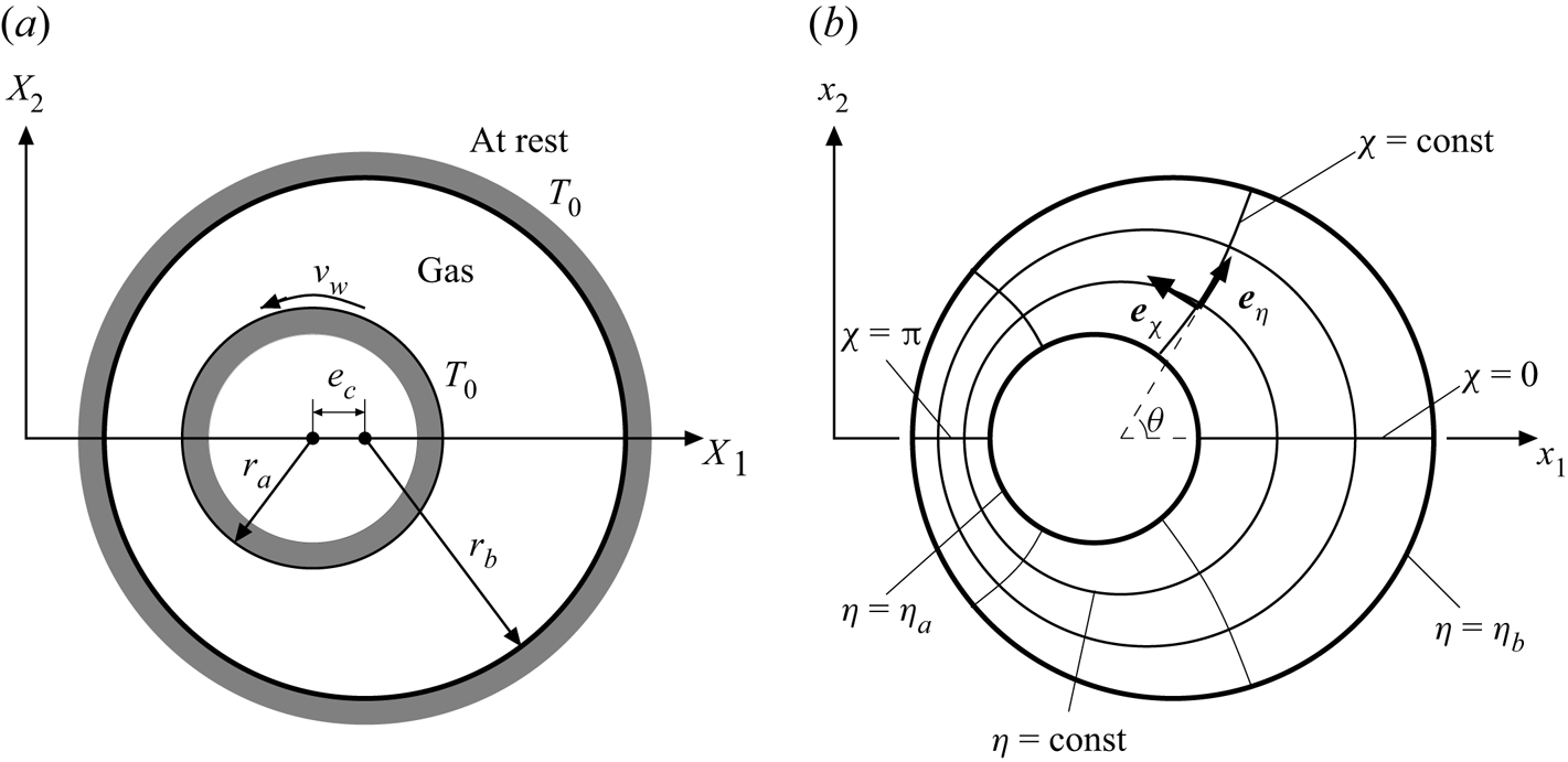
Figure 1. Schematic of the system. (a) Schematic view of the annulus and (b) the bipolar coordinate system ( $\eta, \chi$) in the dimensionless space.
2.2. Basic equation
We introduce the dimensionless variables
 \begin{equation} x_i=\frac{X_i}{r_b-r_a}, \quad \zeta_i=\frac{\xi_i}{(2RT_0)^{1/2}}, \end{equation}
for the spatial rectangular coordinates  $X_i$ and the molecular velocity $\xi _i$. The dimensionless molecular velocity $\zeta _i$ is also denoted by $\boldsymbol {\zeta }$.
In the following analysis, we use the bipolar coordinate system  $\eta, \chi, \zeta _\eta, \zeta _\chi, \zeta _z$, as shown in figure 1(b), defined by
 $$\begin{gather} x_1={-}\frac{a \sinh \eta}{\cosh\eta -\cos\chi}, \quad x_2= \frac{a \sin \chi}{\cosh\eta -\cos\chi}, \end{gather}$$
 $$\begin{gather}\boldsymbol{\zeta}= \zeta_\eta\boldsymbol{e}_\eta +\zeta_\chi\boldsymbol{e}_\chi +\zeta_z\boldsymbol{e}_z, \end{gather}$$
where
 \begin{equation} a= (c\varepsilon)^{{-}1}\left[(1-\varepsilon^2) \left(1+c+\frac{1-\varepsilon^2}{4}c^2\right)\right]^{1/2}. \end{equation}
The scale factor  $h$ defined by $h=[(\partial x_1/\partial \eta )^2 +(\partial x_2/\partial \eta )^2]^{1/2} =[(\partial x_1/\partial \chi )^2 +(\partial x_2/\partial \chi )^2]^{1/2}$ is given by
 \begin{equation} h=\frac{a}{\cosh\eta -\cos\chi}. \end{equation}
The values of  $\eta$ and $\chi$ are in the ranges $\eta _a\le \eta \le \eta _b,\ 0\le \chi < 2{\rm \pi}$, where $\eta _a$ and $\eta _b$ are negative constants
 \begin{equation} \eta_a={-}\text{arcsinh} ca,\quad \eta_b={-}\text{arcsinh} \frac{ca}{1+c},\quad \eta_a<\eta_b<0. \end{equation}
The vectors  $\boldsymbol {e}_\eta$ and $\boldsymbol {e}_\chi$ are unit vectors in the $x_1-x_2$ plane normal to the curves $\eta =\text {const}$ and $\chi =\text {const}$, respectively, and $\boldsymbol {e}_z=\boldsymbol {e}_\eta \times \boldsymbol {e}_\chi$. Note that $ca=\varepsilon ^{-1}(1-\varepsilon ^2)^{1/2}+O(c)$ from (2.5). The dimensionless variable $\hat {f}$ for the velocity distribution function $f$ is defined by
 \begin{equation} \,\hat{f}= \frac{f}{\rho_0(2RT_0)^{{-}3/2}}. \end{equation}
 The dimensionless Boltzmann equation that governs  $\hat {f}(\eta, \chi, \zeta _\eta, \zeta _\chi, \zeta _z)$ in the time-independent state for the axially uniform case is written as (Kogan Reference Kogan1969)
 \begin{equation} \frac{\zeta_\eta}{h}\frac{\partial\hat{f}}{\partial \eta}+\frac{\zeta_\chi}{h}\frac{\partial\hat{f}}{\partial \chi} +\frac{1}{h^2}\left( \zeta_\chi\frac{\partial h}{\partial \eta} -\zeta_\eta\frac{\partial h}{\partial \chi} \right) \left(\zeta_\chi\frac{\partial\hat{f}}{\partial \zeta_\eta} -\zeta_\eta\frac{\partial\hat{f}}{\partial \zeta_\chi}\right)= \frac{1}{k} \hat{J}(\,\hat{f},\hat{f}). \end{equation}
The  $\hat {J}({\cdot },{\cdot })$ is the dimensionless collision integral defined by
 \begin{align} \left.\begin{gathered} \hat{J}(\,\hat{f},\hat{g})= \frac{1}{2}\iint \left[ \hat{f}(\boldsymbol{\zeta}^\prime_*) \hat{g}(\boldsymbol{\zeta}^\prime) +\hat{f}(\boldsymbol{\zeta}^\prime)\hat{g}(\boldsymbol{\zeta}^\prime_*) -\hat{f}(\boldsymbol{\zeta}_*) \hat{g}(\boldsymbol{\zeta}) -\hat{f}(\boldsymbol{\zeta})\hat{g}(\boldsymbol{\zeta}_*)\right] \hat{B} \,\text{d} \varOmega(\boldsymbol{e})\,\mathbf{d}\boldsymbol{\zeta}_*, \\ \boldsymbol{\zeta}^\prime= \boldsymbol{\zeta} +[\boldsymbol{e}\boldsymbol{\cdot}(\boldsymbol{\zeta}_*-\boldsymbol{\zeta})]\boldsymbol{e},\quad \boldsymbol{\zeta}^\prime_*= \boldsymbol{\zeta}_* -[\boldsymbol{e}\boldsymbol{\cdot}(\boldsymbol{\zeta}_*-\boldsymbol{\zeta})]\boldsymbol{e}, \end{gathered}\right\} \end{align}
where  $\boldsymbol {e}$ is a unit vector, $\textrm {d}{\varOmega }(\boldsymbol {e})$ is the solid-angle element in the direction of $\boldsymbol {e}$ and $\mathbf{d}\boldsymbol {\zeta }_*=\textrm {d}\zeta _{\chi *}\, \textrm {d}\zeta _{\eta *}\, \textrm {d}\zeta _{z*}$. The factor $\hat {B}$ is a function of $|\boldsymbol {e}\boldsymbol {\cdot }(\boldsymbol {\zeta }_*-\boldsymbol {\zeta })|/|\boldsymbol {\zeta }_*-\boldsymbol {\zeta }|$ and $|\boldsymbol {\zeta }_*-\boldsymbol {\zeta }|$, and its functional form is determined by the molecular model. In (2.10), the arguments of the spatial variables $\eta$ and $\chi$ are common and are omitted for simplicity. The integration in (2.10) is carried out over the whole direction of $\boldsymbol {e}$ and the whole space of $\boldsymbol {\zeta }$. The range of integration with respect to $\boldsymbol {\zeta }$ is its whole space unless otherwise stated.
The diffuse-reflection boundary condition on the rotating inner cylinder is given by
 \begin{equation} \left.\begin{gathered} \,\hat{f} = {\rm \pi}^{{-}3/2}\hat{\sigma}_{a} \exp(-\zeta_\eta^2 -(\zeta_\chi-\hat{v}_w)^2 -\zeta_z^2),\quad \zeta_\eta>0,\enspace \eta=\eta_a, \\ \hat{\sigma}_{a}={-}2\sqrt{\rm \pi} \int_{\zeta_\eta<0} \zeta_\eta \hat{f} \,\mathbf{d}\boldsymbol{\zeta},\quad \eta=\eta_a. \end{gathered}\right\} \end{equation}
The boundary condition on the outer cylinder at rest is given by
 \begin{equation} \left.\begin{gathered} \,\hat{f} =\hat{\sigma}_{b} E, \quad \zeta_\eta <0,\enspace \eta=\eta_b, \\ \hat{\sigma}_{b}= 2\sqrt{\rm \pi} \int_{\zeta_\eta>0} \zeta_\eta \hat{f} \,\mathbf{d}\boldsymbol{\zeta},\quad \eta=\eta_b, \end{gathered}\right\} \end{equation}
where  $E={\rm \pi} ^{-3/2} \exp (-\boldsymbol {\zeta }^2)$. The periodic condition with respect to $\chi$ is given by
 $$\begin{gather} \hat{f}(\eta, 0, \zeta_\eta, \zeta_\chi, \zeta_z) = \hat{f}(\eta, 2{\rm \pi}, \zeta_\eta, \zeta_\chi, \zeta_z),\quad \zeta_\chi>0, \end{gather}$$
 $$\begin{gather}\hat{f}(\eta, 2{\rm \pi}, \zeta_\eta, \zeta_\chi, \zeta_z) = \hat{f}(\eta, 0, \zeta_\eta, \zeta_\chi, \zeta_z),\quad \zeta_\chi<0. \end{gather}$$
Finally, the average gas density  $\rho _0$ is defined by $\int \!\!\!\int \textrm {d} X_1\, \textrm {d} X_2 \int \! f \,\mathbf{d}\boldsymbol {\xi } = {\rm \pi}(r_b^2-r_a^2)\rho _0$, where the spatial integration is conducted over the annulus region in figure 1(a). In terms of the dimensionless quantities, this equation yields
 \begin{equation} \int_{0}^{2{\rm \pi}} \text{d}\chi \int_{\eta_a}^{\eta_b} \text{d}\eta\, h^2 \int \hat{f} \,\mathbf{d}\boldsymbol{\zeta} = \frac{2{\rm \pi}}{c} \left( 1 +\frac{c}{2} \right). \end{equation}
 The macroscopic variables of the gas, i.e. the density  $\rho$, the flow velocity $v_i$
$v_i$  $(i=\eta, \chi )$, the temperature $T$, the pressure $p$ and the stress tensor $p_{ij}$ $(i=\eta, \chi ; j=\eta, \chi )$ are defined by the moments of the velocity distribution function $f$. The dimensionless variables $\hat {\rho }=\rho /\rho _0$, $\hat {v}_i=v_i/(2RT_0)^{1/2}$, $\hat {T}=T/T_0$, $\hat {p}=p/p_0$ ( $p_0=R\rho _0 T_0$) and $\hat {p}_{ij}=p_{ij}/p_0$ are given by the moments of the dimensionless distribution function $\hat {f}$ as
 $$\begin{gather} \hat{\rho} = \int \hat{f} \,\mathbf{d}\boldsymbol{\zeta}, \end{gather}$$
 $$\begin{gather}\hat{v}_i = \frac{1}{\hat{\rho}} \int \zeta_i \kern0.06em\hat{f} \,\mathbf{d}\boldsymbol{\zeta}, \quad i=\chi, \eta, \end{gather}$$
 $$\begin{gather}\hat{T} = \dfrac{2}{3\hat{\rho}} \int \left[ (\zeta_\eta-\hat{v}_\eta)^2 +(\zeta_\chi-\hat{v}_\chi)^2 +\zeta_z^2\right] \hat{f} \,\mathbf{d}\boldsymbol{\zeta}, \end{gather}$$
 $$\begin{gather}\hat{p}= \hat{\rho} \hat{T}, \end{gather}$$
 $$\begin{gather}\hat{p}_{ij}= 2\int (\zeta_i-\hat{v}_i)(\zeta_j-\hat{v}_j) \hat{f} \,\mathbf{d}\boldsymbol{\zeta}, \quad i=\eta, \chi;\enspace j=\eta, \chi. \end{gather}$$
 Integrating the Boltzmann equation (2.9) over the whole space of  $\zeta _\eta, \zeta _\chi$ and $\zeta _z$, we obtain the equation of continuity
 \begin{equation} \frac{\partial h \hat{\rho} \hat{v}_\eta}{\partial \eta} +\frac{\partial h \hat{\rho} \hat{v}_\chi}{\partial \chi}=0. \end{equation}
 The rectangular components  $(F_1, F_2)$ of the force and the torque $N$ acting on the inner cylinder per unit depth is given by
 $$\begin{gather} \frac{1}{p_0 r_a} \begin{pmatrix} F_1 \\ F_2 \end{pmatrix}={-}\int_{0}^{2{\rm \pi}} \begin{pmatrix} \hat{p}_{\eta\eta} \cos\theta -\hat{p}_{\chi\eta} \sin\theta\\ \hat{p}_{\eta\eta} \sin\theta +\hat{p}_{\chi\eta} \cos\theta \end{pmatrix} ch \,\text{d}\chi,\quad \eta=\eta_a, \end{gather}$$
 $$\begin{gather}\frac{N}{p_0 r_a^2} = \int_{0}^{2{\rm \pi}} \hat{p}_{\chi\eta} ch\, \text{d}\chi,\quad \eta=\eta_a, \end{gather}$$
where  $\theta$ is the angle shown in figure 1(b) defined by
 \begin{equation} \cos\theta= \frac{ \cosh\eta \cos\chi-1}{\cosh\eta -\cos\chi},\quad \sin\theta= \frac{-\sinh\eta \sin\chi }{\cosh\eta -\cos\chi}. \end{equation}
The boundary-value problem given by (2.9)–(2.15) is characterized by the following four dimensionless parameters:
 \begin{equation} c=\frac{r_b-r_a}{r_a}, \quad \varepsilon=\frac{e_c}{r_b-r_a}, \quad \hat{v}_w=cu_w=\frac{v_w}{(2RT_0)^{1/2}},\quad k=\frac{\sqrt{\rm \pi}}{2} \frac{\ell}{r_b-r_a}. \end{equation}
We study this problem under the condition (2.1a–c).
2.3. Some transformations
For convenience of the analysis, we introduce the change of independent variables from  $\eta, \zeta _\eta$ and $\zeta _\chi$ to $y, \zeta _\rho$ and $\theta _\zeta$ as follows (Sugimoto & Sone Reference Sugimoto and Sone1992):
 \begin{equation} \eta= \eta_a +(\eta_b-\eta_a)y, \quad \zeta_\eta=\zeta_\rho\cos\theta_\zeta, \quad \zeta_\chi=\zeta_\rho\sin\theta_\zeta,\end{equation}
where  $0\le y\le 1,\ 0\le \zeta _\rho <\infty$ and $-{\rm \pi} <\theta _\zeta \le {\rm \pi}$. In terms of the new variables $y, \zeta _\rho, \theta _\zeta$ and $\chi$, the boundary-value problem (2.9)–(2.15) is rewritten as follows. The Boltzmann equation is
 \begin{equation} \frac{\zeta_\rho\cos\theta_\zeta}{\gamma H} \frac{\partial\hat{f}}{\partial y} +c\frac{\zeta_\rho\sin\theta_\zeta}{H} \frac{\partial\hat{f}}{\partial \chi} -c\zeta_\rho G \frac{\partial\hat{f}}{\partial \theta_\zeta}= \frac{1}{k} \hat{J}(\,\hat{f},\hat{f}), \end{equation}
where
 \begin{align} H=ch=\frac{-\sinh\eta_a}{\cosh\eta -\cos\chi}, \quad G=\frac{-\sinh\eta \sin\theta_\zeta +\sin\chi \cos\theta_\zeta}{-\sinh\eta_a}, \quad \gamma=\frac{\eta_b-\eta_a}{c}. \end{align}
In (2.24a–c) and in what follows,  $\eta$ should be understood as $\eta (y)$ by (2.22a). Note that $H, G$ and $\gamma$ are of $O(1)$. The boundary conditions (2.11)–(2.14) and the subsidiary condition (2.15) are transformed into
 $$\begin{gather} \,\hat{f} = {\rm \pi}^{{-}3/2}\hat{\sigma}_{a} \exp( -\zeta_\rho^2 +2c u_w\zeta_\rho\sin\theta_\zeta -c^2 u_w^2 -\zeta_z^2),\quad \cos\theta_\zeta>0,\enspace y=0, \end{gather}$$
 $$\begin{gather}\,\hat{f} =\hat{\sigma}_{b} E, \quad \cos\theta_\zeta<0,\enspace y=1, \end{gather}$$
 \begin{gather} \left.\begin{gathered} \hat{\sigma}_{a}={-}2\sqrt{\rm \pi} \int\!\!\! \int\!\!\! \int_{\cos\theta_\zeta<0} \zeta_\rho^2\cos\theta_\zeta \kern0.06em\hat{f}\, \text{d}\zeta_\rho\, \text{d}\theta_\zeta\, \text{d}\zeta_z, \quad y=0, \\ \hat{\sigma}_{b}= 2\sqrt{\rm \pi} \int\!\!\! \int\!\!\! \int_{\cos\theta_\zeta>0} \zeta_\rho^2\cos\theta_\zeta \kern0.06em\hat{f}\, \text{d}\zeta_\rho\, \text{d}\theta_\zeta\, \text{d}\zeta_z, \quad y=1, \end{gathered}\right\} \end{gather}
 $$\begin{gather} \hat{f}(y, 0, \zeta_\rho, \theta_\zeta, \zeta_z)= \hat{f}(y, 2{\rm \pi}, \zeta_\rho, \theta_\zeta, \zeta_z),\quad \theta_\zeta>0, \end{gather}$$
 $$\begin{gather}\hat{f}(y, 2{\rm \pi}, \zeta_\rho, \theta_\zeta, \zeta_z) = \hat{f}(y, 0, \zeta_\rho, \theta_\zeta, \zeta_z),\quad \theta_\zeta<0, \end{gather}$$
 $$\begin{gather}\int_{0}^{2{\rm \pi}} \text{d}\chi \int_{0}^{1} \text{d} y\, H^2 \int\!\!\! \int \!\!\! \int \zeta_\rho \,\hat{f}\, \text{d}\zeta_\rho\, \text{d}\theta_\zeta\, \text{d}\zeta_z = \frac{2{\rm \pi}}{\gamma}\left(1+\frac{c}{2}\right), \end{gather}$$
where  $E={\rm \pi} ^{-3/2}\exp (-\zeta _\rho ^2-\zeta _z^2)$ in the new variables. Here, and in what follows, we use the convention that $\hat {f}(\eta (y), \chi, \zeta _\eta (\zeta _\rho, \theta _\zeta ), \zeta _\chi (\zeta _\rho, \theta _\zeta ), \zeta _z)$ is simply written as $\hat {f}(y, \chi, \zeta _\rho, \theta _\zeta, \zeta _z)$ because no confusion will arise. The ranges of integration with respect to $\zeta _\rho, \theta _\zeta$ and $\zeta _z$ are, respectively, $0<\zeta _\rho <\infty$, $-{\rm \pi} <\theta _\zeta <{\rm \pi}$ and $-\infty <\zeta _z<\infty$ unless otherwise stated.
The macroscopic variables are
 $$\begin{gather} \hat{\rho} = \int \!\!\! \int \!\!\! \int \zeta_\rho \,\hat{f}\, \text{d}\zeta_\rho\, \text{d}\theta_\zeta\, \text{d}\zeta_z, \end{gather}$$
 $$\begin{gather}\hat{v}_\eta = \dfrac{1}{\hat{\rho}} \int \!\!\! \int \!\!\! \int \zeta_\rho^2\cos\theta_\zeta \,\hat{f}\, \text{d}\zeta_\rho\, \text{d}\theta_\zeta\, \text{d}\zeta_z, \end{gather}$$
 $$\begin{gather}\hat{v}_\chi = \dfrac{1}{\hat{\rho}} \int \!\!\! \int \!\!\! \int \zeta_\rho^2\sin\theta_\zeta \,\hat{f}\, \text{d}\zeta_\rho\, \text{d}\theta_\zeta\, \text{d}\zeta_z, \end{gather}$$
 $$\begin{gather}\hat{T} = \dfrac{2}{3\hat{\rho}} \int \!\!\! \int \!\!\! \int \zeta_\rho \left[ (\zeta_\rho\cos\theta_\zeta-\hat{v}_\eta)^2 +(\zeta_\rho\sin\theta_\zeta-\hat{v}_\chi)^2 +\zeta_z^2 \right] \hat{f}\, \text{d}\zeta_\rho\, \text{d}\theta_\zeta\, \text{d}\zeta_z, \end{gather}$$
 $$\begin{gather}\hat{p}= \hat{\rho} \hat{T}, \end{gather}$$
 $$\begin{gather}\hat{p}_{\eta\eta}= 2\int \!\!\! \int \!\!\! \int \zeta_\rho(\zeta_\rho\cos\theta_\zeta-\hat{v}_\eta)^2 \,\hat{f}\, \text{d}\zeta_\rho\, \text{d}\theta_\zeta\, \text{d}\zeta_z, \end{gather}$$
 $$\begin{gather}\hat{p}_{\chi\eta}= \hat{p}_{\eta\chi}= 2\int \!\!\! \int \!\!\! \int \zeta_\rho(\zeta_\rho\cos\theta_\zeta-\hat{v}_\eta)(\zeta_\rho\sin\theta_\zeta-\hat{v}_\chi) \,\hat{f}\, \text{d}\zeta_\rho\, \text{d}\theta_\zeta\, \text{d}\zeta_z. \end{gather}$$
 Changing the variable  $\eta$ into $y$ using (2.22a), integrating (2.17) with respect to $y$ from 0 to 1 and applying the boundary condition (2.25) or (2.26), we obtain the mass conservation law
 \begin{equation} \frac{\text{d}}{\text{d} \chi}\int_0^1 H \hat{\rho} \hat{v}_\chi\,\text{d} y = 0. \end{equation}
3. Analysis
3.1. Preliminary remarks and plan of analysis
We seek a solution of the boundary-value problem (2.23)–(2.30) for small  $c$. Note that the second and the third terms on the left-hand side of (2.23) are multiplied by $c$. The third term $-c\zeta _\rho G \partial \hat {f}/\partial \theta _\zeta$, which is peculiar to a curvilinear coordinate system, will be called the curvature term for short. Then, one may consider it feasible to seek a solution using a perturbation by regarding these two terms as higher-order terms. We seek the solution as a power series expansion in $c$
$c$
 \begin{equation} \,\hat{f}= \,\hat{f}_{(0)} +\,\hat{f}_{(1)}c + \cdots. \end{equation}
Substituting (3.1) into the boundary-value problem reduces it to a sequence of boundary-value problems of the Boltzmann equation with only one derivative term with  $\partial \hat {f}_{(m)}/\partial y \ (m=0, 1, \ldots )$; other derivative terms with $\partial \hat {f}_{(m)}/\partial \chi$ and $\partial \hat {f}_{(m)}/\partial \theta _\zeta$ will appear as inhomogeneous terms. However, this perturbation analysis results in a lubrication equation that fails to approximate the solution of the Boltzmann equation for large Knudsen numbers. The reason is as follows (Doi Reference Doi2022).
Suppose that the dimensionless curvature  $c$ is small but the Knudsen number $k$ is so large that $ck^2=O(1)$. The velocity distribution function will then consist of that of the molecules arriving from the two cylinders without collisions. Figure 2(a) shows a schematic of molecular trajectories arriving at a point from the inner and the outer cylinders. The shaded area represents the range of direction of the molecular velocities arriving from the rotating inner cylinder. It is clear from figure 2(a) that this range from the inner cylinder is smaller than that from the outer cylinder at rest. In figure 2(b), this difference in the angle is denoted by $2\varphi$. From figure 2(b), we see that $\cos \varphi =c^{-1}/(c^{-1}+y)$, and this yields $\varphi \simeq (2yc)^{1/2}$ because $c$ and thus $\varphi$ are small. Thus, the gas behaviour is affected by the curvature by $O(c^{1/2})$ which is much larger than $c$. On the other hand, if we regard the curvature term of (2.23) as a higher-order term, then the characteristics of (2.23) and thus the molecular trajectories are no longer straight, and the angle of the shaded area becomes ${\rm \pi}$ (Doi Reference Doi2022); so the range of direction of the molecular velocities from the rotating inner cylinder is overestimated by an amount proportional to $c^{1/2}$. Thus, simply treating the curvature term as a higher-order term produces a non-negligible error of $O(c^{1/2})$. For example, the macroscopic flow velocity will be estimated to be greater than its actual value. Clearly, this is a non-continuum effect arising from the finite nature of the mean free path. This fact was pointed out in Doi (Reference Doi2022) for a lubrication flow between coaxial cylinders, and an error of $O(c^{1/2})$ was numerically demonstrated. A more detailed discussion is given in Doi (Reference Doi2022). It is quite possible that a similar phenomenon also occurs in the present case of an eccentric annulus.

Figure 2. Characteristics or trajectories of collisionless molecules. (a) Characteristics of the true Boltzmann equation (2.23), where the shaded area represents the range of direction of molecular velocities arriving from the inner cylinder. (b) Schematic showing that the angle of the shaded area in (a) is smaller than  ${\rm \pi}$ by $O(c^{1/2})$, specifically, $\varphi \simeq (2yc)^{1/2}$. Note that the dimensionless radius of the inner cylinder is $1/c$.
The above discussion suggests that the key to the correct analysis lies in describing the characteristics of the Boltzmann equation (2.23) correctly. To this end, it is suggested in Doi (Reference Doi2022) that the curvature term should not be treated as a higher-order term but dealt with the first term of (2.23) as a whole, regardless of the magnitude of  $c$. Specifically, let us define the operator
 \begin{equation} \mathcal{D}_{ec}= \frac{\cos\theta_\zeta}{\gamma H}\frac{\partial}{\partial y} -cG\frac{\partial}{\partial \theta_\zeta}. \end{equation}
In terms of  $\mathcal {D}_{ec}$, the Boltzmann equation is written as
 \begin{equation} \zeta_\rho\mathcal{D}_{ec}\,\hat{f} +c\frac{\zeta_\rho\sin\theta_\zeta}{H}\frac{\partial\hat{f}}{\partial \chi} = \frac{1}{k}\hat{J}(\,\hat{f},\hat{f}). \end{equation}
The solution is sought in the power series expansion (3.1). Here,  $\mathcal {D}_{ec}$ is not expanded in $c$ but treated as a whole. Namely, we assume
 \begin{equation} \mathcal{D}_{ec}\,\hat{f} = \mathcal{D}_{ec}\,\hat{f}_{(0)}+\mathcal{D}_{ec}\,\hat{f}_{(1)} c +\cdots,\quad \mathcal{D}_{ec}\,\hat{f}_{(m)}\sim \,\hat{f}_{(m)}\quad (m=0, 1, \ldots). \end{equation}
To be precise, the assumption (3.4b) is inconsistent in the range  $|\theta _\zeta -{\rm \pi} /2|=O(c)$. However, it is expected that this discrepancy is localized within a so narrow range in the molecular velocity space that an influence on the macroscopic variable is small (Doi Reference Doi2022). Using this approach, the projection of the characteristics of the Boltzmann equation on the $\theta _\zeta -y$ plane at each stage of approximation is maintained. Substituting (3.1) and (3.4a) into (3.3) and (2.25)–(2.30) and formally arranging the terms of the same order in $c$, we obtain a sequence of boundary-value problems that determine $\hat {f}_{(0)}, \hat {f}_{(1)}, \ldots$ successively from the lowest order as described in the next subsection.
3.2. Leading- and first-order solutions
The boundary-value problem that governs the leading-order solution  $\hat {f}_{(0)}$ is given by
 $$\begin{gather} \zeta_\rho\mathcal{D}_{ec}\kern0.06em\hat{f}_{(0)} = \frac{1}{k} \hat{J}(\,\hat{f}_{(0)}, \,\hat{f}_{(0)}), \end{gather}$$
 $$\begin{gather}\,\hat{f}_{(0)} = \hat{\sigma}_{a(0)} E, \quad \cos\theta_\zeta>0,\enspace y=0, \end{gather}$$
 $$\begin{gather}\,\hat{f}_{(0)} = \hat{\sigma}_{b(0)} E, \quad \cos\theta_\zeta<0,\enspace y=1, \end{gather}$$
 \begin{gather} \left.\begin{gathered} \hat{\sigma}_{a(0)}={-}2\sqrt{\rm \pi} \iint\!\!\!\int_{\cos\theta_\zeta<0} \zeta_\rho^2\cos\theta_\zeta \kern0.06em\hat{f}_{(0)}\, \text{d}\zeta_\rho\, \text{d}\theta_\zeta\, \text{d}\zeta_z,\quad y=0, \\ \hat{\sigma}_{b(0)}= 2\sqrt{\rm \pi} \iint\!\!\!\int_{\cos\theta_\zeta>0} \zeta_\rho^2\cos\theta_\zeta \kern0.06em\hat{f}_{(0)}\, \text{d}\zeta_\rho\, \text{d}\theta_\zeta\, \text{d}\zeta_z, \quad y=1, \end{gathered}\right\} \end{gather}
 \begin{gather} \int_0^{2{\rm \pi}} \text{d}\chi \int_{0}^{1}\text{d} y\, H^2 \iint\!\!\! \int \zeta_\rho \kern0.06em\hat{f}_{(0)} \,\text{d}\zeta_\rho \,\text{d}\theta_\zeta \,\text{d}\zeta_z = \frac{2{\rm \pi}}{\gamma}. \end{gather}
Equations (3.5)–(3.7) can be solved independently at each  $\chi$ because the derivative term $\partial \hat {f}_{(0)}/\partial \chi$ is absent. A solution is an equilibrium state at rest
 \begin{equation} \,\hat{f}_{(0)} = C_{(0)} E, \end{equation}
where  $C_{(0)}$ may be an arbitrary function of $\chi$ as long as (3.8) is satisfied. The factor $C_{(0)}$ can be related to a macroscopic variable. Substituting the expansion (3.1) into (2.31a)–(2.31e), the macroscopic variables can be expanded in $c$, e.g. $\hat {\rho } = \hat {\rho }_{(0)} + \hat {\rho }_{(1)} c + \cdots$. At the leading order, we obtain from (3.10) that
 \begin{equation} \hat{\rho}_{(0)} = C_{(0)}, \quad \hat{v}_{\eta(0)} = \hat{v}_{\chi(0)} = 0, \quad \hat{T}_{(0)}=1, \quad \hat{p}_{(0)}= C_{(0)}. \end{equation}
Thus,  $C_{(0)}$ is identified with the leading-order pressure $\hat {p}_{(0)}$. We henceforth write $\hat {p}_{(0)}$ for $C_{(0)}$. Incidentally, we obtain $\hat {\sigma }_{a(0)}=\hat {\sigma }_{b(0)}=\hat {p}_{(0)}$ and $\int \!\!\!\int \!\!\! \int \zeta _\rho \hat {f}_{(0)} \,\textrm {d}\zeta _\rho \,\textrm {d}\theta _\zeta \,\textrm {d}\zeta _z=\hat {\rho }_{(0)}=\hat {p}_{(0)}$.
The boundary-value problem for the first-order solution  $\hat {f}_{(1)}$ is a linear and inhomogeneous one given by
 $$\begin{gather} \zeta_\rho\mathcal{D}_{ec}\kern0.06em\hat{f}_{(1)} = \frac{2}{k} \hat{J}(\,\hat{f}_{(0)}, \,\hat{f}_{(1)}) -\frac{\zeta_\rho\sin\theta_\zeta}{H} \frac{\partial \,\hat{f}_{(0)}}{\partial \chi}, \end{gather}$$
 $$\begin{gather}\,\hat{f}_{(1)} = \left( \hat{\sigma}_{a(1)} + 2 u_w\hat{p}_{(0)} \zeta_\rho\sin\theta_\zeta \right) E, \quad \cos\theta_\zeta>0,\enspace y=0, \end{gather}$$
 $$\begin{gather}\,\hat{f}_{(1)} = \hat{\sigma}_{b(1)} E, \quad \cos\theta_\zeta<0,\enspace y=1, \end{gather}$$
 \begin{gather} \left.\begin{gathered} \hat{\sigma}_{a(1)}={-}2\sqrt{\rm \pi} \iint\!\!\!\int_{\cos\theta_\zeta<0} \zeta_\rho^2\cos\theta_\zeta \kern0.06em\hat{f}_{(1)} \,\text{d}\zeta_\rho \,\text{d}\theta_\zeta \,\text{d}\zeta_z, \quad y=0, \\ \hat{\sigma}_{b(1)}= 2\sqrt{\rm \pi} \iint\!\!\!\int_{\cos\theta_\zeta>0} \zeta_\rho^2\cos\theta_\zeta \kern0.06em\hat{f}_{(1)} \,\text{d}\zeta_\rho \,\text{d}\theta_\zeta \,\text{d}\zeta_z, \quad y=1, \end{gathered}\right\} \end{gather}
 \begin{gather} \int_0^{2{\rm \pi}}\text{d}\chi \int_{0}^{1}\text{d} y\, H^2\int\!\!\! \int\!\!\! \int \zeta_\rho \kern0.06em\hat{f}_{(1)} \,\text{d}\zeta_\rho \,\text{d}\theta_\zeta \,\text{d}\zeta_z = \frac{\rm \pi}{\gamma}.\end{gather}
To analyse this, we introduce an approximation: the operator  $\mathcal {D}_{ec}$ in (3.12) is simplified to
 \begin{equation} \mathcal{D}_{ec}'= \frac{\cos\theta_\zeta}{\gamma H}\frac{\partial}{\partial y} -c\frac{\sinh\eta \sin\theta_\zeta}{\sinh\eta_a} \frac{\partial}{\partial \theta_\zeta}, \end{equation}
omitting the term  $\sin \chi \cos \theta _\zeta$ in $G$. This approximation may be permissible because the curvature term is crucial for the molecular velocities nearly tangential to the inner cylinder, i.e. around $\theta _\zeta =\pm {\rm \pi}/2$ (see figure 2a), at which the omitted term $\sin \chi \cos \theta _\zeta$ vanishes. As we will see in § 5, this approximation is sufficient for the purpose of this paper. Owing to this approximation, the operator $\mathcal {D}_{ec}^\prime$ preserves the parity with respect to $\theta _\zeta$. As a result, we can decompose the solution $\hat {f}_{(1)}$ into a sum of even and odd functions with respect to $\theta _\zeta$ as $\hat {f}_{(1)}=\hat {f}_{(1)}^{even}+\hat {f}_{(1)}^{odd}$. The even function $\hat {f}_{(1)}^{even}$ is a solution of the homogeneous Boltzmann equation that is responsible for $\hat {\sigma }_{a(1)}, \hat {\sigma }_{b(1)}$ and the subsidiary condition (3.16). A solution is a Maxwellian at rest
 \begin{equation} \,\hat{f}_{(1)}^{even} = C_{(1)} E, \end{equation}
where  $C_{(1)}$ is an arbitrary function of $\chi$ subject to (3.16). The odd function $\hat {f}_{(1)}^{odd}$ is the particular solution that is responsible for the inhomogeneous terms. By putting $\hat {f}_{(1)}^{odd}=\hat {f}_{(0)} \phi$, the problem for $\hat {f}_{(1)}^{odd}$ can be reduced to a simpler problem for $\phi$
 $$\begin{gather} \zeta_\rho\mathcal{D}_{ec}' \phi = \frac{\hat{p}_{(0)}}{k} \mathcal{L}(\phi) -\frac{\zeta_\rho\sin\theta_\zeta}{H} \frac{1}{\hat{p}_{(0)}} \frac{\text{d} \hat{p}_{(0)}}{\text{d} \chi}, \end{gather}$$
 $$\begin{gather}\phi = 2 u_w \zeta_\rho\sin\theta_\zeta, \quad \cos\theta_\zeta>0,\enspace y=0, \end{gather}$$
 $$\begin{gather}\phi = 0, \quad \cos\theta_\zeta<0,\enspace y=1, \end{gather}$$
where  $\mathcal {L}({\cdot })$ is the linearized collision operator defined by $E\mathcal {L}(\phi )=2\hat {J}(E,E\phi )$. Because of the linearity, the solution is given by
 \begin{equation} \phi(y, \chi, \boldsymbol{\zeta}) = \frac{1}{\hat{p}_{(0)}} \frac{\text{d} \hat{p}_{(0)}}{\text{d} \chi} \varPhi_{Pec}\left(y, \boldsymbol{\zeta}; \frac{k}{\hat{p}_{(0)}}, \chi \right) +u_w \varPhi_{Cec}\left(y, \boldsymbol{\zeta}; \frac{k}{\hat{p}_{(0)}}, \chi \right), \end{equation}
where  $\boldsymbol {\zeta }$ is an abbreviation for $(\zeta _\rho, \theta _\zeta, \zeta _z)$. The functions $\varPhi _{Pec}(y, \boldsymbol {\zeta }; \tilde {k}, \chi )$ and $\varPhi _{Cec}(y, \boldsymbol {\zeta }; \tilde {k}, \chi )$ are defined by (A1) and (A2) and (A3)–(A5), respectively, in Appendix A; they depend on $c$ and $\varepsilon$ through the operator $\mathcal {D}_{ec}^\prime$. The parameter $\tilde {k}$ stands for $k/\hat {p}_{(0)}$, which may be termed a local Knudsen number due to the variation of the pressure $\hat {p}_{(0)}$.
Substituting (3.10), (3.18) and (3.22) into (3.1), the solution up to  $\hat {f}=\hat {f}_{(0)} +\hat {f}_{(1)} c$ is written as
 \begin{align} & \hat{f}(y, \chi, \boldsymbol{\zeta}) = \hat{p}_{(0)} E \nonumber\\ &\quad \times \left\{1 +c\left[\frac{C_{(1)}}{\hat{p}_{(0)}} +\frac{1}{\hat{p}_{(0)}} \frac{\text{d} \hat{p}_{(0)}}{\text{d} \chi} \varPhi_{Pec}\left(y, \boldsymbol{\zeta}; \frac{k}{\hat{p}_{(0)}}, \chi \right) +u_w \varPhi_{Cec}\left(y, \boldsymbol{\zeta}; \frac{k}{\hat{p}_{(0)}}, \chi \right)\right]\right\}, \end{align}
in terms of the undetermined functions  $\hat {p}_{(0)}$ and $C_{(1)}$.
It may be noted that there are more several advantages of the approximation (3.17). In addition to the solution  $\phi$ being odd in $\theta _\zeta$, it is also symmetric with respect to $\chi ={\rm \pi}$. Further, the characteristic equation $\gamma H\textrm {d} y/\cos \theta _\zeta = -\sinh \eta _a \textrm {d}\theta _\zeta /(c\sinh \eta \sin \theta _\zeta )$ of (3.19), or written explicitly in the original variables $\eta$ as
 \begin{equation} \frac{\text{d}\eta}{(\cosh\eta-\cos\chi)\cos\theta_\zeta} =\frac{\text{d}\theta_\zeta}{\sinh\eta \sin\theta_\zeta}, \end{equation}
can be solved analytically to yield
 \begin{equation} \frac{\sin\theta_\zeta}{\cosh\eta-\cos\chi}=\text{const}. \end{equation}
These properties are convenient for an accurate numerical analysis of the boundary-value problems (A1) and (A2) and (A3)–(A5) of the two-dimensional Boltzmann equation to obtain  $\varPhi _{Pec}$ and $\varPhi _{Cec}$.
3.3. Lubrication equation
Our next task is to determine the unknown function  $\hat {p}_{(0)}$, and this is accomplished by using the mass conservation law. Substituting (3.23) into (2.31c) and then into (2.32), we obtain from the first-order mass conservation
 \begin{equation} \frac{\text{d}}{\text{d}\chi}\left[m_{Pec}\left(\frac{k}{\hat{p}_{(0)}}, \chi \right) \frac{\text{d} \hat{p}_{(0)}}{\text{d}\chi} +u_w\hat{p}_{(0)}m_{Cec}\left(\frac{k}{\hat{p}_{(0)}}, \chi \right)\right]=0, \end{equation}
where the functions  $m_{Pec}(\tilde {k}, \chi )$ and $m_{Cec}(\tilde {k}, \chi )$, which depend on $c$ and $\varepsilon$, are defined by (A9) in Appendix A. As we are about to see, (3.26) plays a role of determining the leading-order pressure $\hat {p}_{(0)}$.
Suppose that the boundary-value problem (A1) and (A2) for  $\varPhi _{Pec}$ and that (A3)–(A5) for $\varPhi _{Cec}$ are solved over a wide range of the parameters $\tilde {k}, \chi, c$ and $\varepsilon$, and that the database of the functions $m_{Pec}(\tilde {k}, \chi )$ and $m_{Cec}(\tilde {k}, \chi )$ is known. Then, (3.26), (3.9) and the periodic condition constitute the ordinary differential equation to determine $\hat {p}_{(0)}$. Once $\hat {p}_{(0)}$ is known, the velocity distribution function is given by (3.23). Substituting (3.23) into (2.31a)–(2.31g), the macroscopic variables are obtained. For example, the component $\hat {v}_\chi$ of the flow velocity, those of the stress tensor and the pressure $\hat {p}$ up to the non-trivial leading orders are given by
 $$\begin{gather} \hat{v}_{\chi}= c\left[\frac{1}{\hat{p}_{(0)}} \frac{\text{d} \hat{p}_{(0)}}{\text{d}\chi} u_{Pec}\left(y; \frac{k}{\hat{p}_{(0)}}, \chi \right) +u_w u_{Cec}\left(y; \frac{k}{\hat{p}_{(0)}}, \chi \right)\right], \end{gather}$$
 $$\begin{gather}\hat{p}_{\eta\eta}=\hat{p}=\hat{p}_{(0)}, \end{gather}$$
 $$\begin{gather}\hat{p}_{\chi\eta}= c\left[ \frac{\text{d} \hat{p}_{(0)}}{\text{d}\chi} S_{Pec}\left(y; \frac{k}{\hat{p}_{(0)}}, \chi \right) +u_w\hat{p}_{(0)} S_{Cec}\left(y; \frac{k}{\hat{p}_{(0)}}, \chi \right) \right], \end{gather}$$
where the functions  $u_{Pec}(y; \tilde {k}, \chi )$ and $u_{Cec}(y; \tilde {k}, \chi )$ are defined by (A7), and the functions $S_{Pec}(y; \tilde {k}, \chi )$ and $S_{Cec}(y; \tilde {k}, \chi )$ are defined by (A8). Substituting (3.28) and (3.29) into (2.18) and (2.19), the eccentric force and the torque are obtained. Thus, (3.26) plays the role of determining the pressure distribution $\hat {p}_{(0)}$. In this sense, (3.26) may be called a generalized Reynolds equation.
The function  $C_{(1)}$ is as yet undetermined. So, unlike the coaxial case (Doi Reference Doi2022), the truncation error of the solution at this stage is still $O(c)$. To determine $C_{(1)}$, the next-order analysis is necessary, which is briefly touched on in Appendix B. Instead of conducting the precise analysis, however, it is proposed in Appendix B to solve (3.26) subject to the modified subsidiary condition
 \begin{equation} \int_0^{2{\rm \pi}} \text{d}\chi \int_{0}^{1}\text{d} y\, H^2 \hat{p}_{(0)} = \frac{2{\rm \pi}}{\gamma} \left(1+\frac{c}{2}\right) ,\end{equation}
in place of (3.8). Provided that the nonlinear collision integral  $\hat {J}(\,\hat {f}_{(1)},\hat {f}_{(1)})$ in the second-order analysis is negligibly small, this solution $\hat {p}_{(0)}$ yields $\hat {p}$ and the normal stress $\hat {p}_{\eta \eta }$ approximately up to the first order in $c$. Incidentally, when the Mach number based on the lubrication motion is not small in contrast to (2.1b), the difference between the normal stress and the pressure is non-negligible (Ansumali et al. Reference Ansumali, Karlin, Arcidiacono, Abbas and Prasianakis2007).
In the derivation of (3.26), we implicitly assumed that the Knudsen number  $k$ is of $O(1)$. By a similar analysis to that in Doi (Reference Doi2022), we can show that the Reynolds equation for $k=c^{-n} (n=1, 2, \ldots )$ is given by (3.26) in which the functions $m_{Pec}(\tilde {k}, \chi )$ and $m_{Cec}(\tilde {k}, \chi )$ are replaced by $m_{Pec}(\infty, \chi )$ and $m_{Cec}(\infty, \chi )$, respectively. Thus, we find that (3.26) holds up to $k=\infty$ by making $n\to \infty$. Incidentally, the lubrication model (3.26) reduces to that for a coaxial annulus derived in Doi (Reference Doi2022) in the limit $\varepsilon \to 0$ keeping $c$ constant. Details are given in Appendix C.
3.4. Flow-rate coefficients
Equation (3.26) is similar to the conventional Reynolds equation for a one-dimensional and time-independent state, but there are two differences. First, the coefficients of the mass flow rates of Poiseuille and Couette flows in the latter are replaced by the functions  $m_{Pec}(\tilde {k}, \chi )$ and $m_{Cec}(\tilde {k}, \chi )$. That is, the non-continuum effect is condensed in these functions; it is characterized by the first argument $\tilde {k}=k/\hat {p}_{(0)}$. These are determined by the solutions of flow problems of a rarefied gas as follows. The first function $m_{Pec}$ is determined by the solution $\varPhi _{Pec}$ of a flow induced by a pressure gradient imposed along a curved channel. The second function $m_{Cec}$ is determined by the solution $\varPhi _{Cec}$ of a flow along a curved channel induced by a tangential motion of one of the walls. In this sense, the functions $m_{Pec}$ and $m_{Cec}$ may be called the flow-rate coefficients of generalized Poiseuille and Couette flows. Second, the gas-film thickness is absent; it is incorporated into the functions $m_{Pec}$ and $m_{Cec}$. Because the generalized Poiseuille and Couette flows cannot be solved analytically unlike the Navier–Stokes system, we cannot establish an explicit expression of the coefficients in terms of the gas-film thickness. The variation of the gas-film thickness along the channel is characterized by the second argument $\chi$.
Some examples of the flow-rate coefficients are presented in figure 3 for the BGKW kinetic model. Figures 3(a) and 3(b) show, respectively,  $-m_{Pec}$ and $m_{Cec}$ as functions of $\tilde {k}$ and $\chi$ for $\varepsilon =0.1$ and 0.9 with $c=0.05$. These functions are symmetric with respect to $\chi ={\rm \pi}$, and thus only $0\le \chi \le {\rm \pi}$ is shown. When the eccentricity $\varepsilon$ is vanishingly small, the flow is axially symmetric and these functions are thus independent of the longitudinal coordinate $\chi$. The results for $\varepsilon =0.1$ assume this tendency. The function $-m_{Pec}$ of generalized Poiseuille flow shows a slight Knudsen minimum about $\tilde {k}=1$. As the eccentricity $\varepsilon$ approaches unity, both flow rates shrink around $\chi ={\rm \pi}$ at which the channel is narrowest. A simple database of the functions $m_{Pec}$ and $m_{Cec}$ is given in Appendix D. The numerical data necessary for this database are provided by the author via Doi (Reference Doi2023) for wide ranges of the parameters $c$ and $\varepsilon$.

Figure 3. Flow-rate coefficients  $m_{Pec}$ and $m_{Cec}$ for $\varepsilon =0.1$ and 0.9 ( $c=0.05$) as functions of $\tilde {k}$ and $\chi$ (BGKW model); (a) $-m_{Pec}$ and (b) $m_{Cec}$. Dotted line for $\varepsilon =0.1$ and solid line for $\varepsilon =0.9$. These functions are symmetric with respect to $\chi ={\rm \pi}$.
3.5. Lubrication equation without the curvature term
Let us now look back to § 3.1 and discuss what happens if we conduct the perturbation (3.1) by treating the curvature term of (2.23) as a higher-order term. The analysis is quite similar to that in §§ 3.2 and 3.3, and thus only the final result is presented here, leaving the derivation to Appendix E. The lubrication equation thus obtained is
 \begin{equation} \frac{\text{d}}{\text{d}\chi}\left[m_{Pwoc}\left(\frac{k}{\hat{p}_{(0)}}, \chi\right) \frac{\text{d} \hat{p}_{(0)}}{\text{d}\chi}+u_w\hat{p}_{(0)} m_{Cwoc} \left(\frac{k}{\hat{p}_{(0)}}, \chi \right)\right]=0. \end{equation}
Equation (3.31) is of the same form as (3.26); the only difference is that the functions  $m_{Pec}$ and $m_{Cec}$ are replaced, respectively, by $m_{Pwoc}$ and $m_{Cwoc}$ defined by (E10). For discrimination, let us call (3.31) the lubrication model without the curvature term, or the WOC model for short. In contrast, let us call (3.26) the improved model. One of our major objectives is to demonstrate that the solution of the WOC model produces an error of $O(c^{1/2})$ when the Knudsen number is large.
We have now derived two lubrication models, namely, improved model (3.26) and the WOC model (3.31). Our remaining task is to assess whether the solutions of these models approximate that of the Boltzmann equation. For this assessment, accurate solution of the Boltzmann equation is required as a reference. This solution is provided in § 4. The remainder of this paper is devoted to this assessment.
4. Numerical analysis
4.1. Preliminaries
In this section, a direct numerical analysis of the boundary-value problem (2.23)–(2.30) is conducted. In this numerical analysis, we assume that the gas is governed by the BGKW kinetic equation. That is, the collision integral is given by
 \begin{equation} \left.\begin{gathered} \hat{J}(\,\hat{f}, \,\hat{f})= \hat{\rho}( \,\hat{f}_e -\,\hat{f} ), \\ \,\hat{f}_e= \frac{\hat{\rho}}{({\rm \pi}\hat{T})^{3/2}} \exp \left(-\frac{ (\zeta_\rho\cos\theta_\zeta-\hat{v}_\eta)^2 + (\zeta_\rho\sin\theta_\zeta-\hat{v}_\chi)^2 +\zeta_z^2}{\hat{T}}\right), \end{gathered}\right\} \end{equation}
where  $\hat {\rho }, \hat {v}_\eta, \hat {v}_\chi$ and $\hat {T}$ are given by (2.31a)–(2.31d). The mean free path $\ell$ of the BGKW model is related to the viscosity $\mu$ of the gas by (Sone Reference Sone2007)
 \begin{equation} \mu= \frac{\sqrt{\rm \pi}}{2} \frac{p_0}{(2RT_0)^{1/2}} \ell. \end{equation}
Note that the approximated operator (3.17) is never used in this direct numerical analysis.
4.2. Numerical method
The method of numerical analysis adopted here is based on that in Doi (Reference Doi2019). The common part is thus outlined here only briefly. First, the following marginal distribution functions are introduced (Chu Reference Chu1965):
 \begin{equation} g_1= \int_{-\infty}^{\infty} \,\hat{f}\, \text{d}\zeta_z, \quad g_2= 2\int_{-\infty}^{\infty} \zeta_z^2 \,\hat{f}\, \text{d}\zeta_z. \end{equation}
Multiplying both sides of (2.23)–(2.29) by  $1$ or $2\zeta _z^2$ and integrating over $-\infty <\zeta _z<\infty$, we obtain a reduced boundary-value problem for $g_1$ and $g_2$ in the four-dimensional space $y, \chi, \zeta _\rho$ and $\theta _\zeta$, i.e. the fifth variable $\zeta _z$ is eliminated. Second, the semi infinite range $0\le \zeta _\rho <\infty$ is replaced by a finite range $0\le \zeta _\rho \le \zeta _D$, where $\zeta _D$ is a constant such that the distribution functions $g_1$ and $g_2$ are sufficiently small around $\zeta _\rho =\zeta _D$. Third, rectangular mesh points are arranged in the finite four-dimensional domain $0\le y \le 1$, $0\le \chi \le 2{\rm \pi}, 0\le \zeta _\rho \le \zeta _D$ and $-{\rm \pi} \le \theta _\zeta \le {\rm \pi}$. Then, the boundary-value problem (2.23)–(2.30) is discretized and numerically solved using a finite-difference method. One of the features of the present problem is that the Boltzmann equation is written in a bipolar coordinate system, from which the following difficulties arise.
Because the gas region is over the convex inner cylinder, the distribution functions  $g_1$ and $g_2$ are discontinuous in the $\theta _\zeta$– $\chi$– $y$ phase space (Sone Reference Sone2007). Figure 4(a) shows a schematic of a cross-section $\chi =\textrm {const}$ of it. (We discuss only $\theta _\zeta >0$ side for simplicity; the other side $\theta _\zeta <0$ is similar.) The solid lines in figure 4(a) represent the characteristics of the Boltzmann equation (2.23). The boundary condition (2.25) on the inner cylinder $y=0$ is applied only in $\theta _\zeta <{\rm \pi} /2$, and thus the distribution function is discontinuous at $y=0$ and $\theta _\zeta ={\rm \pi} /2$. This discontinuity propagates along the characteristics
 \begin{equation} \frac{\text{d} y}{(\gamma H)^{{-}1}\cos\theta_\zeta}=\frac{\text{d} \theta_\zeta}{-c G} =\frac{\text{d} \chi}{c H^{{-}1}\sin\theta_\zeta}\end{equation}
of the Boltzmann equation (2.23), to form the surface of discontinuity. An example is shown in figure 4(b). A numerical method to avoid the finite difference across the discontinuous surface has been developed for cylindrical coordinates in Sugimoto & Sone (Reference Sugimoto and Sone1992). A feature of the bipolar coordinates in the present case is that the surface of discontinuity depends on  $\chi$ coordinate, cf. figure 4(b). Because of this, it is too complicated to establish a direct extension of the method of Sugimoto & Sone (Reference Sugimoto and Sone1992). We therefore use the following method, which is an application of Sone & Sugimoto (Reference Sone and Sugimoto1995). Let a division of regions I, II and III be made as shown in figure 4(a), where region II contains the discontinuous curve. First, in region I, the Boltzmann equation is solved from the boundary condition at $y=1$ using the standard finite-difference method. The distribution function on the plane $\theta _\zeta ={\rm \pi} /2$ is obtained. Second, in region II, the distribution function at an arbitrary point, say A, is solved as follows. The characteristic (4.4) is traced back to reach a boundary point, say B, of region II. If B lies on $y=0$, then the distribution function there is known from the boundary condition. From the data at B, we numerically integrate the Boltzmann equation from B to A along the characteristic. Finally, in region III, the Boltzmann equation is solved from the boundary condition at $y=0$ using a finite difference with the aid of the data in region II. To calculate macroscopic variables at a given physical coordinates $(y,\chi )$, the value of $\theta _\zeta$ (position C) on the discontinuous curve in figure 4(a) is required. It is determined by seeking the characteristic (4.4) that starts from some point on the line $(y,\theta _\zeta )=(0,{\rm \pi} /2)$ and passes the horizontal line possessing the desired $(y,\chi )$ using a shooting method. The distribution function at C is obtained in a similar way to that in region II. A shortcoming of this method is that a large amount of computational time is required in region II.

Figure 4. Discontinuity in the velocity distribution function and the numerical method. (a) Schematic view of a cross-section  $\chi =\textrm {const}$ in the $\theta _\zeta -\chi -y$ phase space. (b) Characteristics (4.4) starting from the line $y=0$ and $\theta _\zeta ={\rm \pi} /2$, which form the surface of discontinuity ( $c=0.05, \varepsilon =0.9$). In (a), the thick lines represent the intervals along which the boundary conditions on the cylinders are imposed. The double lines in $\theta _\zeta <{\rm \pi} /2$ represent the section of the discontinuous surface in (b). The solid lines with arrows represent the characteristics of the Boltzmann equation along which the finite-difference computation should proceed. The Boltzmann equation (2.23) is solved using the finite-difference method in regions I and III, whereas it is integrated along the characteristics in region II.
Regarding the second difficulty, another feature of the bipolar coordinates in the present case is that  $G$ in (4.4) changes sign across the surfaces
 \begin{equation} \tan\theta_\zeta= \frac{\sin\chi}{\sinh\eta(y)}. \end{equation}
The lines in a cross-section  $\chi =\textrm {const}$ are schematically shown in dashed lines in figure 5. Because $\textrm {d}\theta _\zeta$ of (4.4) changes sign across these dashed lines, the characteristics of the Boltzmann equation are those as shown in solid lines with arrows. The finite-difference method should follow these directions, or it will diverge. Because the separation lines (4.5) are not vertical, a precise numerical analysis is difficult. We therefore use an approximation. When $c$ is small, the separation lines (4.5) are close to vertical. Thus, they may be approximated by the nearest vertical lines along which the mesh points align. For the dashed line in ${\rm \pi} /2<\theta _\zeta <{\rm \pi}$ for example, the Boltzmann equation is first solved from $y=1$ for the mesh points along this vertical line by the finite-difference method imposing $G=0$. Once the solution on this line is known, the finite difference can be developed in the left and right directions from this line. A similar process is adopted to the other dashed line.

Figure 5. Schematic view of the cross-section  $\chi =\textrm {const}$ of the $\theta _\zeta -\chi -y$ phase space (cf. figure 4a). The dashed lines represent the separation lines (4.5) across which the sign of $\textrm {d}\theta _\zeta$ of the characteristics (4.4) changes. The solid lines with arrows represent a schematic of the characteristics of the Boltzmann equation along which the finite-difference computation should proceed.
In this way, a finite-difference approach to the Boltzmann equation in a bipolar coordinate system is accompanied by particular difficulties. Nevertheless, we use the finite-difference method rather than the direct-simulation Monte Carlo (DSMC) method. This is because the purpose of this direct numerical analysis is to present accurate reference data for the assessment of the lubrication models in § 3 when both  $c$ and the flow speed $\hat {v}_w$ are small. In this situation, a close examination, especially that in the last figure of this paper, would be hopeless if using the stochastic methods such as the DSMC method.
4.3. Computational conditions and accuracy tests
In this paper, the computations are conducted only for the cases of  $\hat {v}_w(=c u_w)=0.1$.
The computational conditions are as follows. For the  $y$ coordinate, the $N_y+1$ mesh points are arranged non-uniformly in the interval $0\le y\le 1$, where $N_y=100$. The mesh size is a minimum of 0.0021 at $y=0$ and $y=1$, and it is uniform and a maximum of 0.0125 in the interval $0.1 \le y \le 0.9$. For $\chi$, $N_x+1$ mesh points are arranged uniformly in the interval $0\le \chi \le 2{\rm \pi}$, where $N_x=200$. For $\zeta _\rho$, $N_u+1$ mesh points are arranged uniformly in the interval $0\le \zeta _\rho \le \zeta _D$, where $N_u=32$ and $\zeta _D=5$. For $\theta _\zeta$, $N_v+1$ mesh points are arranged uniformly in the interval $-{\rm \pi} \le \theta _\zeta \le {\rm \pi}$, where $N_v=400$.
The results of accuracy tests are as follows.
(i) Conservation law. According to (2.32), the dimensionless mass flow rate  $\int _0^1 H \hat {\rho }\hat {v}_\chi \,\textrm {d} y$ is theoretically independent of $\chi$. Thus, uniformness of this quantity serves for a measure of the accuracy. The variation of the mass flow rate of the present computation over $0\le \chi \le 2{\rm \pi}$ is less than 0.52 %.
(ii) Dependence of the mesh system. For a test of accuracy, we conducted re-computations using coarser mesh systems in addition to the production run P with  $(N_y,N_x,N_u,N_v)=(100,200,32,400)$, namely, the coarser system A with $(N_y,N_x,N_u,N_v)=(50,100,32,200)$ and the coarsest system B with $(N_y,N_x,N_u,N_v)=(24,50,32,100)$. By examining the differences between the three runs, i.e. B–P and A–P, the error in the production run P is estimated. From this test, it is estimated that the numerical error in the dimensionless pressure $\hat {p}$ over $0\le \chi \le 2{\rm \pi}$ at $y=0$ is less than 0.38 %, and that the numerical error in the flow velocity $\hat {v}_{\chi }$ over $0\le y \le 1$ at the cross-section $\chi =0$ is less than 0.19 %. Further, the numerical errors in the eccentric force $(F_1, F_2)$ in (2.18) and the torque $N$ in (2.19) are estimated to be less than 0.26 %; in particular for $\varepsilon =0.5$, the error is less than 0.14 %.
5. Results
5.1. Macroscopic variables
We first present some examples of the pressure distribution along the channel. Figure 6 shows the dimensionless pressure  $\hat {p}$ as a function of the longitudinal coordinate $\chi$ $(\varepsilon =0.5)$. In this figure, the solid lines represent the solution of the direct numerical analysis of (2.23)–(2.30), the dotted lines represent that of the improved lubrication model (3.26) and the dashed lines represent that of the WOC model (3.31). The direct numerical solution is plotted for $y=0, 1/2$ and 1; these are almost indistinguishable, in accordance with (3.10). We first survey the overall behaviour on the basis of the direct numerical solution. The gas pressure has its maximum in $0<\chi <{\rm \pi}$ and has its minimum in ${\rm \pi} <\chi <2{\rm \pi}$. This is because the channel becomes narrower as the gas proceeds in $0<\chi <{\rm \pi}$ (cf. figure 1b), and thus the pressure increases as a result of the wedge action; the opposite process occurs in the remaining region ${\rm \pi} <\chi <2{\rm \pi}$. The pressure distributions for the two Knudsen numbers $k=0.1$ and 10 are similar, but the pressure rise occurring at an intermediate Knudsen number around $k=1$ is much larger, although this is not presented in figure 6. The pressure variation becomes larger as $c$ decreases because the wedge action is strengthened. The maximum position of the pressure moves towards the narrowest position $\chi ={\rm \pi}$ as $c$ decreases, cf. figures 6(a) and 6(b). Thus, it is expected that the direction of the eccentric force acting on the inner cylinder changes from the downward direction ( $-X_2$) towards the rightward direction ( $X_1$) in figure 1(a). Now let us compare the results of the two lubrication models with those of the direct numerical solution. When the Knudsen number is small (figures 6(a) and 6(c)), the results of both models agree well with the direct numerical solution, and the agreement is better for smaller $c$. However, when the Knudsen number is large (figures 6(b) and 6(d)), the difference between the two models is evident. A considerable difference is observed between the WOC model (dashed lines) and the direct numerical solution (solid lines). In contrast, the solution of the improved model (dotted lines) still agrees with the direct numerical solution quite well. The agreement at $c=0.05$ is excellent.

Figure 6. Distribution of the dimensionless pressure  $\hat {p}$ along the channel ( $\varepsilon =0.5, \hat {v}_w=0.1$); (a) ( $c, k)=(0.2,$ 0.1), (b) (0.2, 10), (c) (0.05, 0.1) and (d) (0.05, 10). Solid line for the direct numerical solution; dotted line for the improved lubrication model (3.26); dashed line for the WOC model (3.31). The dotted and solid lines are almost indistinguishable.
Next, the profiles of the flow velocity  $\hat {v}_\chi$ at the two cross-sections $\chi =0$ and ${\rm \pi}$ are presented in figure 7 as a function of the transverse coordinate $y$ (
$y$ ( $\varepsilon =0.5$). The parameters $c$ and $k$ shown in figures 7(a)–7(d) are the same as those in figures 6(a)–6(d), respectively. The meanings of the lines are the same as those in figure 6. As we saw in figure 6, the maximum of the pressure occurs in the interval $0<\chi <{\rm \pi}$ and the minimum occurs in the other interval ${\rm \pi} <\chi <2{\rm \pi}$. Thus, a flow is induced by this pressure difference from the former interval to the latter. This flow is superposed on the Couette flow due to the rotation of the inner cylinder. The pressure-driven flow enhances the Couette flow at $\chi ={\rm \pi}$, whereas it reduces at $\chi =0$. For a small Knudsen number (figures 7(a) and 7(c)), the velocity profile is similar to that of the Couette–Poiseuille flow of the Navier–Stokes equations. A weak reversal of the flow is observed in figure 7(a). For a large Knudsen number (figures 7(b) and 7(d)), the velocity slips on the cylinders are so large that the profile is far from what is expected from continuum fluid dynamics. Now let us compare the two models with the direct numerical solution. When the Knudsen number is small (figures 7(a) and 7(c)), both models agree well with the direct numerical solution. When the Knudsen number is large (figures 7(b) and 7(d)), there is a significant difference between the result of the WOC model (dashed lines) and that of the direct numerical solution (solid lines). In contrast, the improved model (dotted lines) agrees with the direct numerical solution quite well. The difference is indistinguishable when $c=0.05$. Note that in figures 7(b) and 7(d), the flow velocity of the WOC model is greater than that of the direct numerical solution. This supports the discussion on figure 2.

Figure 7. Profiles of the dimensionless flow velocity  $\hat {v}_\chi$ ( $\varepsilon =0.5, \hat {v}_w=0.1$); (a) $(c, k)=(0.2, 0.1)$, (b) (0.2, 10), (c) (0.05, 0.1) and (d) (0.05, 10). Solid line for the direct numerical solution (2.31c); dotted line for the improved lubrication model (3.27); dashed line for the WOC model (E11). In (a,c,d), the solid and dotted lines are indistinguishable.
5.2. Eccentric force and torque
The eccentric force  $(F_1, F_2)$ in (2.18) acting on the inner cylinder is presented in figure 8. Let the magnitude $F$ and the direction $\vartheta _F$ of the eccentric force be defined by
 \begin{equation} F_1= F\cos\vartheta_F,\quad F_2={-}F\sin\vartheta_F. \end{equation}
Note that  $\vartheta _F=0$ and $\vartheta _F={\rm \pi} /2$ correspond, respectively, to the $X_1$ and $-X_2$ directions in figure 1(a). These are presented in figures 8(a) and 8(b), respectively, as functions of the Knudsen number $k$ for various values of the dimensionless curvature $c$. The symbols represent the direct numerical solution, the solid lines represent the result of the improved lubrication model and the dashed lines represent that of the WOC model. We first survey the results. For every given $c$, the magnitude $F$ has its maximum at an intermediate Knudsen number around $k=1$, and the magnitude increases as $c$ decreases. This maximum in $F$ is caused because the flow rate $-m_{Pec}$ is minimum around $k=1$ and thus the pressure variation is made large due to (3.26). The direction $\vartheta _F$ has its minimum at an intermediate Knudsen number. The direction decreases away from ${\rm \pi} /2$ as $c$ decreases, as is expected from figure 6. Now let us examine the performance of the two lubrication models in the magnitude $F$ (figure 8a). When the Knudsen number is small, the results of both models agree with the direct numerical solution very well. As the Knudsen number increases, however, the difference between the two models becomes apparent. The solution of the WOC model (dashed line) exhibits a non-negligible error against the direct numerical solution; the WOC model overestimates the magnitude of the force. In contrast, the improved model (solid line) agrees with the direct numerical solution over the whole range of the Knudsen number including $k=\infty$. As for the direction $\vartheta _F$ (figure 8b), the difference of the WOC model from the direct numerical solution is less significant than that in figure 8(a), yet it is still visible. The results of the improved model are almost indistinguishable from the direct numerical solution.

Figure 8. Eccentric force (5.1a,b) as a function of the Knudsen number  $k$ for $c=0.05, 0.1$ and 0.2 ( $\varepsilon =0.5, \hat {v}_w=0.1$). (a) Magnitude $F$ and (b) direction $\vartheta _F$. Symbols for the direct numerical solution; circle ( $\bigcirc$) for $c=0.05$; triangle ( $\triangle$) for $c=0.1$; square ( $\Box$) for $c=0.2$. Solid line for the improved lubrication model; dashed line for the WOC lubrication model. Horizontal lines represent the asymptotes for $k=\infty$; dash-dotted line for the direct numerical solution; solid line for the improved model. The lines are for $c=0.05, 0.1$ and 0.2 from the top in (a), and from the bottom in (b).
So far, we have presented the results only for the eccentricity  $\varepsilon =0.5$. Now let us focus our attention on the effect of $\varepsilon$. Figures 9(a) and 9(b) present the magnitude $F$ and the direction $\vartheta _F$ of the eccentric force as functions of the eccentricity $\varepsilon$. The symbols represent the direct numerical solution, and the solid lines represent the result of the improved lubrication model. For vanishingly small $\varepsilon$, the flow is axially symmetric and so the eccentric force vanishes. The magnitude $F$ of the force is a monotonically increasing function of $\varepsilon$ within the range $0.1\le \varepsilon \le 0.9$. The results of the improved model show excellent agreement with the direct numerical solution over a wide range of the eccentricity $\varepsilon$.

Figure 9. Eccentric force (5.1a,b) as a function of the eccentricity  $\varepsilon$ for $k=0.1, 1$ and 10 ( $c=0.05, \hat {v}_w=0.1$). (a) Magnitude $F$ and (b) direction $\vartheta _F$. Symbols for the direct numerical solution; circle ( $\bullet$) for $k=0.1$; triangle ( $\blacktriangle$) for $k=1$; square ( $\blacksquare$) for $k=10$. Solid line for the improved lubrication model; the lines are for $k=1, 10$ and 0.1 from the top in (a) and from the bottom in (b).
Next, the torque  $N$ acting on the inner cylinder is presented in figure 10. Figure 10(a) presents the torque $N$ as a function of the Knudsen number $k$. The torque is an increasing function of the Knudsen number. The torque depends only weakly on the dimensionless curvature $c$. However, $N$ is a slightly increasing function of $c$ when $k\le 2$, whereas it is a slightly decreasing function when $k\ge 5$; that is, a cross-over is observed. Figure 10(b) presents the torque $N$ as a function of the eccentricity $\varepsilon$ (cf. figure 9). The torque is an increasing function of the eccentricity $\varepsilon$, because the shear stress at the narrowest point $\chi ={\rm \pi}$ increases with increasing $\varepsilon$. This tendency is common to every Knudsen number. The results of the improved model (solid lines) agree with the direct numerical solution (symbols) quite well. Note that, in figure 10(a), the differences between the WOC model (dashed lines) and the direct numerical solution are much smaller than in figure 8. This is because the torque (2.19) is an integral of the shear stress $\hat {p}_{\chi \eta }$. As we saw in the discussion on figure 2 in § 3.1, the essential defect of the WOC model lies in the distribution function around $\theta _\zeta =\pm {\rm \pi}/2$. Because the shear stress (2.31g) contains the factor $\cos \theta _\zeta$ in the integrand, this defect of the distribution function is fortunately cancelled out by this factor $\cos \theta _\zeta$, which vanishes there (Doi Reference Doi2022).

Figure 10. Torque  $N$ (2.19) acting on the inner cylinder ( $\hat {v}_w=0.1$); (a) $N$ as a function of the Knudsen number $k$ for $c=0.05, 0.1$ and 0.2 with $\varepsilon =0.5$, and (b) $N$ as a function of the eccentricity $\varepsilon$ for $k=0.1, 1$ and 10 with $c=0.05$. Symbols represent the direct numerical solution; solid line represents the solution of the improved lubrication model; dashed line in (a) represents that of the WOC model. For other keys, see figures 8(a) and 9(a).
Finally, the dependence of the error of the WOC model on the dimensionless curvature  $c$ is examined in figure 11. Let the relative error in the magnitude $F$ of the eccentric force (cf. figure 8a) be defined by $\Delta F= |(F_{WOC}-F_{DNS})/F_{DNS}|$, where $F_{WOC}$ is the result $F$ of the WOC model and $F_{DNS}$ is that of the direct numerical solution. Figure 11 presents $\Delta F$ as a function of $c$ for the Knudsen number $k$ such that $ck^2=\textrm {const}=2$. It can be clearly seen that the speed of decay is approximately $c^{1/2}$. This confirms the discussion on figure 2. This characteristic has been discovered for the lubrication between coaxial cylinders. The present study clarified that this phenomenon is not special to the coaxial case but also occurs with an eccentric annulus.

Figure 11. Relative error  $\Delta F$ of the WOC lubrication model as a function of $c$ (
$c$ ( $k=(2/c)^{1/2}, \varepsilon =0.5,\ \hat {v}_w=0.1$). Dash-dotted lines represent $c^{1/2}$ and $c^{1/2}/10$.
From these results, we may conclude that the WOC lubrication model, which is derived by treating the small curvature term as a higher-order term, results in a non-negligible error of  $O(c^{1/2})$ for large Knudsen numbers. We may also conclude that the improved lubrication model derived by maintaining the correct characteristics of the Boltzmann equation provides an excellent approximation to the solution of the Boltzmann equation over the whole range of the Knudsen number.
6. Conclusion
In this paper, we studied a microscale lubrication flow of a gas between eccentric circular cylinders on the basis of kinetic theory. The dimensionless curvature, as defined by the mean clearance divided by the radius of the inner cylinder, was small, and the rotation speed of the inner cylinder was also small. The Knudsen number based on the mean clearance was arbitrary. The solution of the Boltzmann equation was studied analytically using the slowly varying approximation. Two macroscopic lubrication equations were derived: one which was derived following the method described in the author's previous study (improved model), and the other derived from a straightforward application of the slowly varying approximation (WOC model). To assess the derived models, a direct numerical analysis of the Boltzmann equation was also conducted. The main conclusions are as follows.
(i) The improved lubrication model derived maintaining the characteristics of the Boltzmann equation provides an excellent approximation to the solution of the Boltzmann equation over the whole range of the Knudsen number.
(ii) The WOC model produces a non-negligible error of  $O(c^{1/2})$ for large Knudsen numbers. That is, this phenomenon is not only applicable to the concentric annulus but also occurs with an eccentric annulus.
Besides the above physical outcomes, the value of the lubrication equation (3.26) may be stressed from a practical point of view. The DSMC method of computation is widely used in the design of micro devices, e.g. see Socio & Marino (Reference Socio and Marino2000) and Wang et al. (Reference Wang, Lei, Luo, Kase, Merzari and Ninokata2010). There are two major advantages of our approach over the DSMC approach. First, the computational time and memory size required are very much smaller than those required by the DSMC method. Our approach requires less than one minute of computational time and less than one megabyte of memory storage; we have only to solve the ordinary differential equation (3.26). This advantage is especially significant when  $k$ or $1-\varepsilon$ is, or both are, very small. Second, the lubrication equation derived here is similar to the conventional Reynolds equation, and engineers familiar with the latter equation can thus handle the former with a same easiness as the latter. No special knowledge is necessary on kinetic theory and DSMC method. Sufficient numerical data for the equation are available from Doi (Reference Doi2023); the readers need not explore the analysis in Appendix A. Incidentally, the advantage in the usefulness of the lubrication equation (3.26) over that in the previous work (Doi Reference Doi2022) is obvious because the latter concerned a somewhat artificial problem and was of little significance in practical engineering. The author hopes that the present paper will constitute a non-negligible contribution to microengineering.
Acknowledgements
The author thanks Mr S. Yamamoto for his assistance in Appendix D.
Funding
This work was supported by JSPS KAKENHI Grant No. 21K03877.
Declaration of interests
The authors report no conflict of interest.
Data availability statement
The data that support the findings of this study are available from the corresponding author upon request.
Appendix A. Functions related to the lubrication model
The boundary-value problem for  $\varPhi _{Pec}(y, \boldsymbol {\zeta }; \tilde {k}, \chi )$ is given by
 $$\begin{gather} \zeta_\rho \mathcal{D}_{ec}' \varPhi_{Pec} -\frac{1}{\tilde{k}} \mathcal{L}(\varPhi_{Pec}) ={-}\frac{\zeta_\rho\sin\theta_\zeta}{H}, \end{gather}$$
 $$\begin{gather}\varPhi_{Pec}= 0,\quad \cos\theta_\zeta>0,\enspace y=0 \quad \text{and}\quad \cos\theta_\zeta<0,\enspace y=1. \end{gather}$$
Similarly, the boundary-value problem for  $\varPhi _{Cec}(y, \boldsymbol {\zeta }; \tilde {k}, \chi )$ is given by
 $$\begin{gather} \zeta_\rho \mathcal{D}_{ec}' \varPhi_{Cec}-\frac{1}{\tilde{k}} \mathcal{L}(\varPhi_{Cec}) =0, \end{gather}$$
 $$\begin{gather}\varPhi_{Cec}= 2\zeta_\rho\sin\theta_\zeta,\quad \cos\theta_\zeta>0,\enspace y=0, \end{gather}$$
 $$\begin{gather}\varPhi_{Cec}= 0, \quad \cos\theta_\zeta<0,\enspace y=1. \end{gather}$$
The solutions  $\varPhi _{Pec}$ and $\varPhi _{Cec}$ can be sought in the form $\varPhi _{Jec}=\zeta _\rho \sin \theta _\zeta \varPsi _{J}(y, \zeta _\rho, \theta _\zeta, \zeta _z)$ $(J = P\ \textrm {or}\ C)$, where $\varPsi _{J}$ is even with respect to $\theta _\zeta$. The boundary-value problem (A3)–(A5) is similar to that of a linearized Couette flow of a rarefied gas between coaxial cylinders. For the BGKW kinetic model used in § 4, the linearized collision integral is
 \begin{equation} \left.\begin{gathered}
\mathcal{L}(\varPhi)=\int\!\!\! \int\!\!\! \int
K(\boldsymbol{\zeta}, \boldsymbol{\zeta}_\ast)
\varPhi(\boldsymbol{\zeta}_*) \zeta_{\rho
*}E_*\,\text{d}\zeta_{\rho *} \,\text{d}\theta_{\zeta *}
\,\text{d}\zeta_{z*} -\varPhi, \\ \begin{aligned} K(\boldsymbol{\zeta},
\boldsymbol{\zeta}_\ast)&=1 +2\zeta_\rho\zeta_{\rho\ast}
\cos(\theta_\zeta -\theta_{\zeta\ast})
+2\zeta_z\zeta_{z\ast}\cr &\quad
+\frac{2}{3}\left(\zeta_\rho^2+\zeta_z^2-\frac{3}{2}
\right) \left(\zeta_{\rho*}^2+\zeta_{z*}^2
-\frac{3}{2}\right),\end{aligned} \end{gathered}\right\}
\end{equation}
\begin{equation} \left.\begin{gathered}
\mathcal{L}(\varPhi)=\int\!\!\! \int\!\!\! \int
K(\boldsymbol{\zeta}, \boldsymbol{\zeta}_\ast)
\varPhi(\boldsymbol{\zeta}_*) \zeta_{\rho
*}E_*\,\text{d}\zeta_{\rho *} \,\text{d}\theta_{\zeta *}
\,\text{d}\zeta_{z*} -\varPhi, \\ \begin{aligned} K(\boldsymbol{\zeta},
\boldsymbol{\zeta}_\ast)&=1 +2\zeta_\rho\zeta_{\rho\ast}
\cos(\theta_\zeta -\theta_{\zeta\ast})
+2\zeta_z\zeta_{z\ast}\cr &\quad
+\frac{2}{3}\left(\zeta_\rho^2+\zeta_z^2-\frac{3}{2}
\right) \left(\zeta_{\rho*}^2+\zeta_{z*}^2
-\frac{3}{2}\right),\end{aligned} \end{gathered}\right\}
\end{equation}
where  $E_\ast ={\rm \pi} ^{-3/2}\exp (-\zeta _{\rho *}^2 -\zeta _{z*}^2)$. For (A6), $\varPsi _{J}$ is independent of $\zeta _z$.
The normalized flow velocities  $u_{Pec}$ and $u_{Cec}$ are defined by
 \begin{equation} u_{Jec}(y; \tilde{k}, \chi)= \int \!\!\! \int \!\!\! \int \zeta_\rho^2 \sin\theta_\zeta \varPhi_{Jec}(y, \boldsymbol{\zeta}; \tilde{k}, \chi) E \,\text{d}\zeta_\rho\,\text{d}\theta_\zeta\,\text{d}\zeta_z,\quad J = P\ \text{or}\ C. \end{equation}
Similarly, the normalized shear stresses  $S_{Pec}$ and $S_{Cec}$ are defined by
 \begin{equation} S_{Jec}(y; \tilde{k}, \chi)= 2\int \!\!\! \int \!\!\! \int \zeta_\rho^3 \cos\theta_\zeta \sin\theta_\zeta \varPhi_{Jec}(y, \boldsymbol{\zeta}; \tilde{k}, \chi) E \,\text{d}\zeta_\rho \,\text{d}\theta_\zeta \,\text{d}\zeta_z,\quad J = P\ \text{or}\ C. \end{equation}
The mass flow-rate coefficients  $m_{Pec}$ and $m_{Cec}$ are defined by
 \begin{equation} m_{Jec}(\tilde{k}, \chi)= \gamma\int_0^1 H u_{Jec}(y; \tilde{k}, \chi)\,\text{d} y,\quad J = P\ \text{or}\ C. \end{equation}
Appendix B. Second-order analysis
In this appendix, we briefly survey the next-order analysis that leads to determining  $C_{(1)}$. We first note that (3.18) yields $\hat {p}_{(1)}=\hat {\rho }_{(1)}=C_{(1)}$, where $\hat {p}=\hat {p}_{(0)}+c\hat {p}_{(1)}+\cdots$, so we write $\hat {p}_{(1)}$ for $C_{(1)}$. Note also that $\hat {\sigma }_{a(1)}=\hat {\sigma }_{b(1)}=C_{(1)}=\hat {p}_{(1)}$.
The boundary-value problem for the second-order solution  $\hat {f}_{(2)}$ is given by
 $$\begin{gather} \zeta_\rho\mathcal{D}'_{ec}\,\hat{f}_{(2)} = \frac{2}{k} \hat{J}(\,\hat{f}_{(0)}, \,\hat{f}_{(2)}) +\frac{1}{k} \hat{J}(\,\hat{f}_{(1)}, \,\hat{f}_{(1)})-\frac{\zeta_\rho\sin\theta_\zeta}{H} \frac{\partial \,\hat{f}_{(1)}}{\partial \chi}, \end{gather}$$
 $$\begin{gather}\,\hat{f}_{(2)} = \left(\hat{\sigma}_{a(2)} + 2 u_w\hat{p}_{(1)} \zeta_\rho\sin\theta_\zeta +\hat{p}_{(0)}u_a\right) E,\quad \cos\theta_\zeta>0,\enspace y=0, \end{gather}$$
 $$\begin{gather}\,\hat{f}_{(2)} = \hat{\sigma}_{b(2)} E, \quad \cos\theta_\zeta<0,\enspace y=1, \end{gather}$$
 \begin{gather} \left.\begin{gathered} \hat{\sigma}_{a(2)}={-}2\sqrt{\rm \pi} \iint\!\!\!\int_{\cos\theta_\zeta<0} \zeta_\rho^2\cos\theta_\zeta \,\hat{f}_{(2)} \,\text{d}\zeta_\rho \,\text{d}\theta_\zeta \,\text{d}\zeta_z, \quad y=0, \\ \hat{\sigma}_{b(2)}= 2\sqrt{\rm \pi} \iint\!\!\!\int_{\cos\theta_\zeta>0} \zeta_\rho^2\cos\theta_\zeta \,\hat{f}_{(2)} \,\text{d}\zeta_\rho \,\text{d}\theta_\zeta \,\text{d}\zeta_z, \quad y=1, \end{gathered}\right\} \end{gather}
where  $u_a=-u_w^2 +(2 u_w\zeta _\rho \sin \theta _\zeta )^2/2$. The nonlinear collision integral $\hat {J}(\,\hat {f}_{(1)}, \hat {f}_{(1)})$ arises from this order.
The solution  $\hat {f}_{(2)}$ is split into $\hat {f}_{(2)}=\hat {f}_{(2)}^{even}+\hat {f}_{(2)}^{odd}$, where $\hat {f}_{(2)}^{even}$ is even with respect to $\theta _\zeta$ and $\hat {f}_{(2)}^{odd}$ is odd. Substituting this expression and $\hat {f}_{(1)}=\hat {f}_{(1)}^{even}+\hat {f}_{(1)}^{odd}$, and applying the bilinearity of the collision integral, we obtain for the odd part $\hat {f}_{(2)}^{odd}$ as
 $$\begin{gather} \zeta_\rho\mathcal{D}'_{ec}\,\hat{f}_{(2)}^{odd} = \frac{2}{k} \hat{J}(\,\hat{f}_{(0)}, \,\hat{f}_{(2)}^{odd}) +\frac{2}{k} \hat{J}(\,\hat{f}_{(1)}^{even}, \,\hat{f}_{(1)}^{odd}) -\frac{\zeta_\rho\sin\theta_\zeta}{H} \frac{\text{d} \hat{p}_{(1)}}{\text{d} \chi}E, \end{gather}$$
 $$\begin{gather}\,\hat{f}_{(2)} = 2 u_w\hat{p}_{(1)} \zeta_\rho\sin\theta_\zeta E, \quad \cos\theta_\zeta>0,\enspace y=0, \end{gather}$$
 $$\begin{gather}\,\hat{f}_{(2)} = 0, \quad \cos\theta_\zeta<0,\enspace y=1. \end{gather}$$
The solution  $\hat {f}_{(2)}^{even}$ is not necessary to determine $C_{(1)}$. The essential difference of (B5)–(B7) from the boundary-value problem for $\hat {f}_{(1)}^{odd}$ is the presence of the nonlinear collision integral $\hat {J}(\,\hat {f}_{(1)}^{even}, \hat {f}_{(1)}^{odd})$. This inhomogeneous term, into which (3.18) and (3.22) with $\hat {f}_{(1)}^{odd}=\hat {f}_{(0)} \phi$ are substituted, accompanies additional terms to the solution $\hat {f}_{(2)}^{odd}$, so that the form of the mass conservation law, or the Reynolds-type equation, will change from (3.26).
Here, we introduce an approximation: we neglect this term  $\hat {J}(\,\hat {f}_{(1)}^{even}, \hat {f}_{(1)}^{odd})$ compared with the last term in (B5). Then, (B5)–(B7) is of the same form as that for the boundary-value problem for $\hat {f}_{(1)}^{odd}$ except the shift of the label number of approximation. Following the same procedure as in §§ 3.2 and 3.3, we obtain from the second-order mass conservation the linearized Reynolds-type equation to determine $\hat {p}_{(1)}$ as
 \begin{equation} \frac{\text{d}}{\text{d}\chi}\left[m_{Pec}\left(\frac{k}{\hat{p}_{(0)}}, \chi \right) \frac{\text{d} \hat{p}_{(1)}}{\text{d}\chi}+u_w\hat{p}_{(1)}m_{Cec}\left(\frac{k}{\hat{p}_{(0)}}, \chi \right)\right]=0, \end{equation}
subject to the periodic condition and the subsidiary condition (3.16) with  $\int \!\!\!\int \!\!\! \int \zeta _\rho \hat {f}_{(1)} \,\textrm {d}\zeta _\rho \,\textrm {d}\theta _\zeta \textrm {d}\zeta _z=\hat {p}_{(1)}$. Note that this equation is of the same form as (3.26) except that the factors ${\textrm {d} \hat {p}_{(0)}}/{\textrm {d}\chi }$ and $\hat {p}_{(0)}$ in the latter are respectively replaced by ${\textrm {d} \hat {p}_{(1)}}/{\textrm {d}\chi }$ and $\hat {p}_{(1)}$. If we multiply (3.26) and (3.8) by $1/2$, we find that the solution of (B8) and (3.16) is given by
 \begin{equation} \hat{p}_{(1)}=\frac{1}{2} \hat{p}_{(0)} \quad \textrm{and thus}\quad \hat{p}_{(0)}+c\hat{p}_{(1)} = \left(1+\frac{c}{2}\right)\hat{p}_{(0)}. \end{equation}
That is, if the Reynolds-type equation (3.26) is solved subject to the modified subsidiary condition (3.30), then this solution  $\hat {p}_{(0)}$ yields the dimensionless pressure $\hat {p}$ up to the first order in $c$, provided that the nonlinear collision integral is negligibly small. This is the reasoning of the modified subsidiary condition (3.30). Note that the normal stress $\hat {p}_{\eta \eta }$ coincides with the pressure $\hat {p}$ up to $O(c)$ because of (3.18). Finally, however, we must remind that neglecting the collision integral $\hat {J}(\,\hat {f}_{(1)}^{even}, \hat {f}_{(1)}^{odd})$ is not a justified process but an arbitrary remedy.
Appendix C. On the limit  $\varepsilon \to 0$

In this appendix, we show that the basic equations and the lubrication model (3.26) reduce to those for the cylindrical coordinates in the limit  $\varepsilon \to 0$ keeping $c$ finite. From (2.5) and (2.7a), we have
 \begin{equation} ca ={-}\sinh\eta_a = \frac{1}{\varepsilon} \left(\sqrt{1+c+{c^2}/{4}}+\cdots\right)\gg 1\end{equation}
when  $\varepsilon \ll 1$ neglecting the terms that vanish in the limit $\varepsilon \to 0$. Thus, $|\eta |\ge |\eta _a|\gg 1$ and therefore
 \begin{equation} \frac{\cosh \eta_a}{-\sinh\eta_a}\simeq 1, \quad \frac{\cosh \eta}{-\sinh\eta}\simeq 1,\quad h\simeq \frac{a}{\cosh\eta}, \end{equation}
and so on.
We first study the Boltzmann equation (2.9). To this end, we shift the origin to make it coincide with the centre of the inner cylinder by
 \begin{equation} x_1={-}\frac{a \sinh \eta}{\cosh\eta -\cos\chi} -\frac{a \cosh\eta_a}{-\sinh\eta_a}, \end{equation}
and define the dimensionless distance  $\hat {r}=(x_1^2+x_2^2)^{1/2}$ from the origin. Then, from (2.20a,b),
 \begin{equation} \cos\theta \simeq \cos\chi, \quad \sin\theta \simeq \sin\chi, \quad \hat{r} \simeq \frac{a}{\cosh\eta}\simeq h. \end{equation}
Thus,  $\theta$ is identified with $\chi$, and $\hat {r}$ is independent of $\chi$. These imply that the lines $\chi =\textrm {const}$ in figure 1(b) become straight lines from the origin, and the lines $\eta =\textrm {const}$ become concentric circles. As a result, the unit vectors $\boldsymbol {e}_\eta$ and $\boldsymbol {e}_\chi$ become those $\boldsymbol {e}_r$ and $\boldsymbol {e}_\theta$ of the conventional cylindrical coordinates $(\hat {r}, \theta )$. Consequently, the molecular velocity components $(\zeta _\eta, \zeta _\chi )$ reduce to the cylindrical counterparts $(\zeta _r, \zeta _\theta )$. Using these results, the left-hand side of the Boltzmann equation (2.9) reduces to
 \begin{equation} \zeta_r\frac{\partial\hat{f}}{\partial \hat{r}} +\frac{\zeta_\theta}{\hat{r}}\frac{\partial\hat{f}}{\partial \theta}+\frac{\zeta_\theta}{\hat{r}} \left( \zeta_\theta\frac{\partial\hat{f}}{\partial \zeta_r} -\zeta_r\frac{\partial\hat{f}}{\partial \zeta_\theta} \right), \end{equation}
where we used
 \begin{equation} \text{d} \hat{r} \simeq a\frac{-\sinh\eta}{(\cosh\eta)^2}\,\text{d}\eta \simeq h\,\text{d}\eta, \quad \frac{\partial h}{\partial\eta} \simeq \hat{r}, \quad \frac{\partial h}{\partial\chi} \simeq 0. \end{equation}
From these results, we see that the Boltzmann equation (2.9) reduces to that of the cylindrical coordinates.
Next, we study the Boltzmann equation (2.23) for the independent variables  $y, \chi, \zeta _\rho, \theta _\zeta$ and $\zeta _z$. From (C2a–c), we find
 \begin{equation} H \simeq \frac{-\sinh\eta_a}{\cosh\eta}, \quad G \simeq \frac{-\sinh\eta \sin\theta_\zeta}{-\sin\eta_a}. \end{equation}
Motivated by (C6a), let us introduce  $Y$ defined by
 \begin{equation} \text{d} Y= \gamma H \text{d} y,\quad Y= 0\ \text{at}\ y=0. \end{equation}
Integrating (C8) from  $y=0$, we obtain
 \begin{equation} Y \simeq \frac{-\sinh\eta_a}{c} \int_{\eta_a}^\eta 2 \exp(\eta)\, \text{d}\eta \simeq \frac{1}{c} \left(\frac{-\sinh\eta_a}{\cosh\eta}-1\right) \simeq \frac{1}{c} \left( H-1 \right), \end{equation}
where the change of variable  $\textrm {d} y = \textrm {d}\eta /(c\gamma )$, (C7a,b) and the property $1/\cosh \eta \simeq 2\exp (\eta )$ for $-\eta \gg 1$ are used. Therefore,
 \begin{equation} 1+cY \simeq H. \end{equation}
It can be easily confirmed that  $Y\simeq 1$ at $y=1$. Substituting (C7a,b), (C8) and (C10), the left-hand side of (2.23) becomes
 \begin{equation} \zeta_\rho\cos\theta_\zeta \frac{\partial\hat{f}}{\partial Y} +\frac{c\zeta_\rho\sin\theta_\zeta}{1+c Y} \frac{\partial\hat{f}}{\partial \theta} -\frac{c\zeta_\rho\sin\theta_\zeta}{1+c Y} \frac{\partial\hat{f}}{\partial \theta_\zeta} ,\end{equation}
as  $\varepsilon \to 0$. Using these materials, we find that the Boltzmann equation (2.23) in the variables $y, \chi, \zeta _\rho, \theta _\zeta$ and $\zeta _z$ also reduces to that in Doi (Reference Doi2022) in the corresponding variables; note that $Y$ and $c$ here correspond, respectively, to $y$ and $\varepsilon$ in Doi (Reference Doi2022). From this, it is easily verified that the lubrication model (3.26) reduces to that for the coaxial problem in which the walls are diffuse-reflection boundary, in the limit $\varepsilon \to 0$ with $c$ being kept.
Appendix D. Database of the functions $m_{Pec}$ and $m_{Cec}$


A simple database of the functions  $m_{Pec}(\tilde {k}, \chi )$ and $m_{Cec}(\tilde {k}, \chi )$ in (A9) is provided here. This database is based on Chebyshev interpolation for two independent variables $\tilde {k}$ and $\chi$; it is a straightforward extension of that in Doi (Reference Doi2021). The formula for $m_{Jec}(\tilde {k}, \chi )\ ({J = P\ \textrm {or}\ C})$ that is valid in the domain $0.05\le \tilde {k} \le 20$ and $0\le \chi \le 2{\rm \pi}$ is given by
 \begin{align} m_{Jec}(\tilde{k},\chi)= \nu_{J}\exp\left(\sum_{m=0}^{N_m-1} \sum_{n=0}^{N_n-1} C_{Jmn} T_m(A\ln\tilde{k})T_n(2|\chi/{\rm \pi}-1|-1)\right),\quad J = P\ \text{or}\ C. \end{align}
Here,  $\nu _{P}=-1$, $\nu _{C}=1$ and $A=1/(\ln 20)$. The parameters $N_m$, $N_n$, $C_{Pmn}$ and $C_{Cmn}$ are constants that depend on $c$,
$c$,  $\varepsilon$ and the molecular model. For $c=0.05$ and $\varepsilon =0.5$ for the BGKW model, for example, $N_m=8, N_n=7$ and the values of $C_{Pmn}$ and $C_{Cmn}$ are presented in table 1. Values for other $c$ and $\varepsilon$ are available from Doi (Reference Doi2023). The functions $T_n({\cdot })$ are the Chebyshev polynomials defined by $T_0(t)=1, T_1(t)=t$ and $T_n(t)=2t T_{n-1}(t) -T_{n-2}(t)\ (n=2, 3, \ldots )$. A comparison with the results of direct calculations of (A9) shows that the approximation error of (D1) is less than 0.1 % uniformly in the domain $0.05\le \tilde {k} \le 20$ and $0\le \chi \le 2{\rm \pi}$.
Table 1. Coefficients  $C_{Pmn}$ and $C_{Cmn}$ in (D1) for $c=0.05$ and $\varepsilon =0.5$ (BGKW model).

Appendix E. Derivation of the WOC model
The derivation of the WOC model (3.31) is quite similar to that in §§ 3.2–3.4, and so it is outlined only briefly here. The basic equations are (2.23)–(2.30); specifically, (3.3) is replaced by the original form (2.23) without using  $\mathcal {D}_{ec}$. The solution $\hat {f}$ is sought in the form of the power series expansion (3.1), where the second and third terms on the left-hand side of (2.23) are now treated as higher-order terms because of the small factor $c$.
$c$.
On substituting the expansion (3.1) into (2.23)–(2.30) and formally arranging terms of the same order in  $c$, the boundary-value problem for the leading-order solution $\hat {f}_{(0)}$ becomes
 \begin{equation} \frac{\zeta_\rho\cos\theta_\zeta}{\gamma H} \frac{\partial \,\hat{f}_{(0)}}{\partial y} = \frac{1}{k} \hat{J}(\,\hat{f}_{(0)}, \,\hat{f}_{(0)}), \end{equation}
together with (3.6)–(3.8). The only difference from § 3.2 is that the operator  $\mathcal {D}_{ec}$ is replaced by its first term $(\gamma H)^{-1}\cos \theta _\zeta \partial /\partial y$ alone. A solution $\hat {f}_{(0)}$ is an equilibrium state at rest (3.10).
The boundary-value problem for the first-order solution  $\hat {f}_{(1)}$ is
 \begin{equation} \frac{\zeta_\rho\cos\theta_\zeta}{\gamma H} \frac{\partial \,\hat{f}_{(1)}}{\partial y} = \frac{2}{k} \hat{J}(\,\hat{f}_{(0)}, \,\hat{f}_{(1)}) -\frac{\zeta_\rho\sin\theta_\zeta}{H} \frac{\partial \,\hat{f}_{(0)}}{\partial \chi}, \end{equation}
together with (3.13)–(3.16). The only difference from § 3.2 is that the operator  $\mathcal {D}_{ec}$ is replaced by $(\gamma H)^{-1}\cos \theta _\zeta \partial /\partial y$. The curvature term $\zeta _\rho G {\partial \hat {f}_{(0)}}/{\partial \theta _\zeta }$, which ought to appear as an inhomogeneous term, vanishes because the leading-order solution (3.10) is independent of $\theta _\zeta$. In contrast to $\mathcal {D}_{ec}$, the operator $(\gamma H)^{-1}\cos \theta _\zeta \partial /\partial y$ preserves the parity in $\theta _\zeta$. As in § 3.2, the solution can be sought as $\hat {f}_{(1)}=\hat {f}_{(1)}^{even}+\hat {f}_{(1)}^{odd}$, and we find (3.18). The boundary-value problem for $\phi$ where $\hat {f}^{odd}=\hat {f}_{(0)}\phi$ is
 \begin{equation} \frac{\zeta_\rho\cos\theta_\zeta}{\gamma H} \frac{\partial \phi}{\partial y} = \frac{\hat{p}_{(0)}}{k} \mathcal{L}(\phi) -\frac{\zeta_\rho\sin\theta_\zeta}{H} \frac{1}{\hat{p}_{(0)}}\frac{\text{d} \hat{p}_{(0)}}{\text{d} \chi}, \end{equation}
together with (3.20) and (3.21). Consequently, the solution  $\hat {f}=\hat {f}_{(0)}+\hat {f}_{(1)} c$ up to the first order is given by
 \begin{align} & \hat{f}(y, \chi, \boldsymbol{\zeta})= \hat{p}_{(0)} E \nonumber\\ &\quad \times \left\{1 +c\left[\frac{C_{(1)}}{\hat{p}_{(0)}} +\frac{1}{\hat{p}_{(0)}}\frac{\text{d} \hat{p}_{(0)}}{\text{d} \chi} \varPhi_{Pwoc}\left(y, \boldsymbol{\zeta}; \frac{k}{\hat{p}_{(0)}}, \chi \right) +u_w \varPhi_{Cwoc}\left(y, \boldsymbol{\zeta}; \frac{k}{\hat{p}_{(0)}}, \chi \right)\right]\right\}. \end{align}
The functions  $\varPhi _{Pwoc} (y, \boldsymbol {\zeta }; \tilde {k}, \chi )$ and $\varPhi _{Cwoc} (y, \boldsymbol {\zeta }; \tilde {k}, \chi )$ are the solutions of the following boundary-value problems: for $\varPhi _{Pwoc}$
 $$\begin{gather} \frac{\zeta_\rho\cos\theta_\zeta}{\gamma H} \frac{\partial\varPhi_{Pwoc}}{\partial y} -\frac{1}{\tilde{k}} \mathcal{L}(\varPhi_{Pwoc}) ={-}\frac{\zeta_\rho\sin\theta_\zeta}{H}, \end{gather}$$
 $$\begin{gather}\varPhi_{Pwoc}= 0,\quad \cos\theta_\zeta>0,\enspace y=0 \quad \text{and}\quad \cos\theta_\zeta<0,\enspace y=1, \end{gather}$$
and for  $\varPhi _{Cwoc}$
 $$\begin{gather} \frac{\zeta_\rho\cos\theta_\zeta}{\gamma H} \frac{\partial\varPhi_{Cwoc}}{\partial y} -\dfrac{1}{\tilde{k}} \mathcal{L}(\varPhi_{Cwoc}) =0, \end{gather}$$
 $$\begin{gather}\varPhi_{Cwoc}= 2\zeta_\rho\sin\theta_\zeta,\quad \cos\theta_\zeta>0,\enspace y=0, \end{gather}$$
 $$\begin{gather}\varPhi_{Cwoc}= 0, \quad \cos\theta_\zeta<0,\enspace y=1. \end{gather}$$
The only difference from (A1) and (A2) and (A3)–(A5) is that  $\mathcal {D}_{ec}^\prime$ is replaced by $(\gamma H)^{-1} \cos \theta _\zeta \partial /\partial y$. To distinguish between these solutions, they are denoted by $\varPhi _{Pwoc}$ and $\varPhi _{Cwoc}$. Note that, in contrast to a coaxial annulus (Doi Reference Doi2022), the boundary-value problems (E5) and (E6) and (E7)–(E9), respectively, are not of the same form as those of Poiseuille and Couette flows between parallel planes because of the factor $H(y,\chi )$ arising from the bipolar coordinate system.
Substituting the distribution function (E4) into the mass conservation law, (3.31) is obtained. The normalized flow velocities  $u_{Pwoc}$ and $u_{Cwoc}$ and the normalized shear stresses $S_{Pwoc}$ and $S_{Cwoc}$ are respectively given by (A7) and (A8) in which $\varPhi _{Jec}$ is replaced by $\varPhi _{Jwoc}$. The mass flow-rate coefficients $m_{Pwoc}(\tilde {k}, \chi )$ and $m_{Cwoc}(\tilde {k}, \chi )$ are given by
 \begin{equation} m_{Jwoc}(\tilde{k}, \chi) =\gamma \int_0^1 H u_{Jwoc}(y; \tilde{k}, \chi)\, \text{d} y,\quad J = P\ \text{or}\ C. \end{equation}
The macroscopic variables are given by the same formulae as those for the improved lubrication model in § 3.3, except that  $u_{Pec}, u_{Cec}$ and so on are replaced by $u_{Pwoc}, u_{Cwoc}$ and so on, respectively. For example, the flow velocity $\hat {v}_\chi$ is given by
 \begin{equation} \hat{v}_{\chi}= c\left[\frac{1}{\hat{p}_{(0)}} \frac{\text{d} \hat{p}_{(0)}}{\text{d}\chi} u_{Pwoc} \left(y; \frac{k}{\hat{p}_{(0)}}, \chi\right)+u_w u_{Cwoc}\left(y; \frac{k}{\hat{p}_{(0)}}, \chi\right)\right]. \end{equation}
 It is noted here that the WOC model could be simplified further. When the dimensionless curvature  $c$, or clearance, is small, the normalized scale factor $H$ varies only by $O(c)$ in $0< y<1$, i.e. $H(y,\chi )=H(0,\chi )+O(c)$. Substituting this expression into (2.23) and conducting a similar analysis, we obtain a simpler lubrication equation than (3.31) as
 \begin{equation} \frac{\text{d}}{\text{d}\chi}\left[\gamma^2 H_0 \hat{M}_{P} \left(\frac{k}{\gamma H_0 \hat{p}_{(0)}} \right) \frac{\text{d} \hat{p}_{(0)}}{\text{d}\chi} +\gamma u_w H_0 \hat{p}_{(0)} \hat{M}_{C} \left(\frac{k}{\gamma H_0 \hat{p}_{(0)}} \right)\right]=0, \end{equation}
where  $H_0(\chi )=H(0,\chi )$. This equation has two significant features. First, $\hat {M}_{P}$ and $\hat {M}_{C}$ are, respectively, the flow-rate coefficients of plane Poiseuille and Couette flows of a rarefied gas (Sone Reference Sone2007). Second, the factor $H_0$, which is approximately equal to the local gas-film thickness, is separated analytically. Because of these features, (E12) will be more familiar and convenient to lubrication engineers because the flow-rate coefficients $\hat {M}_{P}$ and $\hat {M}_{C}$ are widely available over a wide class of molecular models in the literature. However, the results of (E12) are not presented because they are qualitatively the same as those of the WOC model (3.31).


 Open access