


Introduction
Satellite observations of surface velocity, crevasse patterns and surface undulations of Ice Stream Ε (Figs 1 and 2) suggest that spatial variability of its basal friction is an important control on its flow (Reference Bindschadler, and Scambos,Bindschadler and Scambos, 1991; Reference Scambos, and Bindschadler,Scambos and Bindschadler, 1993). The origin of this variability is unknown but it may be linked to subglacial bedrock structure, discontinuity of lubricating basal till or the disposition and movement of basal water (Reference Alley,Alley, 1993).
In this study, we derive the basal-friction field of Ice Stream Ε using a control method developed by Reference MacAyeal,MacAyeal (1993a). This derivation is motivated by two goals. The first is to understand better the role of basal friction in the force balance which determines ice-stream flow. Results from previous studies of West Antarctic ice streams are somewhat conflicting (e.g. Reference Kamb,Kamb, 1991; Reference Whillans, and van der Veen,Whillans and Van der Veen, 1993). Reference Kamb,Kamb (1991) found that mechanical coupling between Ice Stream Β and its bed at a borehole site is too weak to account for any appreciable influence of the basal stress on the ice stream’s overall force balance. To account for the ice stream’s apparent stability, Kamb suggested the existence of a sparsely distributed collection of basal-stress asperities or sticky spots. Field study of the surface-velocity field, however, failed to find these sticky spots (Reference Whillans, and van der Veen,Whillans and Van der Veen, 1993; Reference Whillans,, Jackson, and Tseng,Whillans and others, 1993). Thus, it is not clear whether basal friction or side drag (drag induced by flow past the margins which confine the ice stream) is the dominant factor in controlling the ice stream’s behavior, Our second goal is to provide an empirical characterization of the basal-friction field for use in modeling studies of ice-stream response to past and future climate change. If sticky spots exist and, if their influence on ice-stream flow is important, the characterization of sticky spots in simple, perhaps idealized, terms may prove essential to understanding how ice sheets evolve with time. The size of the West Antarctic ice sheet, for example, may depend largely on how bed conditions below its ice streams change in concert with atmospherically or oceanically driven mass-balance change.
The geologic record also motivates interest in basal conditions of ice streams. The glacial North Atlantic Ocean’s Heinrich events (Reference Bond,Bond and others, 1993), for example, suggest that an ice stream flowing down Hudson Strait may have surged periodically and discharged great armadas of debris-laden icebergs into the North Atlantic Ocean. It is not known whether these events are driven by atmospheric or oceanic forcing or by changes at the ice-stream bed which are independent of external climate (e.g. ice-stream life cycles such as suggested by Reference Hughes,Hughes (1992); or binge/purge oscillations suggested by Reference MacAyeal,MacAyeal (1993b)). Our present analysis of Ice Stream E’s force balance, together with similar analyses of other West

Fig. 1. Surface-velocity measurement points (left), the finite-element mesh (center) and observed surface-velocity magnitude (right) of Ice Stream E. For clarity, only one-fifth of the 32067 measurement points are plotted in the left panel. Flow-direction is indicated in the left panel by large arrows.

Fig. 2. Landsal image of Ice Stream E. (Two images from Landsat Τ M band 4: path 14 row 117. and path 114 row 118, acquired 17 January 1987.) The approximate outline of the finite-element mesh is indicated by the heavy line. The prominent linear feature which slashes obliquely across the ice stream and which contains a small crater-like depression is of interest in assessing the plausibility of a simulated Landsat image given in Figure 12.
Notation
-
da Differential area element (m2)
-
b Map-derived basal elevation (m)
-
β Basal-friction parameter (Pa s m−1)½)
-
β 2 Bed-coupling parameter (Pa s m−1)
-
Β Flow-law rate parameter

-
[B] Characteristic scale of Β
-
∇ Two-dimensional horizontal gradient operator (m−1)
-
g Gravitational acceleration (9.81 m s−2)
-
Γ Study region
-
h = zs – zb Observed ice thickness (m)
-
[H] Characteristic vertical scale (103 m)
-
[L] Characteristic horizontal scale (104 m)
-
Λ Lagrange-multiplier vector (Pa s2 m−2)−1
-
ν Effective viscosity (Pa s)
-
[ν] Characteristic scale of effective viscosity (Pa s)
-
n Flow-law exponent (3)
-
ρ Ice density (917 kg m−3)
-
s Map-derived surface elevation (m)
-
σ b Basal-elevation weighting constant (m)
-
σ B Flow-law weighting constant (Pa s1/3)
-
σ s Surface-elevation weighting constant (m)
-
Surface-velocity weighting constant (m s−1)
-
τ Basal-traction vector (Pa)
-
[τ] Characteristic scale of basal traction (104 Pa)
-
[U] Characteristic velocity scale −5 m s−1),
-
u Model velocity vector (m s−1)
-
u o Observed velocity vector (m s−1)
-
x Horizontal coordinate (m)
-
X 2 Performance index (non-dimensional)
-
ξ b Random error of map-derived basal elevation (m)
-
ξ s Random error of map-derived surface elevation (m)
-
ξ u Random error of observed velocity (m s−1)
-
χ 2 Probability distribution (non-dimensional)
-
y Horizontal coordinate (m)
-
z Vertical coordinate (m)
-
z b Model-derived basal elevation (m)
-
z s Model-derived surface elevation (m)
Control Method
We invert the observed surface-velocity field for the present distributions of basal friction τ, surface topography zs and basal topography zb using a control method developed by Reference MacAyeal,MacAyeal (1993a). Modifications of the method developed by Reference MacAyeal,MacAyeal (1993a) for the proposes of this study are relatively minor, so we refer to the earlier paper for a detailed description of methodology. We include zs and zb as unknowns in our inversion because surface and basal topography are not well constrained by observation, and because their effect on surface velocity is comparable to the effect of basal friction. Low-resolution of surface and basal topography determined from radio-echo sounding studies in the 1970s (Reference Rose,Rose, 1979; Reference Drewry,Drewry, 1983) do not possess the small-scale features evident in satellite images of the ice stream (Fig. 2). Our method therefore seeks to introduce surface and basal undulations which are consistent with the accuracy and resolution of previous estimates given by the low-resolution Antarctic folio maps (Reference Drewry,Drewry, 1983).
We assume basal friction to be negative definite (i.e. resistive) and co-linear with the direction of local surface flow, i.e.
where β is an arbitrary, spatially variable scalar field. We shall refer to β2 as the basal-coupling parameter. Aside from the assumption represented by Equation (1), we impose no further constraints on the form of τ or its relation to other variables such as u, h = zs − zb, zb or ∇zs . If such constraints or relations exist in Nature, we expect them to be reflected in the results of our inverse analysis. With the assumption represented by Equation (1), the unknown field τ is replaced by β which becomes a new unknown to be determined by the analysis along with zs and zb .
The control method determines these three unknown fields by fitting a finite-element model of the ice-stream flow to observations of the surface velocity, surface elevation and basal elevation. In other words, our method determines β, zs and zb , so as to minimize the discrete, finite-element form of the following continuous measure of model/observation misfit:
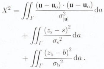
In the above definition of misfit, Γ denotes the area of the finite-element domain (Fig 1), u and u o represent the model and observed surface velocities, respectively, and s and b represent previous estimates of the surface and basal topographies given by the Antarctic folio maps (Reference Drewry,Drewry, 1983). The weighting variables σ|u|, σs and σb are assumed spatially constant and are determined by simple assumptions about the uncertainty associated with the observed surface velocity and previous estimates of surface and basal topography. The purpose of these weighting functions is to normalize the mismatch of each of the three fields according to the uncertainty associated with each field. With this normalization, observations of surface velocity, surface topography and basal topography have equal influence on the determination of τ.
Treatment of observational uncertainty
A particular fit between model and observation is deemed acceptable and the associated estimate of β zs and zb is deemed plausible, when X2 is reduced to a value consistent with random measurement error in the observations of u o, s and b. Measurement error can be characterized by the random vector variable ξ u and the random scalar variables ξs and ξb, which define the deviation of the observed fields from their true values, i.e.
and
where the subscript t signifies the true fields. We assume that the probability distributions of ξu, ξs and ξb are Gaussian and that their means and variances are

where

and

Under the above assumptions, a new positive definite random variable χ2 can be defined:

The probability distribution of this new random variable is known, and is referred to as the χ2 distribution with three degrees of freedom (Reference Menke,Menke, 1989, p. 32).
Our effort to fit model to observation is guided by the assumption that X 2 and χ2 are closely related. In practical terms, we accept a given fit of model to observation and its associated estimate of β, zs and zb , if X 2 is reduced below the bound which χ2 can exceed only with a probability of 10%. The rationale behind this acceptability criterion is that further improvements to the fit would not be differentiated from the effects of random measurement error. This bound is approximately χ2 ≈ 6.25 (Reference Mendenhall, and Schaeffer,Mendenhall and Schaeffer, 1973, p. A32).
An additional unknown which affects ice-stream surface velocity is the flow-law rate constant B involved in the relation between strain rate and deviatoric stress. This constant depends on temperature and crystal fabric. Direct observation of Β is possible only in the laboratory, therefore its variation on Ice Stream Ε must be inferred from assumptions about the temperature distribution and ice fabric of the ice stream. We lack this information, so we are forced either to include B as an unknown variable to he determined by the control method or accept simple assumptions about the variation of B across the ice stream (e.g. that Β is a constant).
As described below, we shall try both strategies in a series of sensitivity tests which provide alternative estimates of β, zs and zb . Experience reveals that lack of uniqueness demonstrated by these sensitivity tests does not bar us from strong conclusions concerning the dynamics of the ice stream and the role of basal friction.
Control-method algorithm
The control method is implemented by an iterative algorithm (see Reference MacAyeal,MacAyeal, 1993a) described as follows. A first guess of the spatial distribution of β, zs and zb , is chosen arbitrarily. This guess is then used with the finite-element model to produce an associated velocity field u. The production of the model velocity field may itself involve several iterations of the model-solution procedure to ensure satisfaction of the flow law.) The model/observation misfit, i.e. u – u 0, is then used to force a model of the adjoint trajectory equations (see Reference MacAyeal,MacAyeal (1993a) for a description of this nomenclature) which produces the vector function Λ. The Λ is then used to evaluate the gradient of X 2 in the space of unknown parameters (i.e. nodal values of the three unknown fields β zs and zb ). A conjugate-gradient method (Reference Press,, Flannery,, Teukolsky, and Vetterling,Press and others, 1989, p. 301) is then used to search for an improved guess of the unknown variables in a direction down the gradient of X 2.
The conjugate-gradient method is an improvement of the steepest-descent method used previously by Reference MacAyeal,MacAyeal (1993a). We use the International Mathematical Sub-routine Library (IMSL) implementation of the conjugate-gradient method provided by the FORTRAN sub-routine UMCGG. The guess-improvement process is repeated many times until X2 converges to a minimum. If this minimum is below the acceptability criterion of 6.25 defined above, the derived β, zs and zb are accepted as being consistent with the observed flow of the ice stream. The derived basal stress τ is then determined from β and u using Equation (1).
Model Description
The control method hinges on use of a numerical model of the ice-stream flow. The two distinctive features of our ice-stream model are: (1) that its horizontal flow is independent of the vertical coordinate z, and (2) that integration of the stress-balance equations over z yields a system of equations that adequately describes this z-independent flow. These simplifications are also used in treatments of ice-shelf dynamics (a discussion of the similarities between ice streams and ice shelves has been offered by Reference MacAyeal,MacAyeal (1989)).
The finite-element model used for this process is constructed from what we assume to be the leading-order approximation of the stress-equilibrium equations considered appropriate for ice-stream conditions (i.e. shallow, incompressible ice sliding over a relatively inviscid layer of basal till, and Glen’s flow law). A justification of this approximation has been given in appendix A of Reference MacAyeal,MacAyeal (1989). The validity of this approximation is contingent on two conditions that deserve special mention. First,

where [B] and [L] are characteristic scales for Β and the horizontal span of the ice stream, respectively. An assumption used to generate this criterion (see Reference MacAyeal,MacAyeal, 1989) is that the characteristic scale representing effective viscosity, [ν], is determined by longitudinal and transverse strain-rate scales [U]/[L] instead of by a vertical-shear strain-rate scale [U]/[H].
For characteristic scales associated with Ice Stream E (listed in the notation section), we see that the first condition, [H]/[L] ≪ 1, is readily met. The second condition, however, can be checked only after the control method has determined τ from the observed fields. Substitution of characteristic scales into Equation (8) requires |τ|≪105Pa Mechanical testing of till acquired from below Ice Stream Β (Reference Kamb,Kamb, 1991; unpublished communication from Reference Engelhardt,, Humphrey,, Kamb, and Fahnestock,Engelhardt and Kamb, 1993) suggests that this condition should be satisfied wherever Ice Stream Ε flows across a deformable basal sediment. We shall see from the results presented below that this condition is met throughout most, but not all, of the ice-stream region Γ. In regions where τ approaches 105Pa, our model breaks down. To correct for this break-down, additional model equations must be developed to account for vertical shear in the horizontal velocity near the bed. Owing to the relatively infrequent occurrence of model break-down in the results presented below, we shall not attempt to correct for vertical shear in the present analysis.
Model equations
The model equations are written

and

where h = zs — zb, g = 9.81 m s−2 is the acceleration of gravity, x and y are horizontal coordinates on a horizontal plane approximating the Earth’s surface (we use a Lambert equal-area projection centered on 90° S) and ρ = 917 kg m−3 is the density of ice (assumed constant).
The model makes use of an effective viscosity υ to represent Glen’s flow law. This representation involves a temperature-dependent rate constant Β and a flow-law exponent n = 3

The velocity in our model is assumed independent of z, thus the rate constant B used in the above expression represents a depth-averaged value of the flow-law rate constant derived from laboratory studies of ice (e.g. Reference Barnes,, Tabor, and Walker,Barnes and others, 1971; Reference Thomas, and MacAyeal,Thomas and MacAyeal, 1982).
Boundary conditions
The boundary condition sufficient for solution of the above equations is u - u 0 at the edges of the finite-element mesh. For further description of the model equations, boundary conditions and their implementation in the control method, we refer to Reference MacAyeal,MacAyeal (1993a). Our specification of velocity as the boundary condition ensures that the stresses at the boundaries are determined as output of the control-method algorithm. This means that aspects of the ice-stream force balance, including the forces transmitted through the sides of the ice stream, are free to vary within the context of fitting the finite-element model to the observed velocity field.
Finite-element algorithm
The finite-element mesh used to cover the study area Γ is shown in Figure 1. This mesh involves 8595 triangular elements (within which fields are linearly interpolated) of variable size and 4563 nodes. Near the edges of the finite-element domain, the mesh resolution is 0.5 km to account for strong gradients in horizontal velocity. In the center of the mesh, the resolution (i.e. the length of a triangular element’s shortest side) is either 2 km or 8 km depending on the density of surface-velocity data points. The regions having the lowest resolution (8 km) are chosen based on the density of velocity-measurement data points. Low resolution in data-poor regions is justified by the need to damp unwanted structure (i.e. wiggles) in the derived fields which cannot be sufficiently constrained by observation.
The finite-element rendition of the forward and adjoint problems described by Reference MacAyeal,MacAyeal (1993a) produced a banded symmetric, positive-definite matrix which is solved using the Cholesky factorization (we used the Lapack software routine SPBTRF on the U.S. National Aeronautics and Space Administration’s Cray C90 sited at Goddard Space Flight Center) and back substitution (Lapack’s SPBTRS).
Observations
To implement the control method, three observed fields are specified in the definition of X 2 (Equation (2)). In addition, the flow-law rate constant B is specified from assumptions about the temperature field. To specify the three observed fields, we interpolate u o, s and b to the finite-element node points. This interpolation involves irregularly distributed observation points and irregularly distributed finite-element nodes. To deal with these irregular distributions, we used the U.S. National Center for Atmospheric Research (NCAR) software routine IDSFFT which triangulates irregularly distributed data and uses quintic polynomial-surface fitting within each triangle. For specification of B, we employed several alternative assumptions about the variation of temperature in the ice stream and conducted a series of sensitivity tests discussed below.
The observed velocity field u o is derived from 32 067 point measurements scattered irregularly across the ice-stream surface (Fig. 1). The computational demands of interpolating these data to the finite-element nodes necessitated using a 6013 point sub-sample of the 32 067 surface-velocity data points. As seen from the Landsat image (Fig. 2), these points are concentrated where displacements of surface features can he identified reliably through comparison of two or more Landsat thematic mapper images (Reference Scambos,, Dutkiewicz,, Wilson, and Bindschadler,Scambos and others, 1992). The variables s and b were derived by digitizing the contours of present-day surface and basal elevation displayed in the Antarctic folio (Reference Drewry,Drewry, 1983) and then interpolating the elevations from the digitized points to the finite-element nodes using the NCAR’s IDSFFT software.
Observational uncertainty
The uncertainties σ|u|, σs and σb are also specified in the definition of X 2. This specification accounts for random measurement error, interpolation error and, in the case of s and b, map-digitization error. For σ|u| we take 6 m a−1, the estimate of standard deviation of point-displacement and image-co-registration errors cited by Reference Bindschadler, and Scambos,Bindschadler and Scambos (1991). Errors associated with s and b are more difficult to estimate. We take σs, = 10 m and σb, = 30 m. These values are consistent with the error analysis of radio-echo sounding surveys of Ice Streams A, Β and C reported by Reference Retzlaff,, Lord, and Bentley,Retzlaff and others (1993).
The error analysis presented by Reference Retzlaff,, Lord, and Bentley,Retzlaff and others (1993) does not apply directly to our problem, because it involves an airborne-radar survey of a different ice stream and with higher spatial resolution than that used to determine s and h in the Antarctic folio maps (Reference Rose,Rose, 1979; Reference Drewry,Drewry, 1983). Our estimates of σs and σb may therefore be too low. However, experience dictates that we accept these low estimates, because σs and σb are also important in characterizing the amplitude of irregularly distributed surface and basal undulations (such as seen in the Landsat image of Figure 2). Such undulations are necessary to achieve a close fit between the model and observed velocity fields. If σs and σb are chosen to be too large, this fit exacts a price of unrealistically rough surface and basal topography. By using the σs and σb values consistent with analysis of undulations reported by Reference Retzlaff,, Lord, and Bentley,Retzlaff and others (1993), we restrict the amplitude of undulations derived by our control method to be similar to that found on Ice Streams A, Β and C.
Results: Standard Inversion
To deal with the uncertain flow-law rate factor B, we ran the control algorithm several times using different assumptions for the variation of Β throughout the ice-stream domain. In one run, we assumed B = 1.73 × 10⁸ to this particular run (run 1) as our standard inversion and use it as a benchmark to which the results of alternative specifications of Β and of other assumptions are compared (Table 1).
Table 1. Comparison of alternative inversions. Results are deemed consistent with observations when X 2 ≤ 6.25. Confidence (%) refers to the chance that random error in the observations could account for a model/observation misfit greater than that associated with the run in question. (Confidence value is defined as the integral of the χ2-distribution with three degrees of freedom from the X 2 value listed in column 3 to ∞.)

The assumption that
Another factor, which motivates the choice
The minimum value of X 2 achieved for the standard inversion was 4.26, well below the 6.25 acceptability criterion suggested by our consideration of random measurement errors (Table 1). The probability that χ2 (Equation (7) exceeds X 2 = 4.26 is 23% (Table 1), thus model/observation mismatch attained by the standard inversion is consistent with the effects of random error in the observed fields, As shown in Table 2, the spatial average of velocity mismatch, |μ–μ o|, is 8.7 m a−1 This value is comparable to the standard deviation estimated for the velocity measurements σ|μ o|=6 m a–1.
Table 2. Statistics of standard inversion (run 1)

Derived fields
Derived fields associated with our standard inversion are displayed in Figures 3–7 along with the data used to generate them. A statistical summary is presented in Table 2. A close-up view of the derived fields for a limited 47 km by 33 km region covering the middle section of the ice stream is displayed in Figure 8 (see Figure 7 for the location of this sub-region).

Fig. 3. Observed surface-velocity magnitude |uo| (left), model surface-velocity magnitude (right) (c.i. 50 m a−1) derived from the standard inversion.

Fig. 4. Velocity misfit |u — uo| for the standard inversion. The standard deviation of observed velocity error is approximately 6 m a−1.

Fig. 5. Surface topographies. Previous estimates (left), result of standard inversion zs (right) (c.i. 50 m).
Sticky spots
The basal-friction field derived by our standard inversion (Fig. 7) displays the result we expected from previous study (Bindschsdler and Scambos, 1991; Reference MacAyeal,MacAyeal, 1992); namely, that basal friction is dominated by an irregular distribution of basal sticky spots. (We do not show a map of the basal-coupling parameter β2, because of its similarity in appearance to the map of |τ|.) To emphasize this irregularity, we give area-distribution functions and cumulative area-distribution functions of |τ| and β2 in Figures 9 and 10. The relative importance of basal stress in resisting; the local driving stress is also shown in Figure 9. A comparison of the area-distribution functions associated with |τ| and pgh|∇zs | indicates that basal stress eaten a weds wider range of variation than the driving stress and is, on average, smaller in magnitude than the driving stress. This indicates that horizontal deviatoric-stress gradients are an important resistive element in the force balance of the ice stream. Approximately 30% of Γ possesses a basal stress less than 103 Pa. This result is consistent with the widespread presence of deformable basal till as a lubricant beneath the ice stream (Reference Kamb,Kamb, 1991). Sticky spots, taken here to be regions where |τ| exceeds 5 × 10⁴Pa, comprise about 15% Γ.

Fig. 6. Basal topographies. Previous estimate b (left), result of standard inversion zs (right) (c.i. 50 m).

Fig. 7. Derived |τ| (Pa) from the standard inversion. Magnitudes less than 10 Pa are denoted by clear (white) color. Box indicates sub-region shown in detail in Figure 8.
The area-average of |τ| in the standard inversion is 1.41 × 10⁴Pa (Table 2). The area-average driving stress is 4.87 × 10⁴Pa. Thus, on average, about 29% of the driving stress is balanced by basal friction. The role of basal stress in balancing driving stress in this general sense remains somewhat uncertain because our knowledge of flow-law rate parameter variation is limited. The sensitivity experiments described in the following sections consider alternative specifications of Β and provide some sense of the uncertainty of the area average of |τ| (i.e. ±103 Pa; Table 3). These sensitivity experiments do not explore the uncertainty generated by systematic variations of Β that could accompany strain heating and crystal-fabric development in the shear margins of the ice stream.
Ice softening in shear margins has been studied by Reference MacAyeal,(MacAyeal 1989; see Table 2 and Figure 11 of this reference) in the context of Ice Stream B. MacAyeal’s sensitivity experiments using the same finite-element model as that used here indicate that ice softening by a factor of 10 could increase the horizontal velocity of Ice Stream Β by a factor of 2. This result implies that our 29% figure for the proportion of driving stress balanced by basal stress is a lower bound. A reasonable guess of the upper bound based on MacAyeal’s (1989) sensitivity experiments is 60%. At present, we do not pursue this question further because we believe that a reliable answer can be reached only when more accurate surface and basal topography data are available, shear margins are better resolved m the velocity data and model physics can account for conditions where [H]/[L] ≈ 1 at the ice stream sides.
Table 3. Effect of flow-law rate constant an derived basal friction

Sticky spots in some regions appear to be linked into narrow bauds several tens of kilometers in length and only several kilometers in width. We call these features sticky strings. We have no explanation for sticky strings. In some circumstances, they correspond with surface lineations visible in Landsat imagery (e.g. the linear features which cut obliquely across the Landsat image in Figure 2). A possible explanation of this correspondence is that structure in the bedrock serves to generate an efficient basal-water conduit which locally decreases the water pressure at the ice/bed contact and within pores of the subglacial sediment (personal communication from R. C. A. Hindmarsh, 1993). Such a decrease would be expected to make the ice/bed contact more rigid and lead to a sticky string aligned with bedrock structure.
To examine our results for the suggestion of a basal-sliding law, we present in Figure 11 a scatter plot of |u| vs |τ| where each point represents conditions in one of the 8595 triangular elements. The lack of coherent structure in Figure 11 suggests that basal friction is not a simple function of ice velocity such as would be the case if the subglacial bed could be idealized as a subglacial till of uniform viscosity and thickness. Our results suggest that the essential physical controls on the basal friction of Ice Stream Ε (e.g. water pressure) have yet to be determined.
Test of model assumptions
As shown in Table 2, the area-average of |τ| in the standard inversion is 1.41 × 10⁴Pa. This value is relatively small compared to the criterion [τ] ≪ 105 which justifies the assumptions on which our treatment of ice-stream dynamics is based. We therefore regard our model as satisfying the relationship expressed in Equation (8) in a large-scale, average sense.

Fig. 8. Detail of derived results of standard inversion for sub-region indicated by the box in Figure 7. The dimensions of this sub-region are 47 km by 33 km. Basal stress magnitude |τ| (panel a), model velocity magnitude |u| (panel b) (c.i. 20 m a−1), derived basal topography Zb (panel c) (c.i. 50 m), velocity misfit |u — uo| (panel d) (c.i. 20 m), observed surface-velocity magnitude (panel f) (c.i. 20 m a−1).
The maximum local value of |τ| produced by our standard inversion, however, is 2.19 × 10⁵ Pa and is not small compared to the criterion [τ] ≪ 105 which justifies the assumptions on which our model is based. The results of our standard inversion are therefore not consistent with the assumptions used to generate them in several limited regions surrounding the strongest sticky spots. In view of the limited extent of these regions and the close agreement between model and observed velocity attained generally throughout the ice stream, we choose to accept model errors generated by this inconsistency and defer further consideration of such errors to some future study in which the small-scale flow variation near a particular sticky spot where |τ| exceeds 105 Pa is of concern.

Fig. 9. Area-distribution function (upper) and cumulative area-distribution function (lower) for |τ| and pgh|∇zs| determined by the standard inversion. The value of the area-distribution function (upper) for a given stress magnitude expresses the fraction of total ice-stream area which possesses a basal traction or driving stress within a small range of the given stress. The size of the stress range is variable and is designed to cover the range between 1 and 106 Pa with 100 intervals of equal length on a logarithmic scale. The value of the cumulative area-distribution function (lower) for a given stress represents the fraction of total ice-stream area which possesses a basal traction or driving stress with a magnitude less than the given stress.
Surface and basal topography
As expected, zs and zb , derived from our standard inversion displays roughness with characteristics similar to roughness found on Ice Stream Β (Reference Retzlaff,, Lord, and Bentley,Retzlaff and others, 1993) (Figs 5 and 6). In the sub-region shown in Figure 8 (panels c and e), zs tends to intensify over a site of increased basal friction. Examination of other regions suggests that surface-slope steepening can also occur over bumps in basal topography which may lack strong basal friction. No account is made of mass-balance considerations in this study. It is therefore possible that the relationship between surface topography, basal topography and horizontal flow derived here may be inconsistent with steady state. Further analysis of this question is deferred to the future when more accurate observations of s and b may become available through satellite altimetry and additional radio-echo sounding.
Simulated satellite image
An independent assessment of the quality of our standard inversion is made by examining the correspondence between surface features seen in the Landsat image (Fig. 2) and surface features associated with zs . Simulated satellite images of both the derived surface topography zs and the previous estimate s are given in Figure 12. The simulated images were constructed from the surface slope in the direction roughly parallel to the Sun azimuth of the Landsat image (Fig. 2). These images were then smoothed to reduce the prismatic visual appearance (i.e. constant gray level in each triangular element) introduced by the finite-element discretization.

Fig. 10. Area-distribution function (upper) and cumulative area-distribution function (lower) for β2 derived by the standard inversion. See the caption of Figure 9 for an explanation of the meaning of these functions.

Fig. 11. Points represent average values of |τ| and |u| for the standard inversion in each of the 8595 elements comprising the finite-element mesh
The most striking resemblance between the Landsat image (Fig. 2) and its simulated counterpart of zs (Fig. 12) is the general mottled appearance due to small-scale undulations. The apparent basal escarpments which slash obliquely across the ice stream’s mid-section in the Landsat image appear to have counterparts in the simulated image of zs . In the simulated image, these oblique linear features are associated with steps in the ice-stream surface above sticky strings at the root of the obliquely slashing features in the real Landsat image.

Fig. 12. Simulated satellite images associated with the previous estimate of surface topography s (left) and the surface topography resulting from the standard inversion zs (right). These images represent gray-scale renderings of -∂s/∂y and -∂zs/∂y where y is the horizontal coordinate which runs vertically (positive upward) in the map plane. Brightness of the images corresponds to illumination from the positive y direction and is approximately equivalent to the Sun angle of the Landsat image in Figure 2. The images were smoothed to eliminate patchiness associated with the finite-element discretization. Wide boundaries of relatively uniform color at the edges of the active finite-element domain are artifacts of the smoothing algorithm. A linear feature indicated by the arrow in the image of the model surface corresponds in position and geometry with the prominent linear feature of the real Landsat image displayed in Figure 2.
In contrast with the simulated image of zs , the simulated image of s bears little resemblance to the real Landsat image. We regard the appearance of the simulated image of zs to be more realistic than that of s, and interpret this realism as an independent check on the results of our standard inversion.
Results: Alternative Inversions
The control algorithm was run through several additional inversions of the data to test alternative assumptions. The minimum X 2 values obtained for these alternative inversions are compared with that of our standard inversion in Table 1. In some cases, results associated with given alternative assumptions yield X2 values greater than the 6.25 acceptability criterion. The assumptions used to generate these results are therefore rejected. In cases where X 2 is less than 6.25, results and associated assumptions are considered equally plausible as those of our standard inversion. These cases illustrate the non-uniqueness of solutions of the ice-stream force-balance inverse problem.
Relative importance of basal friction, surface topography and basal topography
A crucial sequence of alternative inversions (runs 2–4) were run to examine the question of whether variation in any or all of the three fields β, zs and zb could be arbitrarily replaced with a simple, intuitively motivated prior estimate (i.e. a guess) without significantly altering the fit between model and observed surface velocity. In these runs,
In run 2, we computed X 2 under the assumption that the control method provides no added value to the prospect of fitting model to observation, i.e. that a good guess of the unknown fields would be sufficient. For this guess, we take β = 1.67 × 10⁴ (Pa m s−1)½, zs = s and zb , = b. The uniform value of β for this run is the area average of the β field derived in our standard run (Table 2). As indicated by its associated X 2 value (Table 1), the hypothesis tested by run 2, i.e that a good guess of unknown ß, zs and zb , is sufficient, is false.
In runs 3 and 4, we tested the assumptions that the observed velocity field could be explained, in the first case, without basal friction (β = 0) and, in the second case, without adjustments of surface and basal topography from their previous estimates (zs = s and zb = b). Again, the X 2 values obtained for these runs rule out their associated hypotheses. We are therefore forced to conclude that spatial variability in basal friction, surface topography and basal topography are equally important influences on the surface velocity of Ice Stream E. This result motivates additional future measurements of surface and basal topography that may be possible using satellite altimetry and additional airborne radio-echo sounding.
Flow-law rate-factor variation
To examine the consequences of flow-law rate-factor uncertainty, we present runs 5-8. In run 5, we assume ice to be a viscous fluid with constant viscosity ν = 1014 Pa s. In runs 6 and 7 we use uniform Β with values of 1.5 and

Fig. 13. Area-distribution functions (upper) and cumulative area-distribution functions (lower) for |τ| for runs with various treatments of the flow-law rate factor Β (runs 1 and 6–8). See the caption of Figure 9 for an explanation of the meaning of these functions. Similarity among the functions plotted here suggests that uncertainty in the specification of Β does not affect the derived τ in a qualitatively important way.
Run 5 was found to be incompatible with the observations (Table 1). A linear viscous flow law is therefore ruled out and a non-linear (e.g. power) flow law is found to be mandatory. Runs 6 and 7 were found to be compatible with observations (Table 1). These runs, plus our standard inversion

In run 8, we employ the control method as a means to select a variation of B, in addition to the other three unknown fields, to fit the data better. In this circumstance, we add an additional term to X 2 as follows

where
A map of Β determined in run 8 is displayed in Figure 14. The area-distribution function and cumulative area-distribution function of B are displayed in Figure 15. The pattern of Β derived in run 8 has greater variability in regions where velocity data points are sparse. We are therefore tempted to conclude that this pattern is determined primarily by errors in the velocity data.
Basal drag tied to bumps in basal topography
Reference Alley,Alley (1993) suggested that sticky spots may be caused by large bedrock bumps which stick into the base of the ice stream or which compromise an intervening layer of a lubricating substance such as water or basal till. The results of our standard inversion (run 1) were generated under the assumption that zb and β2 were completely independent. A scatter plot of elemental values of zb vs β2 (not shown) derived from our standard inversion fails to suggest a relationship between β2 and zb . The observations we invert therefore support an hypothesis that zb and β2 need not be related. This does not mean that the observations we invert definitively rule out such an hypothesis.

Fig. 14. Variable, flow-law rate factor Β (Ρa s1/3 ) derived by run 8.

Fig. 15. Area-distribution function (upper) and cumulative area-distribution function (lower) for Β derived by run 8. See the caption of Figure 9 for an explanation of the meaning of these functions.
To examine Alley’s suggestion further, we ran run 9 under the assumption

where S = 5.0 × 10⁹ Pa s. We require the perturbation of the basal elevation above its previous estimate b to be positive and to have an amplitude of σb, = 30 m when the bed-coupling parameter β2 rises to approximately half of a representative sticky-spot value (i.e. 5 × 10⁹ Pa s). The hypothetical relationship expressed in Equation (13) is arbitrary and bears little resemblance to the scale analysis presented by Reference Alley,Alley (1993).
For run 9, X 2 < 6.25; thus, the relationship represented by Equation (13), and presumably many other such relationships which tie β2 to zb , is consistent with the observations. This result, in concert with the results of the standard inversion where β2 to zb , were assumed independent, suggests that our analysis is unable to resolve the question of how basal friction should relate to basal topography. This question perhaps can be answered when more accurate observations of s and b become available.
Conclusion
Comparison with previous results
Our results confirm previous suggestions that basal shear stress of the West Antarctic ice streams is extremely low (< 104 Pa) except in isolated sticky spots (Reference Kamb,Kamb, 1991). These characteristics are compatible with the notion that soft, unconsolidated sediments lubricate the base of the ice stream. Our results further suggest that sticky spots, not intervening lubricated zones which are nearly stress free, appear to determine the overall contribution of basal friction to the forces which resist ice-stream discharge. While significant in the overall force budget of the ice stream, friction induced by sticky spots is not, however, the dominant resistive stress. Drag introduced at the ice-stream’s sides and at the grounding line (i.e. ice-shelf back-pressure) are also significant resistive forces. We therefore suggest that the question which is most important, basal friction or side and grounding-line drag, has no definitive answer. Both can be important.
The pattern and location of sticky spots we find in our standard inversion suggest that bedrock topography, rock type or large-scale structure such as faults or escarpments which affect water pressure can cause sticky spots below ice streams. This suggestion is in agreement with theory (Reference Alley,Alley, 1993) but a further test of theory is beyond the resolving power of our methods and data. We therefore suggest that additional measurements, perhaps involving satellite-altimeter profiling, airborne-radar sounding and passive seismology (e.g. Reference Anandakrishnan, and Bentley,Anandakrishnan and Bentley, 1993), be focused in small-scale regions where sticky spots appear on Ice Stream E.
Previous studies of ice-stream force balance (Reference Whillans, and van der Veen,Whillans and Van der Veen, 1993; Reference Whillans,, Jackson, and Tseng,Whillans and others, 1993) failed to find direct evidence for sticky spots on Ice Stream B. We do not consider our results to be incompatible with conditions found on Ice Stream B. The study areas on Ice Stream Β which appear to lack sticky spots are comparable in size with some of the sticky-spot-free zones found near the grounding line of Ice Stream Ε (e.g. as suggested by Figure 7).
Lessons for ice-stream modeling
Our results suggest that basal friction below ice streams is not determined by purely glaciological considerations. We suspect that basal friction depends crucially on the interplay between ice conditions, geologic properties of the bedrock, subglacial hydrologic conditions and the disposition of unconsolidated basal sediments. Up to now, ice-sheet modelers have attempted to rely on various basal-sliding laws as a means to characterize ice-stream flow (e.g. Reference Bentley,Bentley, 1987). The simplest of these laws express τ as a function of basal-ice velocity. Our results suggest that these simplest laws may oversimplify. The origin of sticky spots may depend as much on the geophysical properties and history of the glacial bed as with the ice stream above. Our results suggest that the intricate pattern of basal coupling that controls the present flow of ice Stream E arises from some as yet inscrutable property of the bed that escapes our understanding. Ice-stream modelers are urged to heed signs of this inscrutability and to recognize the virtue of simple basal-sliding laws that mimic the statistics of conditions found below Ice Stream E.
Acknowledgements
We thank I. Whillans, R. Hindmarsh and R. Alley for valuable discussions on early drafts of this paper. J. Glen, K. Hutter and an anonymous referee provided suggestions which ultimately led us to achieve far more satisfying results with the control method than were originally displayed on an initial draft of this paper. T. Dupont helped to assemble data and figures used in this study. P. Vornberger provided the Landsat images shown in Figure 2. Financial support was provided by the National Aeronautics and Space Administration (NASA) grant NAGW 2588, and by the U S. National Science Foundation (NSF) grants OPΡ 9218078 and OPP 9321457. Computer support was provided by NASA’s Goddard Space Flight Center, in particular the NASA Center for Computational Sciences.


