


1. Introduction
Thanks to the excellent propagation characteristics of electromagnetic waves in snow and ice, ground-penetrating radar (GPR) has been one of the key geophysical methods used in the field of glaciology for over 50 years (Schroeder and others, Reference Schroeder2020, Schroeder, Reference Schroeder2022). Initially developed and tested in polar regions (e.g. Harrison, Reference Harrison1970; Jacobel and Anderson, Reference Jacobel and Anderson1987; Bamber, Reference Bamber1989), GPR is now employed regularly on alpine glaciers worldwide to (i) determine ice thickness and estimate ice volume (e.g. Narod and Clarke, Reference Narod and Clarke1994; Fountain and Jacobel, Reference Fountain and Jacobel1997; Flowers and Clarke, Reference Flowers and Clarke1999); (ii) monitor the nature of the glacier bed and identify sedimentary structures (e.g. Arcone and others, Reference Arcone, Lawson and Delaney1995; Glasser and others, Reference Glasser, Goodsell, Copland and Lawson2006; King and others, Reference King, Smith, Murray and Stuart2008); (iii) identify shear zones and crevasses (e.g. Goodsell and others, Reference Goodsell, Hambrey and Glasser2002; Nobes and others, Reference Nobes, Davis and Arcone2005; Bradford and others, Reference Bradford, Nichols, Harper and Meierbachtol2013); (iv) map internal water bodies and subglacial lakes (e.g. Vincent and others, Reference Vincent2012; Garambois and others, Reference Garambois, Legchenko, Vincent and Thibert2016; Rutishauser and others, Reference Rutishauser2022); (v) estimate ice water content (e.g. Pettersson and others, Reference Pettersson, Jansson and Blatter2004; Murray and others, Reference Murray, Booth and Rippin2007; Bradford and others, Reference Bradford, Nichols, Mikesell and Harper2009); (vi) distinguish between cold and temperate ice (e.g. Brown and others, Reference Brown, Harper and Bradford2009; Eisen and others, Reference Eisen, Bauder, Lüthi, Riesen and Funk2009; Bælum and Benn, Reference Bælum and Benn2011); (viii) identify and characterize englacial and subglacial channels (e.g. Sharp and others, Reference Sharp1993; Moorman and Michel, Reference Moorman and Michel2000; Kulessa and others, Reference Kulessa, Booth, Hobbs and Hubbard2008); and (viii) study glacier surge mechanisms (e.g. Jacobel and Raymond, Reference Jacobel and Raymond1984; Murray and others, Reference Murray2000; Woodward and others, Reference Woodward, Murray, Clark and Stuart2003).
Typically, GPR surveys conducted on glaciers have involved the acquisition of data over one or a small number of profile lines (e.g. Farinotti and others, Reference Farinotti, Huss, Bauder, Funk and Truffer2009; Harper and others, Reference Harper, Bradford, Humphrey and Meierbachtol2010; Urbini and others, Reference Urbini2017), thus providing a 2D transect view of the englacial and subglacial conditions. Over the past decade, an increasing number of researchers have carried out so-called 3D GPR surveys in alpine glaciological environments, where data are acquired over a series of regularly spaced parallel survey lines to gain further detailed information about the internal structure of the ice and/or bed geometry (e.g. Saintenoy and others, Reference Saintenoy2013; Langhammer and others, Reference Langhammer, Grab, Bauder and Maurer2019b; Egli and others, Reference Egli, Irving and Lane2021a). In this regard, both ice-based (e.g. Binder and others, Reference Binder2009; Saintenoy and others, Reference Saintenoy2011; Del Gobbo and others, Reference Del Gobbo, Colucci, Forte, Triglav Čekada and Zorn2016) and helicopter-based (e.g. Merz and others, Reference Merz, Green, Buchli, Springman and Maurer2015; Rutishauser and others, Reference Rutishauser, Maurer and Bauder2016; Grab and others, Reference Grab2018) 3D GPR surveys have been conducted. On one hand, ice-based surveys allow for the acquisition of high-density and high-resolution 3D GPR data and have proven to be a valuable tool for the study of, for instance, englacial and subglacial hydrology (Church and others, Reference Church2019; Church and others, Reference Church, Bauder, Grab and Maurer2021; Egli and others, Reference Egli, Irving and Lane2021a). However, the corresponding data acquisitions are labor intensive and slow to carry out, and the surveyed areas are consequently limited in size. Such surveys may also be dangerous due to surface features such as crevasses and moulins, or even impossible in regions of the glacier that are inaccessible. Helicopter-based surveys, on the other hand, permit the coverage of larger areas (e.g. Arcone and Yankielun, Reference Arcone and Yankielun2000). However, in addition to being expensive and polluting, they come at the cost of reduced resolution of internal glacier structures as the GPR antennas are located much further from the ice surface. Further, helicopter-based survey lines cannot be flown with a spacing on the order of the dominant GPR wavelength in order to provide high-density measurements.
Repeated 3D GPR acquisitions over the same area, otherwise known as 4D surveys, are even less common in glaciological settings. Indeed, with such acquisitions, the above-listed drawbacks become even more determinant and there exists the additional challenge of returning to the glacier on a regular basis to record 3D GPR data in the same spatial locations. Nonetheless, previous initial work has suggested that time-lapse GPR measurements on glaciers may be valuable. Irvine-Fynn and others (Reference Irvine-Fynn, Moorman, Williams and Walter2006), for example, examined the hydrothermal dynamism within a polythermal glacier during a single ablation season and showed that the ice water content varies in response to an evolving englacial and subglacial drainage system. Church and others (Reference Church, Grab, Schmelzbach, Bauder and Maurer2020) mapped the spatial extent of a dynamic englacial conduit network on a temperate glacier multiple times over a two-year period, which provided insight into the evolution of the glacier hydrological system. Finally, Mingo and others (Reference Mingo, Flowers, Crawford, Mueller and Bigelow2020) detected changes in englacial water storage using time-lapse GPR surveys, which led to a better understanding of englacial lake filling and drainage cycles. All of this research leads us to expect that recording frequent high-resolution and high-density repeated 3D GPR data on glaciers would provide new and important insights into glacier temporal dynamics. At the present time, however, a means of acquiring such data over relevant areas of interest and reasonable time frames does not exist.
In recent years, numerous advances in uncrewed aerial vehicle (UAV) or drone technology have opened new and exciting data acquisition possibilities in the field of geophysics. Indeed, a wide variety of geophysical instruments have been deployed on drone-based platforms, which include: (i) electromagnetics (e.g. Stoll and others, Reference Stoll2019; Parshin and others, Reference Parshin2021; Kotowski and others, Reference Kotowski2022), (ii) magnetics (e.g. Døssing and others, Reference Døssing2021; Kolster and Døssing, Reference Kolster and Døssing2021; Walter and others, Reference Walter, Braun and Fotopoulos2021), (iii) gamma-ray (e.g. van der Veeke and others, Reference van der Veeke2021a; van der Veeke and others, Reference van der Veeke, Limburg, Koomans, Söderström and van der Graaf2021b; Kunze and others, Reference Kunze2022), (iv) gravity (e.g. Weiner and others, Reference Weiner2020; Luo and others, Reference Luo2022), (v) lidar (e.g. Lin and others, Reference Lin2019; Yin and Wang, Reference Yin and Wang2019; Tao and others, Reference Tao2022), (vi) sonar (e.g. Dietrich, Reference Dietrich2017; Bandini and others, Reference Bandini2018; Koutalakis and Zaimes, Reference Koutalakis and Zaimes2022) and (vii) radar instruments. Initial drone-based radar systems involved small, lightweight antennas, first operating in the Ka-band (24–40 GHz) (Weiss and others, Reference Weiss and Ender2005), followed by the X-band (8–12 GHz) and C-band (4–8 GHz) (Zaugg and others, Reference Zaugg2010; Remy and others, Reference Remy, de Macedo and Moreira2012; Aguasca and others, Reference Aguasca, Acevo-Herrera, Broquetas, Mallorqui and Fabregas2013). These systems proved that radar imaging using UAVs is feasible but were not suitable for subsurface investigations due to the limited penetration into the ground. Subsequent systems permitted operation at lower frequencies and were sufficiently advanced to be used in the context of (i) landmine detection (Burr and others, Reference Burr2018; Fernandez and others, Reference Fernandez2018; Dill and others, Reference Dill, Schreiber, Engel, Heinzel and Peichl2019); (ii) archeological exploration (Yarleque and others, Reference Yarleque, Alvarez and Martinez2017); (iii) snow cover investigation (Jenssen and others, Reference Jenssen and Jacobsen2020; Jenssen and Jacobsen, Reference Jenssen and Jacobsen2020); (iv) soil moisture mapping (Wu and others, Reference Wu2019); (v) snow hydrology (Valence and others, Reference Valence, Baraer, Rosa, Barbecot and Monty2022); and (vi) avalanche rescue (SPH Engineering). An excellent review of the state-of-the-art of contactless GPR imaging, specifically with regard to UAV-borne GPR, is presented in Catapano and others (Reference Catapano2022). In all of the above cases, however, the developed GPR systems involved antenna frequencies ranging from 500 MHz to 4 GHz which still do not allow for sufficient penetration into a glacier. To our knowledge, a drone-based GPR instrument operating at lower frequencies, with the specific objective of investigating internal glacier structures in detail, has not yet been presented.
In this paper, we introduce a newly developed drone-based, impulse GPR system that has been designed for the specific purpose of conducting high-density 3D and 4D surveys on alpine glaciers in a safe and highly efficient manner, thereby combining the advantages and minimizing the disadvantages of ice-based and helicopter-based surveys. The system takes advantage of modern real-time-sampling GPR technology with a high number of stacks, which permits the rapid collection of high-resolution data. A single custom-made transmit–receive antenna, operating at a center-frequency of 80 MHz, along with carbon-fiber supports ensure a minimal payload weight, thus maximizing flight time on a single set of batteries. Drone flight localization using dGPS technology permits the precise following of parallel survey lines, which is essential for the acquisition of high-quality 3D and 4D data. We first outline below the drone-based GPR system and data acquisition methodology. Next, we describe a series of flight parameter tests performed to optimize the system stability and quality of the measurements. Finally, to illustrate the potential for drone-based GPR on glaciers to acquire large high-density and high-resolution 3D data, we present a recently recorded dataset from the Otemma glacier, Switzerland.
2. The drone-based GPR system
2.1. Construction and specifications
Our drone-based GPR system is divided into four different units (Fig. 1). The Drone Unit is comprised of an M300 RTK drone manufactured by Shenzhen DJI Sciences and Technologies (China) along with the True Terrain Following (TTF) navigation system developed by SPH Engineering (Latvia). The GPR Unit contains a GPR controller, which was custom designed to our specifications by Utsi Electronics Ltd. (UK), and a homemade single transmit–receive antenna, both of which are connected to the Drone Unit using custom designed 3D printed parts. The Operator Unit is composed of a field computer, a mobile phone, as well as a remote controller for the drone. Finally, the dGPS Unit consists of the D-RTK 2 high-precision global navigation satellite system (GNSS) mobile station from DJI.

Figure 1. Drone-based GPR system: (a) illustration of the system components; (b) diagram showing the structure and interactions between the devices; (c) photo of the system operating over the Otemma glacier in August 2022.
The M300 drone, when used in real time kinematic (RTK) mode with the D-RTK 2 base station, has a navigational positioning accuracy of approximately 1 cm horizontally and 2 cm vertically thanks to real-time differential GPS corrections. When combined with the TTF system, which is composed of an onboard computer and a 24-GHz radar altimeter, it can correct its elevation as it flies with the aim of keeping an approximately constant height above the glacier surface. This function is particularly important in areas where the surface topography is highly variable in the sense that we wish to fly as close to the glacier as practically possible in order to optimize the resolution of the GPR data. Flight parameters, such as the desired height of the drone above the surface or the maximum descent speed, are set via an internal configuration file. Additionally, GPS data are output from the drone to the GPR controller such that each GPR trace is tagged with its exact time and position. All flight data, including the drone speed, flight dynamics parameters (i.e. pitch, roll and yaw angles), dGPS positions and RTK status, are logged while the system is in operation.
The GPR controller is responsible for both generating the radar pulse that is sent into the antenna and recording the pulses that are reflected from heterogeneities within the ice. Sampling of the recorded waveform is done in real time, meaning that each GPR trace is recorded all-at-once rather than through a series of interleaved samples. Each trace is thus stored rapidly, which means that many stacks are possible and that a high signal-to-noise ratio can be achieved. Indeed, our GPR controller records 24-bit traces over a time range of 2800 ns, corresponding to a survey depth of more than 200 m in glacier ice, with a temporal sampling interval of 3.125 ns. The trace acquisition rate is approximately 14 Hz and each raw measurement is stacked roughly 5000 times, resulting in an expected 70-fold improvement of signal-to-noise. When flying the drone at a speed of 4 m s−1, we are able to record more than three GPR traces per meter, which allows for high-quality along-profile data. Our custom-built lightweight unshielded GPR antenna, used in monostatic mode, is a resistively loaded butterfly dipole having a center frequency of approximately 80 MHz and an effective bandwidth of 120 MHz. With this antenna, we have found that we can typically image to well over 100 m depth in temperate alpine glaciers, even in regions where substantial rock debris is present on the glacier surface. Finally, GPS NMEA sentences are logged by the GPR controller at a rate of 5 Hz such that the position of each GPR trace can be precisely determined. Data are recorded onto an SD card located on the controller in order to avoid interference with the radio command. Recording of GPR data begins immediately when the system is turned on.
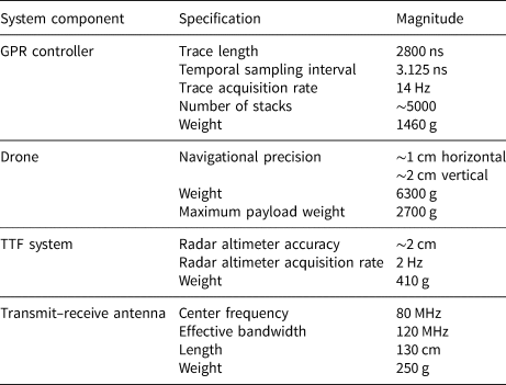
Table 1 summarizes the specifications of the different components of the drone-based GPR system along with their weights. The total payload of the system is approximately 2.2 kg, which is well below the 2.7 kg payload capacity of the M300 drone. According to the manufacturer, the flight time of the M300 on a single set of batteries with such a payload should be approximately 34 min. However, this is highly variable and depends not only on the survey conditions (e.g. air temperature, pressure, wind speed), but also on the flight parameters discussed in Section 3.1.
Table 1. Drone GPR system specifications
2.2. Survey methodology
The first step in conducting a drone-based GPR survey is planning the flight mission. This is done either in advance at the office, or on-site in the field, and is accomplished using the Universal ground Control Software (UgCS) software from SPH Engineering. To this end, we use the so-called Area Scan tool to define a series of parallel survey lines over the region of interest. This involves choosing the desired orientation of the lines, the orientation of the drone, the line spacing and the flight speed. With this information, the software then programs a succession of waypoints to which the aircraft will fly in chronological order.
After planning the flight mission, its feasibility is verified using a smaller and cheaper ‘crash drone’ before conducting the final 3D GPR survey. Indeed, even if the M300 drone has anticollision sensors on all sides, highly variable topography including a rough glacier surface, steep valley walls, lateral and medial moraines, and the presence of large boulders represents a difficult flight environment, and all efforts are made to ensure that a crash with expensive geophysical equipment is avoided. Further, the survey environment may change during a 4D survey, in the sense that glacier melt between acqusitions may put the boundaries of the GPR grid closer to valley walls than in previous surveys. As the smaller drone will not have the battery capacity to fly the entire grid, a second mission is created whose primary purpose is to check the edges of the survey domain as well as any visibly challenging regions in its interior. We have found this strategy to be sufficient to ensure the safety of the system.
Once the flight mission has been correctly programmed, the D-RTK 2 base station is configured. When considering 4D GPR surveys and to ensure the best possible mission repeatability in terms of positioning, the base station should be placed at the same location for each acquisition. The mission is next uploaded to the remote controller, and the TTF mode is activated using a second software, the UgCS Custom Payload Monitor (CPM). Once the mission has started, the drone moves toward the first waypoint of the trajectory, orients itself as programmed, and begins to fly along the first profile. Because the flight missions are generally significantly longer than what the system can cover using a single set of drone batteries, the batteries must be changed during the survey. In this regard, when the batteries reach a critically low level (minimum 20%), the mission is paused and the drone is landed manually. After changing the batteries, the mission is uploaded again from the last waypoint reached in the previous flight and the data acquisition is resumed. In the common case where the drone needs to be flown back to the operator because its location on the glacier is difficult to access, the mission must be stopped earlier to dedicate battery power to that task.
3. Flight parameters and testing
In the following we explore the effects of various flight parameters for the drone-based GPR system with the aim of optimizing its performance. We first consider different types of turns and mission trajectories and their impact on the flight path, drone battery consumption and survey logistics. We then address the choice of profile line spacing for 3D and 4D alpine glacier surveys. Next, we examine the effect of the chosen flight speed and height above the glacier surface on survey logistics and GPR data quality. Finally, we assess the stability of the system during data acquisition.
3.1. Turns and trajectories
The UgCS software proposes two options for turning the drone after the completion of each profile line: the Stop & Turn (S&T) and the Adaptive Bank Turn (ABT) (Fig. 2). With the S&T option, the drone flies directly to each waypoint, stops, and then moves towards the next waypoint. In this manner, the turns are abrupt. Conversely, with the ABT option, the system considers that it has reached a particular waypoint when it comes within a prescribed acceptance radius. It begins moving towards the next waypoint without stopping its motion, and in this manner the turns are smooth. Both types of turns were tested to assess their impact on the quality of the resulting flight paths and on the battery consumption. To this end, a flight trajectory comprised of twenty-six, 105-m-long profile lines, laterally spaced by 2 m, was programmed and flown at a specified speed of 3 m s−1. The profiles were flown in sequential order from one side of the grid to the other. Figures 3a and b show the path taken by the drone and the measured flight speed using the S&T and ABT options, respectively. As expected, we see that the S&T option results in straighter flight lines, whereas the ABT option results in slight deviations from the scheduled trajectory when starting a new profile. Further, the flight speed along each profile line is more uniform using S&T turns which translates into a more constant GPR trace acquisition rate in distance. The drone battery consumption during the S&T test, however, was found to be 64%, whereas it was 41% for the ABT test, which represents a 23% difference. Battery life being most critical in our case, it was decided to always use the ABT option with the drone-based GPR system. Issues related to variable drone speed along the GPR survey lines and slight deviations from the programmed path are indeed relatively minor and can be addressed by careful binning of the data (see Section 4.3).

Figure 2. Two types of turns available with the UgCS software. S&T: Stop & Turn. ABT: Adaptive Bank Turn. WP: Waypoint.

Figure 3. Drone position and speed for two types of turns and trajectories: (a) Stop & Turn option for a trajectory where the GPR profile lines are flown in sequential order (drone battery consumption 64%); (b) Adaptive Bank Turn option for the same trajectory as in (a) (drone battery consumption 41%); (c) Adaptive Bank Turn option for a trajectory where the odd-numbered profiles are flown first in sequential order, followed by the even-numbered profiles in reverse order (drone battery consumption 40%). The programmed drone speed was 3 m s−1.
Even when using the ABT option, the drone still needs to decelerate and accelerate strongly when moving from one profile to the next, and an important part of its battery consumption is dedicated to these transitions. To mitigate this issue, one might consider modification of the flight trajectory in order to increase the turn radius at the expense of not flying the profiles in sequential order. The latter is common in marine bathymetry surveys where it is not possible to make sharp turns (e.g. Kurowski and others, Reference Kurowski, Thal, Damerius, Korte and Jeinsch2019). To investigate this possibility, we considered an alternate ABT trajectory consisting of sequentially flying all odd-numbered profiles to the end of the survey grid, followed by flying the even-numbered profiles in reverse order on the way back. Figure 3c shows the resulting variations drone position and speed, which are seen to be not significantly different from those corresponding to the trajectory presented in Figure 3b. Surprisingly, we also found that there was no meaningful difference in battery consumption between the alternate trajectory (40%) and the previously considered one (41%). The main potential advantage when using the alternate trajectory is that the starting and ending locations of the flights are on the same corner of the grid, which may serve useful in areas where the glacier is difficult to access because most of the drone battery power can be used for data acquisition, and not for reaching the starting or ending location of the grid. The choice between the two types of trajectories should therefore be based on the field site.
3.2. Survey line spacing
To avoid the spatial aliasing of dipping diffraction tails and steeply dipping reflectors, it is generally recommended that GPR data are acquired with a trace spacing that is no greater than 25% of the dominant antenna wavelength in the studied medium (Grasmueck and others, Reference Grasmueck, Weger and Horstmeyer2005). Our GPR antenna has a center-frequency of roughly 80 MHz, which corresponds to a so-called ‘quarter-wavelength’ spacing of approximately 50 cm in glacier ice. When surveying in the along-profile direction, as the trace acquisition rate of our GPR controller is 14 Hz, there is no problem to respect this criterion for flight speeds of up to 7 m s−1. In the context of 3D surveys and in the across-profile direction, however, it poses a logistical challenge because acquiring data with such a line spacing would prohibit the coverage of large areas in a reasonable time frame. For this reason, we generally set the line spacing for our 3D drone-based glacier surveys to 1 m, which corresponds to roughly 48% of the dominant antenna wavelength in ice. We have found this choice to represent an acceptable balance between data quality and coverage, and it is fully consistent with other studies. Indeed, recent 3D GPR work on glaciers considered line spacings at 42% and 83% (Egli and others, Reference Egli, Irving and Lane2021a) and 30% (Church and others, Reference Church, Bauder, Grab and Maurer2021) of the dominant antenna wavelength. The corresponding data from these two studies were of exceptionally high quality and provided important information on the englacial and subglacial hydrology of the studied glaciers.
3.3. Flight altitude and speed
The aim of the TTF mode is to correct the altitude of the drone as it flies in order to keep a roughly constant height above the glacier surface. In this regard, there are a number of important practical details that must be considered when choosing the desired flight altitude and speed for a drone-based GPR survey. First, we have found there to be an approximately 1-s delay between the measurements of the system radar altimeter, which are used to determine the altitude correction, and the time at which the actual correction takes place. Depending on the glacier surface topography, this can pose severe problems of the drone is flown too low and/or too fast. As an example, Figure 4 shows the position of our drone-based GPR system relative to the glacier surface along four consecutive profiles acquired at the Otemma glacier (Switzerland) during the summer of 2022. The profiles were flown at a speed of 4 m s−1 and the desired height above the glacier surface was set to 5 m. On Figure 4, odd-numbered profiles were flown from south to north, whereas even-numbered ones were flown from north to south. Between 300 m and 340 m position, we see that the glacier surface rises and then falls by approximately 5 m due to the presence of a lateral moraine. The drone can be seen to correct its altitude to account for this feature, but the corrections are delayed such that there is a significant horizontal offset between the drone's position and the surface topography, in this case approximately 5 m. Had the drone been flown lower and/or faster, a crash may have occurred. On one hand, flying close to the glacier surface allows for better antenna-ice coupling and limits the influence of the layer of air between the antennas and the glacier on the GPR data, which should in theory improve the data quality. However, a slow flight speed must be selected in this case, which can severely limit the acquisition rate. On the other hand, flying higher means that faster drone speeds can be considered with minimal risk of crashing. In this case, however, less energy from the antennas will be transmitted into the ice and the presence of the air layer must be taken into account in the data processing. Indeed, the assumption of a constant velocity medium, as is typically done in surface-based glaciological GPR studies (e.g. Church and others, Reference Church, Grab, Schmelzbach, Bauder and Maurer2020; Church and others, Reference Church, Bauder, Grab and Maurer2021; Egli and others, Reference Egli, Irving and Lane2021a), cannot be made because the moveout of near-surface scatterers will be affected by the air (Booth and Koylass, Reference Booth and Koylass2022), and a spatially variable velocity model must be used to image the data (e.g. Grab and others, Reference Grab2018; Langhammer and others, Reference Langhammer2019a).

Figure 4. Measured elevation of the drone-based GPR system above the glacier surface along four consecutive profiles taken from a 3D GPR dataset recorded on the Otemma glacier in the summer of 2022. Profiles 1 and 3 were flown from south to north, whereas profiles 2 and 4 were flown from north to south. The drone was programmed to have a flight speed of 4 m s−1 and desired height above the glacier surface of 5 m.
To practically investigate the latter aspects, we flew the same cross-glacier profile multiple times with our drone-based GPR system at heights ranging from 1 m to 9 m, all using a flight speed of 1 m s−1. Four of the resulting GPR profiles are shown in Figure 5, where only basic data processing consisting of mean trace removal and de-wow filter was applied. At first glance, the nine profiles appear to be similar. The reflection from the glacier bed (blue rectangle) is clearly visible in all cases and there does not appear to be a strong difference in data quality between 1 m and 9 m flight altitude, as might have been expected from antenna coupling arguments. Focusing on the internal glacier reflections (yellow rectangle), we similarly see that there is no clear difference in data quality, in the sense that the same events appear to be present in each dataset with roughly equal strength. When focusing on a single diffraction hyperbola in the upper part of the section (red ellipse), however, we do see that increasing the drone height affects the diffraction moveout, in that the diffraction tails become less steep because of refractions at the air-ice interface (Booth and Koylass, Reference Booth and Koylass2022). Based on these results, we can state that flying higher above the glacier surface, even if it does distort shallow events, does not result in a significantly lower quality GPR dataset. For this reason, and to balance data quality and coverage, we made the choice to fly at a height of 5 m above the glacier surface and at a speed of 4 m s−1 for our 3D and 4D work. With these parameters and considering ABT turns, we have found that the effective flight time of our drone-based GPR system, operating between elevations of 2100 and 2800 m above sea level, is approximately 19 min on a single set of batteries. This translates into approximately 4 line-km of GPR data per set of batteries.

Figure 5. Impact of drone height above the glacier surface. The same cross-glacier profile at the Otemma glacier was flown nine times at different heights ranging from 1 m to 9 m. The GPR data obtained at heights of 2 m, 4 m, 6 m and 8 m are shown. Only mean trace removal and de-wow have been applied. The programmed drone speed was 1 m s−1. The blue rectangle highlights the ice-bedrock reflection, whereas the yellow rectangle highlights the zone containing internal glacier reflections and scattered energy. A single diffraction hyperbola is highlighted using the red ellipse.
One final item requiring discussion with regard to drone height and speed is the presence of large crevasses or moulins, which represent sharp and significant drops in the glacier surface topography. When the drone is flying above such features, it will try to lower its altitude to stay at the programmed height above the surface, and thus there is a considerable risk of crashing into the ice. To mitigate this risk, care should be taken when setting the minimum and maximum height measurements to be accepted from the radar altimeter. If it happens that the altimeter records a value outside of this range, the drone will instantaneously stop its horizontal motion and rise vertically by a few meters. This solution works well in the case where the height of the drone above the surface faces an abrupt change, but it has limited performance for long crevasses aligned with the direction of the drone. In the latter case, the maximum descent speed of the drone should be carefully chosen to limit the risk of crash and provide additional time for the operator to pause the data acquisition when necessary. In any case, it is critical that the operator keeps constant watch over the system with the ability to manually take control at any moment, in order to bypass such obstacles and resume automatic control afterwards.
3.4. Drone orientation and stability
It has been previously shown that multi-component GPR surveys involving two orthogonal antenna orientations have strong advantages for glaciological and other studies in the sense that directional effects of the antenna radiation patterns can be strongly reduced, and the corresponding data can be used to create a pseudo-scalar wavefield (Lehmann and others, Reference Lehmann, Boerner, Holliger and Green2000; Langhammer and others, Reference Langhammer, Rabenstein, Bauder and Maurer2017). Such surveys, however, are time-consuming and labor-intensive when the orthogonal orientations cannot be collected simultaneously, and for this reason the vast majority of glacier GPR data are acquired using a single antenna orientation (e.g. Church and others, Reference Church2019, Reference Church, Bauder, Grab and Maurer2021; Egli and others, Reference Egli, Irving and Lane2021a). For best results, the antenna dipole should be oriented parallel to the ice flow direction to allow for stronger and more coherent bedrock reflections (Langhammer and others, Reference Langhammer, Rabenstein, Bauder and Maurer2017). According to the construction of our system (Fig. 1a), this means the drone should be oriented such that it is facing either up- or down-glacier. For our 3D and 4D work, we decided to always orient the drone such that it is facing up-glacier (Fig. 6a). Parallel survey lines are run in an across-glacier direction, perpendicular to ice flow.
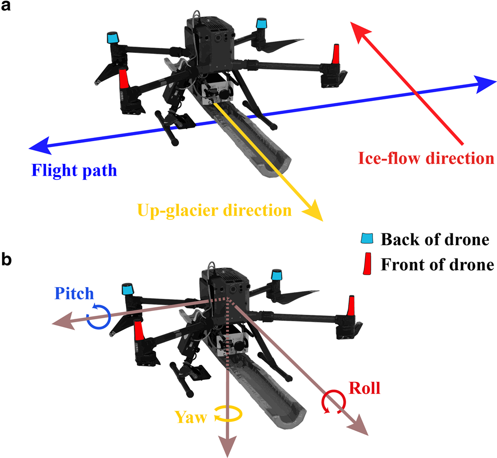
Figure 6. (a) Orientation of the drone-based GPR system during a survey. The front of the drone (red markers) always faces up-glacier, whereas survey lines are flown perpendicular to this direction across the glacier. (b) Illustration of the three flight dynamics parameters.
To evaluate the stability of our system during flight, we now examine the three flight dynamics parameters (yaw, pitch and roll), which are illustrated in Figure 6b. Indeed, even if the drone-based GPR system appears to be visually highly stable during operation, these parameters will vary due to its motion. Figure 7 shows these flight dynamics parameters over ten consecutive profiles from a 3D dataset. The profiles were flown in alternating directions using ABT turns. The programmed drone speed was 4 m s−1. We see that the pitch angle stays close to zero along the profiles, whereas the roll angle alternates from positive to negative values from one profile to another because the antenna position falls slightly behind the drone body during flight. The mean absolute amplitude of the roll angle along the profiles is below 5 degrees, which results in a translation in the location of the GPR antenna of 2.5 cm horizontally and 0.1 cm vertically. These shifts are afterwards corrected when determining the GPS coordinates of the antenna during processing (see Section 4.3). Finally, the yaw angle, relative to the programmed antenna orientation along the flight line, also stays close to zero, further confirming the stability of our system.
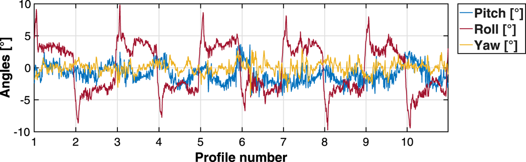
Figure 7. Flight dynamics parameters of the drone-based GPR system over ten consecutive profiles, flown in alternating directions using ABT turns, from a 3D GPR dataset recorded on the Otemma glacier. The programmed drone speed was 4 m s−1. The pitch and roll angles are defined in Figure 6b, whereas the yaw angle is relative to the programmed antenna orientation along the flight line.
4. Example dataset
To highlight the capabilities of our system and the strong potential for drone-based GPR surveying in glaciological studies, we present in this section an example 3D dataset acquired at the Otemma Glacier (Switzerland) in the summer of 2022. Note that our discussion below focuses on the acquisition of the data and on their basic editing and processing in order to obtain a high-quality GPR volume in time. Full details pertaining to depth imaging of the data and their glaciological interpretation are not explored in this paper.
4.1. Field site
The Otemma glacier is a temperate valley glacier located in the Canton of Valais in Southwestern Switzerland (Fig. 8a). It is approximately 7 km long, 600 m wide, and ranges from 2550 to 3790 m elevation. The glacier experienced an average retreat of 32 m per year between 1973 and 2010 (ETHZ VAW, EKK/SCNAT, 2010), and the average ice thickness in 2014 was estimated to be approximately 250 m (Rutishauser and others, Reference Rutishauser, Maurer and Bauder2016). In 2017, a high-density GPR dataset of size ~200 m × 100 m was acquired on foot in the area close to the glacier snout, which allowed mapping of a major and highly sinuous subglacial channel (Egli and others, Reference Egli, Irving and Lane2021a). In the summer of 2018, a large collapse event occurred in the location of the previous GPR survey, which was attributed to the effects of surface ablation combined with melting and block caving inside the channel resulting from the entry of warm air at atmospheric pressure (Egli and others, Reference Egli, Belotti, Ouvry, Irving and Lane2021b). At the time of writing, most of the Otemma glacier is located below the equilibrium line altitude which makes it highly sensitive to increases in average air temperature.

Figure 8. (a) Location of the Otemma glacier (red outline) in southwestern Switzerland (inset). The blue square in the lower ablation zone indicates the region of our GPR survey, which is shown in detail in (b). Profile lines were flown along a southeast-northwest orientation moving up-glacier. Satellite background image in (a) from the Sentinel-2 Mosaic program (NPOC 2020). Inset map in (a) and satellite background image in (b) from the Swiss Federal Office of Topography (Swisstopo).
4.2. Data acquisition
Over the course of four days in August 2022, we recorded a large, high-density, high-resolution, 3D GPR dataset near the Otemma glacier snout with the newly developed drone-based system. To this end, a generator was brought to the glacier so that the drone batteries could be charged directly on-site during acquisition, thereby permitting more profile lines to be surveyed per day than our four sets of batteries would normally allow. The first GPR profile was set to be as close to the glacier snout as possible, and subsequent profiles were surveyed moving up-glacier with a line spacing of 1 m. A grid of 462 parallel profiles of length ranging from 140 to 330 m was surveyed, representing a total of more than 112 line-km of GPR data (Fig. 8b). The approximate area of the grid is 110 000 m2. The drone was programmed to fly at a speed of 4 m s−1 and a height above the glacier surface of 5 m.
4.3. Data editing and processing
Because the GPR trace acquisition rate of our system (14 Hz) differs from the frequency at which GPS data are logged by the GPR controller (5 Hz), interpolation was first performed such that each individual GPR trace could be tagged with precise GPS coordinates. Next, a correction was made to translate these coordinates, which correspond to the location of the RTK antenna, to the location of the center of the GPR antenna (Fig. 1a). To this end, the static offset between the two antennas along with the pitch and roll angles (Fig. 6b) are required. Binning of the GPR data was subsequently performed to create a regular grid of GPR measurements having an inline spacing of 0.4 m and a crossline spacing of 1 m. Thanks to the navigational precision of the drone and thus the limited deviation between the true and programmed coordinates, each GPR profile could be binned independently. This was done by populating each bin with the nearest GPR trace and discarding all other traces, which we have found to provide a cleaner result than averaging over multiple nearby recordings.
Only basic processing of the Otemma 3D GPR dataset was carried out to produce the results presented in this paper. This consisted of the following series of steps, which were performed using customized codes in MATLAB:
i. Time-zero adjustment based on calibration tests of our system to ensure that the zero time on each GPR trace corresponds with the fire time of the transmitter antenna.
ii. Mean trace removal using a sliding 30-trace window to remove the high-amplitude emitted GPR pulse and associated internal antenna and system ringing, which otherwise tend to overshadow many reflected arrivals.
iii. Minor static adjustment of each trace via Fourier phase shift such that the data conform to a smooth acquisition surface, to reduce vertical ‘jumps’ in the data and their corresponding horizontal discontinuities, which are caused by small variations in the height of the drone between survey lines.
iv. Relative adjustment of the position of odd- vs even-numbered profiles based on maximizing the correlation between adjacent flight lines in order to correct for the ‘acquisition pattern’ in the data (Egli and others, Reference Egli, Irving and Lane2021a). Indeed, even though the surveyed positions are measured precisely with dGPS, small internal timing delays combined with the flight speed of the drone mean that such a correction is necessary for optimal results.
v. De-wow using a 13-point residual median filter to remove the low-frequency transient upon which the desired GPR reflections from the glacier are superimposed.
vi. Application of a time-varying gain function based on the average observed decay of GPR amplitudes across the dataset, in order to correct for geometrical spreading losses and the effects of signal attenuation. The smoothed inverse of the average amplitude decay curve curve was utilized.
vii. Fourier-transform-based interpolation in time to quadruple the number of points per trace for improved data display and analysis.
4.4. Results
Figures 9–13 present different views of the Otemma dataset after the editing and elementary processing described above. In Figure 9, we show a 3D view of selected intersecting inline and crossline profiles, which are presented in detail in Figures 10 and 11, respectively. We see on all profiles that the interface between the ice and the bedrock is clearly visible, even down to a two-way travel time of 1000 ns. The latter corresponds to a depth of approximately 80 m assuming a radar speed of 0.167 m ns−1 in glacier ice (e.g. Plewes and Hubbard, Reference Plewes and Hubbard2001) and considering the 5 m layer of air between the antenna and the ice surface. Numerous internal features are also present, as indicated by the various diffraction hyperbolae that can be seen on the sections, most notably in the upper part of the images but also at depth. These features may represent air voids, water pockets, or large boulders in the ice. As an example, the blue ellipses in Figures 9 and 10 highlight the location of a large hyperbola that can be followed over tens of neighboring profiles, which likely represents an air- or water-filled cavity. Tracking the presence of such features in 3D may reveal important and so-far unexplored details about the englacial hydrological system.
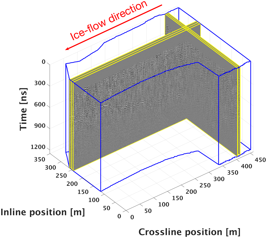
Figure 9. 3D representation of the Otemma GPR dataset as a ‘data cube’, and the location of the three inline and crossline profiles displayed in Figures 10 and 11. The blue outline shows the boundaries of the data volume. The GPR profiles were surveyed perpendicular to the ice flow direction.

Figure 10. Example inline GPR profiles. Three profiles separated by 5 m are depicted. The glacier bed is clearly visible (red arrows), and a large englacial feature can be seen (blue ellipse). The yellow lines denote the intersections with the three crossline profiles shown in Figure 11.


Figure 12. Twelve timeslices from the Otemma 3D GPR dataset taken at regular intervals between 187.5 and 875 ns. The yellow rectangle highlights an elongated englacial feature that is further explored in Figure 13. The red arrows indicate the emergence of the ice-bedrock interface on the northwestern (timeslice at 375 ns) and southeastern (timeslice at 625 ns) sides of the glacier. The blue circles indicate the position of the large englacial feature seen in Figures 10 and 11. The green circle highlights a likely void near the glacier bed.

Figure 13. 3D representation of a sub-volume of the Otemma GPR dataset. A large, elongated feature is visible in the crossline direction, extending 80 m horizontally and 60 ns vertically. The location of this feature is marked by a yellow rectangle in Figure 12.
In Figure 12, we show twelve timeslices through the Otemma 3D dataset, extracted at regular intervals between 187.5 and 875 ns. In the earliest two panels, multiple circles can be observed whose radii grow in time. Such features represent scattered energy from various heterogeneities within the ice and correspond to the various diffraction hyperbolae seen in Figures 9 and 10. At 312.5 ns, and highlighted with a yellow rectangle, we observe the reflection from a major feature which we believe to be another large englacial channel. Figure 13 presents a detailed 3D view of this feature, where we see that it extends over more than 80 m in the crossline direction and over a time range of approximately 60 ns, clearly dipping in the up-glacier direction. Descending further into the dataset in time, we observe, indicated by the red arrows, the emergence of the glacier bed reflection from the northwestern side of the valley near the top of the timeslice at 375 ns, and another large, englacial feature at 437.5 ns and 500 ns, highlighted with a blue circle. The bedrock reflection from the southeastern side of the valley, indicated by a red arrow, can then be seen to emerge near the bottom of the timeslice at 625 ns, followed by another large internal feature at 750 ns, circled in green, which may correspond to a subglacial feature considering its proximity with the bedrock interface.
5. Discussion and conclusions
The research gap that this study aims to fill is the lack of a suitable data acquisition methodology for recording large, high-density and high-resolution 3D and 4D GPR datasets over alpine glaciers in a safe and efficient manner. Recent studies, as well as the field results presented in this paper, suggest that such data have tremendous potential for revealing detailed information about glacier internal structure and bed conditions, which in turn can be used to better our understanding of alpine glacier hydrology and dynamics. To fill this research need, we have developed a drone-based GPR instrument. Construction of this instrument required bringing together (i) a state-of-the-art GPR controller, custom designed for alpine glacier work, having a long recording time and with real-time sampling to permit thousands of stacks while maintaining a high trace output rate; (ii) a lightweight, 80-MHz, GPR transmit–receive antenna; (iii) a terrain-following navigational system; and (iv) a drone equipped with dGPS positioning. This was followed by elaboration of a clear survey methodology to minimize the risk of a crash during the data acquisition, and optimization of a number of flight parameters to find an acceptable balance between data acquisition speed and data quality. It is important to note that, at the time of writing, at least one commercially available drone-based GPR system for geological applications exists (Malå), and it is expected that more will follow. Although our goal here is not to provide a full comparison with the existing system, we should point out that our developed instrument, specifically intended for glacier acquisitions, has approximately half the payload weight of the commercial system and over three times the trace recording length. The former permits longer survey times and compatibility with a wider variety of drones, whereas the latter allows for greater depths of penetration into the ice when possible.
The key limiting factor of our drone-based GPR system for glaciological work is the drone battery consumption. Under realistic field conditions, we can record approximately 4 line-km of high-quality GPR data on a single set of batteries in approximately 20 min. Maximizing the amount of data that can be acquired in a single day therefore means using multiple sets of batteries and/or bringing a generator or power bank on site, such that charging can occur as the survey is ongoing. For the presented 3D acquisition on the Otemma glacier, a combination of four sets of batteries and a fuel generator were used, which allowed us to record a total of 112 line-km of GPR data in only four field days of moderate intensity. The quality of the resulting 3D data volume is high, with a strong reflection coming from the glacier bed at over 80-m depth, and numerous diffraction hyperbolae being trackable over tens of neighboring profiles, likely indicating the presence of englacial channels. Our current work involves detailed exploration of this Otemma dataset in a glaciological context, as well as the development of advanced data migration and interpretation strategies that are beyond the scope of this work. Multiple 4D datasets have also now been collected with the drone-based GPR system and are currently undergoing analysis.
Acknowledgements
We thank Johanna Klahold and Pascal Egli for their help with field testing of the developed GPR system. We also thank Johanna Klahold, Barthélémy Anhorn, Bruno Galissard de Marignac, Edith Sotelo Gamboa, Floreana Miesen, Frédéric Lardet, Jürg Hunziker, Mélissa Francey, Pau Wiersma and the members of the UNIL AlpWISE group for their help with fieldwork on the Otemma glacier. Thanks also to the team at Utsi Electronics Ltd. for their dedicated support in developing the GPR controller, as well as the team at SPH Engineering for their assistance with the True Terrain Following navigation system. Finally, we thank the two anonymous reviewers as well as associate editor Bernd Kulessa and associate chief editor Hester Jiskoot for comments that greatly helped to improve the quality of the manuscript. This work was supported by a grant to J. Irving from the Swiss National Science Foundation (grant number 200021_188575).


 Open access