


Introduction
Sea ice in the Southern Ocean is a driver of the global ocean circulation due to its role in the formation of high-salinity deep water (Gordon, Reference Gordon1988; Ferrari and others, Reference Ferrari2014; Haumann and others, Reference Haumann, Gruber, Münnich, Frenger and Kern2016). Observed trends in sea ice extent around Antarctica have been generally positive since 1979 (Parkinson, Reference Parkinson2019), even though regional differences exist (Stammerjohn and others, Reference Stammerjohn, Martinson, Smith, Yuan and Rind2008). For the period since 2014, however, a decline in sea ice extent has been documented (Parkinson, Reference Parkinson2019). Many driving mechanisms for sea ice variability have been proposed, with studies emphasizing the uncertainty on the exact mechanisms driving variability in Antarctic sea ice extent and volume (e.g. Liu and others, Reference Liu, Curry and Martinson2004; Lefebvre and Goosse, Reference Lefebvre and Goosse2008; Haumann and others, Reference Haumann, Notz and Schmidt2014). Uncertainty on snow cover thickness and distribution has been recognized as a contributing factor to this uncertainty (Hobbs and others, Reference Hobbs2016).
The snow cover on sea ice impacts both the thermal (e.g. Eicken and others, Reference Eicken, Fischer and Lemke1995; Sturm and others, Reference Sturm, Perovich and Holmgren2002; Lecomte and others, Reference Lecomte2013) and the mass balance of sea ice (e.g. Nicolaus and others, Reference Nicolaus, Haas, Bareiss and Willmes2006; Leonard and Maksym, Reference Leonard and Maksym2011). The high albedo of snow reduces the absorption of shortwave radiation, thus reducing incoming energy in the thermal balance (e.g. Curry and others, Reference Curry, Schramm and Ebert1995; Perovich and Polashenski, Reference Perovich and Polashenski2012). In contrast, thermal insulation provided by snow reduces energy loss by the sea ice. The role of snow in the Arctic sea ice thermal balance is particularly via albedo (Nicolaus and others, Reference Nicolaus, Haas, Bareiss and Willmes2006), which can fluctuate from low albedo for melting snow to high albedo for fresh snow on short time scales (Perovich and others, Reference Perovich, Polashenski, Arntsen and Stwertka2017). Southern Ocean sea ice generally has thicker snow covers and thinner ice conditions than exist in the Arctic, so the insulation effect dominates over the albedo effect (Massom and others, Reference Massom2001; Nicolaus and others, Reference Nicolaus, Haas, Bareiss and Willmes2006; Maksym, Reference Maksym2019). In addition to the insulation properties of snow, thick snow covers on thin ice may lead to widespread flooding and snow–ice formation in the Southern Ocean (Maksym and Markus, Reference Maksym and Markus2008). Flooding is defined here as the entering of sea water and/or brine in the snow cover, either via cracks in the ice or via brine channels. Flooding creates a slushy layer at the bottom of the snow cover, which, upon refreezing, forms a layer referred to as snow ice. Snow–ice formation provides a positive impact on the sea-ice mass balance (Powell and others, Reference Powell DC, Markus T and Stössel A2005).
Remote-sensing and in situ observations have shown that the snow cover and ice thickness of sea ice in the Southern Ocean vary within large ocean basins. For example, sea ice is generally thicker than 1 m in the western Weddell Sea in all seasons, whereas it is thinner than 1 m in the eastern Weddell Sea, even in spring (e.g. Kurtz and Markus, Reference Kurtz and Markus2012). Similarly, snow depth is variable across the Southern Ocean, with a maximum towards the western Weddell Sea and elsewhere along the coast where ice survives into the summer (Worby and others, Reference Worby, Markus, Steer, Lytle and Massom2008). The correspondence between areas with thick ice and deep snow covers is not a coincidence: this spatial variability is partly driven by ice age (and thus accumulation time), but also sea ice roughness providing sheltered spots where wind-transported snow can accumulate (Markus and others, Reference Markus2011). Furthermore, spatial variability in snow cover thickness also impacts snow properties, such as grain size and grain type (Arndt and Paul, Reference Arndt and Paul2018), since the temperature gradients controlling snow metamorphism processes decrease with increasing snow thickness (Sommerfeld and LaChapelle, Reference Sommerfeld and LaChapelle1970; Arndt and Paul, Reference Arndt and Paul2018). In turn, the microstructure determines properties of the snow cover with an impact on the thermal balance of the sea ice, such as surface albedo (e.g. Aoki and others, Reference Aoki, Hachikubo and Hori2003) and thermal conductivity (e.g. Riche and Schneebeli, Reference Riche and Schneebeli2013).
The snow and ice thickness also exhibits strong spatial variability on the floe-scale. Snow redistribution by the wind causes dunes even in the absence of ridged ice (Sommer and others, Reference Sommer, Wever, Fierz and Lehning2018; Moon and others, Reference Moon2019). Due to ridging and rafting, the sea-ice thickness can vary considerably on sub-kilometer scale (Williams and others, Reference Williams2015). The presence of underlying variability in ice thickness in turn increases variability in the snow-depth distribution (Trujillo and others, Reference Trujillo, Leonard, Maksym and Lehning2016; Liston and others, Reference Liston2018). Note that snow preferentially accumulating near pressure ridges (Massom and others, Reference Massom, Drinkwater and Haas1997; Déry and Tremblay, Reference Déry and Tremblay2004; Liston and others, Reference Liston2018) effectively decreases the spatial variability (i.e. smooths) of the surface (Adolphs, Reference Adolphs1999).
Given the large-scale spatial variability in snow and ice thickness, combined with spatially-varying snowfall, flooding and snow–ice formation is also spatially variable (Jeffries and others, Reference Jeffries, Roy Krouse, Hurst-Cushing and Maksym2001; Maksym and Markus, Reference Maksym and Markus2008). Those authors found snow-ice formation to be widespread in level ice, with an average thickness of 16 cm in September compared to an average ice thickness of 70 cm. For the Weddell Sea, ~10–15 cm of snow–ice formation was found, whereas in areas near the coast of East Antarctica, in the Amundsen Sea and the outer Ross Sea, up to 30 cm of snow–ice formation may occur, with snow ice then making up 12–36% of total ice mass. The impact of ridged ice, where thickness can vary largely over scales of a few meters, is more difficult to assess.
To measure snow and ice thickness in situ, ice mass-balance buoys (IMBs) and snow buoys are commonly used (Jackson and others, Reference Jackson2013; Grosfeld and others, Reference Grosfeld2015). These devices are typically point measurements, and even though it is tempting to interpret the data as being representative for the floe-scale spatial variability, this requires careful site selection (Perovich and Richter-Menge, Reference Perovich and Richter-Menge2006; Polashenski and others, Reference Polashenski, Perovich, Richter-Menge and Elder2011). At the same time, remote sensing methods generally capture only large-scale spatial variability because footprints exceed the typical length scales of the meter-scale variability (Kwok, Reference Kwok2010; Kwok and others, Reference Kwok2011; Lawrence and others, Reference Lawrence, Tsamados, Stroeve, Armitage and Ridout2018; Li and others, Reference Li2018; Rösel and others, Reference Rösel2018). Airborne observations can resolve the meter-scale variability, albeit with lower spatial and temporal coverage (Kurtz and others, Reference Kurtz2013), while satellite-based remote sensing still continuously improves (Markus and others, Reference Markus2017).
Similar to in situ observations, many sea-ice models are one-dimensional (1-D) (e.g. Bitz and Lipscomb, Reference Bitz and Lipscomb1999; Maksym and Jeffries, Reference Maksym and Jeffries2000; Nicolaus and others, Reference Nicolaus, Haas, Bareiss and Willmes2006; Griewank and Notz, Reference Griewank and Notz2013; Wever and others, Reference Wever2020), anticipating that point simulations are representative for larger scales. Other models are designed to explicitly capture large-scale variability (Petty and others, Reference Petty, Webster, Boisvert and Markus2018; Hunke and others, Reference Hunke2019), even though they rarely address the floe-scale variability explicitly. The floe-scale variability in snow and ice thickness is typically only described based on the relative presence of thickness classes within a grid point.
Here, we present a high-resolution dataset of floe-scale variability in snow and ice thickness observed during a field campaign in the Weddell Sea, Antarctica during austral winter 2013. These datasets are used to drive spatially distributed simulations that capture the small-scale spatial variability on the floe-scale. The simulations are compared to 1-D simulations for floe-averaged snow and ice thickness, as well as 1-D simulations of the IMB conditions, to investigate the correspondence between point and distributed simulations.
Data
The Antarctic Winter Ecosystem and Climate Study (AWECS, ANT-XXIX/6) onboard R/V Polarstern surveyed the Weddell Sea between June and August 2013 (Lemke, Reference Lemke2014). During several ice stations, some of which were 12 h while others lasted for 4–5 d, field work was carried out on sea-ice floes. We collected observations of snow and ice thickness using Terrestrial Laser Scanning (TLS), Magnaprobe, and the multi-frequency electromagnetic induction instrument GEM-2. At one ice station, the snow density was surveyed with a SnowMicroPen (SMP). Here we describe data from three ice stations: PS81/503, PS81/506 and PS81/517 (see Table I). For those ice stations, data acquisition from TLS were of good quality (no drifting snow and accurate registration), and the Magnaprobe and GEM-2 survey was completed. PS81/503 and PS81/506 were first-year floes, and PS81/517 was a multi-year floe (Arndt and Paul, Reference Arndt and Paul2018). Simulations are only performed for two of these ice stations, where IMBs were installed that remained operational for longer than a month after deployment. Figure 1 shows the location of the three ice stations.

Fig. 1. The three ice stations (labeled PS81/5XX) and trajectories of the two IMBs used in this study, for (a, b) ice thickness and (c, d) snow depth, as determined from the IMB data. When the trajectory is colored gray, ice and/or snow thickness could not be determined due to poor data quality. The installation location of each IMB coincides with the location of an ice station (circles), the last reported location by each IMB is shown by the squares. The position of the 1st and 15th days of each month is labeled.
Table 1. Ice station coordinates, start date, duration and collected measurements and installed buoys

a As reported by Arndt and Paul (Reference Arndt and Paul2018).
Figures 2 and 3 show the maps of the measurement layout for both ice stations PS81/506 and PS81/517, respectively, and Figure S1 in Supplementary material shows the map for ice station PS81/503. Figures S2–S4 in Supplementary material show the details of the maps for the TLS field for the three ice stations, respectively.
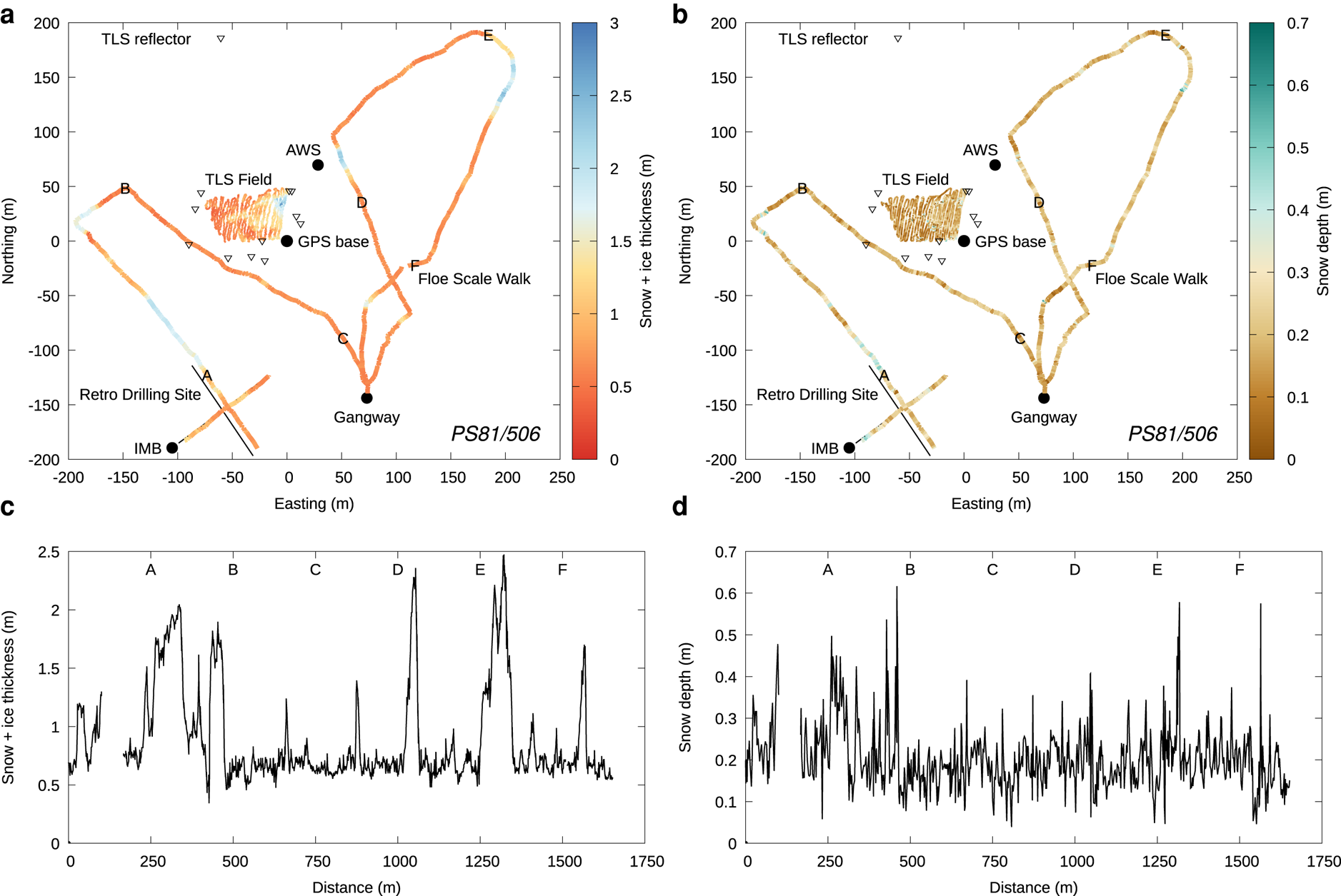
Fig. 2. Map of ice station PS81/506 in a floe-based coordinate system, with northing and easting aligned with WGS 84/UTM zone 27S (EPSG 32727) at the start of the Magnaprobe survey, with colors denoting (a) snow+ice thickness from GEM-2, and (b) snow depth from Magnaprobe. The black dots denote the GPS surveyed points, the triangles denote the TLS reflectors and the black lines denote the retro-drilling transects. Lower panels show snow+ice thickness (c) and snow depth (d) along the floe-scale walk, with markers A to F showing corresponding points between the graphs and the maps in (a, b).

Fig. 3. Map of ice station PS81/517 in a floe-based coordinate system, with northing and easting aligned with WGS 84/UTM zone 22S (EPSG 32722) at the start of the Magnaprobe survey, with colors denoting (a) snow+ice thickness from GEM-2, and (b) snow depth from Magnaprobe. The black dots denote the GPS surveyed points, the triangles denote the TLS reflectors and the black lines denote the retro-drilling transects. The blue lines in the TLS field denote the SMP transects. Blue labels starting with ‘SP’ denote the location of the eight snow pits used to calibrate the SMP. Lower panels show snow + ice thickness (c) and snow depth (d) along the floe-scale walk, with markers A to F showing corresponding points between the graphs and the maps in (a, b).
On each floe, two GPS base stations were temporarily installed, measuring continuously for the duration of the ice station, whereas a third GPS was used for conducting the surveys. This enabled the use of post-processing kinematic GPS (PPK-GPS), providing a coordinate system relative to one of the GPS base stations, in a coordinate system that is invariant under floe drift and rotation. The start of the Magnaprobe surveying was considered the synchronization point and all floe drift and rotation before and after that has been corrected for.
During each ice station, an automatic weather station (AWS) buoy and an IMB were permanently installed on the floe to monitor the temporal evolution of the ice and weather conditions. Only two IMB/AWS pairs survived for a useful period for analysis with sufficient data quality to be included in this study.
Terrestrial laser scanning
At each ice station, a visually seemingly representative patch of snow was selected. On 4–5-day ice stations, the surface topography of a patch of ~50 × 50 m was surveyed from multiple locations at the edge of the patch, with a Riegl LPM-321 terrestrial laser scanner. The scanner uses a near-infrared (905 nm) laser (Prokop and others, Reference Prokop, Schirmer, Rub, Lehning and Stocker2008; Grünewald and others, Reference Grünewald, Schirmer, Mott and Lehning2010). On the 10-h ice station, a FARO Focus3D-S 120 scanner was used, which measures using phase shift of an infrared laser.
For referencing the scans, around ten reflectors were installed on plastic pipes. Each reflector was surveyed with PPK-GPS to locate them inside the floe-based coordinate system. The measured freeboard and reflector height above the snow surface at the reflector locations was used to correct the elevations from GPS-defined elevation to the actual sea level. By drilling completely through the ice when installing the reflectors, the precise height of each of the reflectors above sea level could be directly measured. The reflectors were used to combine multiple scan positions into one coherent point cloud and to reference the vertical coordinate of the combined point cloud to sea level. Registering the multiple scan positions was possible with a standard deviation of the reflector coordinates in the order of 3–5 cm. This error determines the error in the scanned surfaces and includes errors due to instabilities in the laser scanner tripod, GPS related errors in determining reflector positions as well as instabilities in the reflector setup. The vertical error in GPS-surveyed elevation for each reflector, which combines the error in sea level measurements and the accuracy from GPS is 5 cm. Since we used up to ten reflectors, the error in elevation after registration is estimated to be considerably smaller.
Magnaprobe
After all TLS scans were acquired, the laser scanning area was surveyed by a Magnaprobe (Snow Hydro, Fairbanks, AK, USA) to measure point snow depths above the ice surface (Sturm and Holmgren, Reference Sturm and Holmgren2018). The Magnaprobe was combined with a PPK capable GPS receiver, such that every individual snow measurement can be located accurately inside the floe-based coordinate system. The maximum measurement depth of the device is 1.2 m. The probe is designed to penetrate the hard wind-packed snow (Sturm and Holmgren, Reference Sturm and Holmgren2018), and the observer generally felt a hard transition to the ice surface. Additionally, a Magnaprobe measurement series was acquired by walking around the floe, which we will refer to as the floe-scale walk (see Fig. S1b in Supplementary material and Figs 2b, 3b). In both cases, the measurement spacing is about 1–2 m. The point snow thicknesses acquired by the Magnaprobe can be combined with the TLS surface to determine ice-freeboard and snow depth (Williams and others, Reference Williams2013; Trujillo and others, Reference Trujillo, Leonard, Maksym and Lehning2016).
GEM-2
By directly following the Magnaprobe surveyor, the floe was also surveyed by a ground-based, multifrequency electromagnetic induction instrument (GEM-2, Geophex Ltd.) (Hunkeler and others, Reference Hunkeler, Hendricks, Hoppmann, Paul and Gerdes2015, Reference Hunkeler2016). The GEM-2 detects the sea ice–ocean interface, which then provides the total snow and ice thickness below the instrument. Measurements were acquired at 10 Hz and the accuracy for level ice up to 3 m thick is 0.1 m (Hunkeler and others, Reference Hunkeler, Hendricks, Hoppmann, Paul and Gerdes2015). Datasets of total snow and ice thickness for both the TLS field, as well as for the floe-scale walk were acquired (see Fig. S1a in Supplementary material and Figs 2a, 3a). For the floe-scale walk, no calibration of the GEM-2-based GPS took place, so the coordinates have been matched here using the time stamp. This results in a typical location error of 2–5 m, corresponding to the distance between the Magnaprobe and GEM-2 instrument during the surveying.
Retro-drilling
During each ice station, snow depth, ice thickness and freeboard were determined using a 5 cm auger (Kovacs Enterprise) and a sea-ice thickness measurement gauge for ice thickness and a wooden ruler for snow thickness. As in Lemke (Reference Lemke2014), we refer to this as retro-drilling to contrast the classical, direct way of measuring ice thickness with more recently developed indirect methods. Two more or less perpendicular transects of 100 m length in a cross-shaped were sampled at 5 m intervals (see Fig. S1 in Supplementary material and Figs 2, 3).
SnowMicroPen
We used a SMP, version 3, to survey the snow properties in the uppermost 25–30 cm of the snowpack at ice station PS81/517. The variability in measurement depth is determined by the varying distance between the instrument and the snow surface, when positioning the instrument on an uneven snow surface.
The SMP measures the penetration resistance for a constant penetration speed, using a very sensitive force sensor (Johnson and Schneebeli, Reference Johnson and Schneebeli1999). The median force ($\widetilde {F}$ , N) was related to the snow density (ρ, kg m−3) using (Löwe and van Herwijnen, Reference Löwe and van Herwijnen2012; Proksch and others, Reference Proksch, Löwe and Schneebeli2015):

We calibrated the SMP instrument using eight collocated snow pits (Paul and others, Reference Paul, Arndt and Stoll2017; Arndt and Paul, Reference Arndt and Paul2018) and SMP measurements (see Fig. 3) to fit coefficients a 1 and a 2 with the following procedure. For each snow pit, three to four SMPs were acquired within 10–30 cm distance from the snow pits. For the calibration, the median force was determined over the same 3 cm thick layers as reported for the snow pits. A vertical offset was applied to the SMP profiles ranging from +3 to −3 cm, in steps of 0.01 cm, to account for locally varying snow depths. For each SMP, the offset that provided the highest correlation between the density from the manual density cutter and the natural logarithm of the median force from the SMP was determined. Then, the SMP with the highest correlation was considered representative for the snow pit, and was used to calibrate the SMP with the snow pit.
After calibration, the average snow density in both snow pits and SMP measurements is 269 kg m−3. The standard deviation in the density from the snow pit measurements (54 kg m−3) is larger than from the SMP measurements (31 kg m−3). The correlation coefficient after calibration is 0.58 (p < 0.001). The comparison between snow pits and SMP measurements is shown in Supplementary material, Figure S5.
For PS81/517, two transects were made inside the TLS field (see Fig. 3) using the SMP. The transects were located inside the TLS field by combining the instrument's own GPS and measured distances with other known GPS-surveyed objects. SMPs were taken with a spacing of ~30 cm. The general positioning accuracy of the SMPs inside the coordinate system is estimated to be smaller than 1–2 m. For each SMP in these transects, the snow surface above sea level was determined by taking the average surface height of all TLS points inside a 15 cm radius around the SMP measurement.
Ice-mass balance buoys
At two ice floes, IMBs provided by the Scottish Association for Marine Science (SAMS) were installed to collect continuous measurements of sea ice temperatures. The IMBs consist of a temperature sensor string of 5 m, with a sensor spacing of 2 cm (Jackson and others, Reference Jackson2013). Furthermore, the sensor chain was heated once a day to use the temperature response along the string as an indicator whether the surrounding media was ocean, sea ice or snow, based on differences in thermal response. From the temperature and heating rate measurements, the interfaces (ocean–sea ice, sea ice–snow and snow–atmosphere) were manually determined. The ice–ocean interface was identified by the knee in the vertical temperature profile when a gradient existed in the ice, assisted by differences in the heating rate profile (for WHOI$\_$ 05 at PS81/506). The snow–air interface was similarly identified, but also by examining the diurnal variability in the temperature profile, as air temperatures can change more rapidly than snow temperatures. Flooding was clearly visible via changes in the heating rate profile over time at the base of the snow layer. The flooded snow layers show a strong reduction in heating rate due to the high heat capacity of the liquid water in those layers. The estimated accuracy of these interface determinations is 2–4 cm. Each IMB was equipped with a GPS receiver to track the floe drift.
Meteorological data
At PS81/506 and PS81/517, automated weather station buoys were installed on the sea ice. Two Wenglor YH08NCT8 sensors (Wenglor Corporation) per buoy were used as snow particle counters (SPCs) to measure drifting snow particles (Leonard and others, Reference Leonard, Tremblay, Thom and MacAyeal2012). One SPC was installed close to the snow surface (44 cm and 31 cm for PS81/506 and PS81/517, respectively), to particularly capture drifting snow, while the second SPC was installed at 183 and 179 cm, respectively, to capture precipitation. Air temperature and relative humidity were measured at 1.85 m (PS81/506) and 1.82 m (PS81/517), and wind speed and direction were measured at 2.50 ± 0.03 m (PS81/506) and 2.27 ± 0.03 m (PS81/517), respectively.
The last received data from the AWS installed at ice station PS81/517 were from 12 November 2013, 12:00 UTC and showed the battery level dropping well below operating level, indicating that this was the likely cause of failure of the AWS. For PS81/506, the AWS showed healthy battery levels upon the last transmission on 15 August 2013, 13:59:59 UTC and it is unclear why data transmission was lost.
Since not all variables needed to run the simulations are measured by the AWS, and the AWS installed at PS81/506 measured for only a brief period, we force the simulations with data from the Modern-Era Retrospective analysis for Research and Applications, Version 2 (MERRA-2) (Gelaro and others, Reference Gelaro2017). The MERRA-2 model was found to adequately represent precipitation in the Weddell Sea area, compared to other reanalysis products (Boisvert and others, Reference Boisvert2020). For each hourly MERRA-2 time step, the closest model grid point to the location of the IMB was taken to extract the required forcing variables (near-surface air temperature, relative humidity, wind speed, incoming shortwave and longwave radiation, and precipitation).
Methods
SNOWPACK model and Alpine3D model
The SNOWPACK model (Bartelt and Lehning, Reference Bartelt and Lehning2002; Lehning and others, Reference Lehning, Bartelt, Brown, Fierz and Satyawali2002a, Reference Lehning, Bartelt, Brown and Fierz2002b), has been recently adapted for sea ice (Wever and others, Reference Wever2020). The model has a detailed snow microstructure description, and solves heat flow and phase changes. The model enforces thermal equilibrium between brine and solid ice, while taking into account the freezing point depression due to the presence of salt.
We use the Richards equation (Wever and others, Reference Wever, Fierz, Mitterer, Hirashima and Lehning2014), combined with the transport equation for salinity to solve liquid water and brine distributions (Wever and others, Reference Wever2020). This approach simulates liquid water flow based on pressure head distributions for both the saturated part (Darcy flow), as well as unsaturated flow which mostly occurs in the snowpack. Salinity changes are simulated by advection based on the liquid water flow calculated by the Richards equation and diffusion. The internal flow is governed by the positive pressure head at the bottom of the sea ice corresponding to the displaced water.
The water flow in the snow-sea ice system is governed by porosity, which can vary from as high as 95% for new snow under low wind speed conditions to the lower limit set for sea ice of 1%. Note that the lower limit is required for numerical stability (Wever and others, Reference Wever2020). The porosity varies over the course of a simulation due to snow settling, snowmelt or melting or freezing of brine. The porosity in turn poses a strong control on hydraulic conductivity. In SNOWPACK, the hydraulic conductivity is parameterized by combining a parameterization for snow (Calonne and others, Reference Calonne2012), with one for sea ice (Golden and others, Reference Golden2007), depending on porosity (Wever and others, Reference Wever2020).
In Wever and others (Reference Wever2020), it was noted that new snow density may be underestimated for polar regions with default settings for the SNOWPACK model, which typically describe alpine conditions. Underestimating new snow density leads to an overall underestimation of snow density. We modified the model such that modifications for polar regions to improve the simulated snow density, as presented in Steger and others (Reference Steger2017), are now also available for sea ice simulations. This entails an enhanced compaction of snow under the influence of wind, as noted by Brun and others (Reference Brun, Martin and Spiridonov1997), and implemented in SNOWPACK according to Groot Zwaaftink and others (Reference Groot Zwaaftink2013). Other modifications describe a fine-grained snow microstructure of snow deposited in drifting snow conditions.
We perform two 1-D simulations for each floe: one with the snow and ice thicknesses as measured upon installation of the IMBs, and one with average snow and ice thickness inside the TLS field. Additionally, we perform spatially distributed simulations to assess the mass balance of the floe as a whole exploiting the spatial fields of snow depth and snow and ice thickness acquired inside the TLS field. The SNOWPACK model can easily be used in a distributed way by employing the Alpine3D overarching model framework (Lehning and others, Reference Lehning2006). The Alpine3D model can run a SNOWPACK simulation for each grid point in parallel for computational efficiency.
Each surface grid point in Alpine3D is independent of neighboring grid cells. Lateral flow of heat and water is ignored. Snow transport by wind is an important process that can spatially redistribute snow on sea ice. It causes snow to typically accumulate unevenly over Antarctic sea ice (e.g. Trujillo and others, Reference Trujillo, Leonard, Maksym and Lehning2016), and particularly behind pressure ridges and other obstacles (Massom and others, Reference Massom, Drinkwater and Haas1997; Liston and others, Reference Liston2018). Here, we employ the Winstral and others (Reference Winstral, Elder and Davis2002) algorithm, which is built into the MeteoIO preprocessing library (Bavay and Egger, Reference Bavay and Egger2014) used by Alpine3D and SNOWPACK.
The original Winstral algorithm is based on terrain analysis to identify wind-sheltered and wind-exposed areas based on the current wind direction. Wind-exposed pixels are provided with a reduced precipitation amount on the current time step and vice versa. We provide a field of elevation above sea level to the algorithm, which is updated each hourly time step, such that the elevation changes are taken into account for determining wind-sheltered and wind-exposed areas. As we lack information about floe rotation, we simply apply a linear increase of 2.14° h−1 in the wind direction, corresponding to a period of 1 week. We lack repeat laser scans as the buoys drifted to validate the wind redistribution algorithm, but the most important goal is that snow preferentially accumulates in sheltered, low-elevation areas.
We found no noticeable difference in the simulated amount of flooding whether or not the Winstral-algorithm was used. Therefore, we will not discuss this in more detail. Since we do not consider floe bending, which may be a valid assumption for short length scales but not over tens to hundreds of meters, the hydraulic balance we calculate is not impacted by the exact location of snow accumulation. It is also important to note here that our field datasets of snow depth variability explicitly capture spatial variability of the initial snow depth. Since we assume the ice topography to remain constant and do not consider new pressure ridges forming, the majority of adjustment of the snow cover over the pressure ridges could already be present in our initialization fields. Furthermore, field data support the notion that spatial distribution of snow on the sea ice can be relatively constant, when the underlying ice topography does not change (e.g. Trujillo and others, Reference Trujillo, Leonard, Maksym and Lehning2016).
Floe buoyancy
It is necessary to apply the effect of mass changes due to snowfall, flooding and basal ice growth/melt on the buoyancy of the ice floe, as the grid cells should be connected and individual grid cells are not supposed to move in the vertical direction relative to one another. Flexure of sea-ice floes due to either ocean swell or snow load (Petrich and Eicken, Reference Petrich and Eicken2016) is not considered here.
We now describe how Alpine3D treats the buoyancy of the sea-ice floe. First, each grid cell is internally referenced to sea level. This reference level is defined as the vertical distance between the sea level and the first element (bottom element of the sea ice at the ice/ocean interface) for each grid cell. In turn, the internal sea level provides the bottom boundary condition in terms of pressure head for the Richards equation (Wever and others, Reference Wever2020) to solve the flow of brine and fresh water in the snow/sea ice system. For example, when the additional load from snow fall pushes the sea ice deeper into the water, the pressure head at the bottom increases. Subsequently, hydraulic conductivity in the sea ice, which is a function of brine volume, determines the influx rate of ocean water at the bottom of the sea ice.
The approach detailed in Wever and others (Reference Wever2020) needs to be refined for this study. Each individual grid point in Alpine3D may vary in basal sea ice growth or melt, accumulation, and amount of flooding, but the impact on the bottom pressure head following these changes depend on the behavior of the floe as a whole, and not only on the hydrostatic balance of an individual grid point. The distributed simulations treat the hydrostatic balance with a two-step algorithm. In the first step, bottom ice growth or melt will initially respectively increase or decrease the variable tracking the sea level inside the model domain, such that the same model layer remains associated with the sea level. The buoyancy remains unaltered in this step.
After each hourly time step t, the total mass (T t, kg m−2) of the simulated ice floe is calculated, which then includes mass changes from snowfall, basal ice growth or melt, and brine flux at the bottom of the sea ice (which includes flooding):

where n sums over all N grid cells and m sums over all the M layers in grid cell n. θi,m and θw,m are the volumetric content of ice and water (m3 m−3), respectively, in layer m with layer depth h m (m). The density of ice (ρi) is constant (917 kg m−3), while the density of brine in a layer (ρw) is a function of brine salinity (Wever and others, Reference Wever2020). The bulk density is thereby a function of ice and water content (brine), and the density of brine.
From the total mass T, the average sea level in the model domain, which would obey hydrostatic balance, ($\overline {H_{{\rm sl}}}$ ) can be calculated as:

where ρo is the density of ocean water, where in this study, ocean salinity is set to 35 g kg−1. The sea level change over a time step Δt, ΔH sl, is then given by:

which is then applied to the sea level at the individual grid points.
We set initial sea level in the model domain based on the field measurements of freeboard. Recall here that the TLS topographic survey was referenced to sea level by using the measurements of sea level observed in holes drilled to install the TLS reflectors. Combining this with the TLS and GEM2 data provides the distance from the bottom of the sea ice to sea level for each individual grid point. This setup is congruent with field observations, in which it was found that the hydrostatic balance may hold on the floe scale, but not for point measurements (Forsström and others, Reference Forsström, Gerland and Pedersen2011).
Another option is to initialize the floe in hydrostatic balance. However, in this case, we encountered stability issues in the distributed simulations when the enforced sea level exceeded the total snow and ice thickness. This leads to a positive pressure head at the top of the domain, which the numerical scheme cannot handle.
Initial fields
The model is initialized with a three-dimensional (3-D) description of each floe we visited, by combining the observations of surface topography, snow thickness and total (snow+ice) thickness.
First, data were aggregated into a regular grid, with 10 cm grid cell spacing, using inverse distance weighting to a power with nearest neighbor searching using the tool gdal_grid, part of the gdal-library (GDAL Development Team, Reference GDAL Development Team2016). The following settings were used: a smoothing factor of 0.05, an exponent of 1.0, a radius of 3.0 m, minimum points 3 and maximum points 6. For the GEM-2 data, data were filtered before aggregation, because the measurement frequency of 10 Hz gives much denser coverage of data points along the followed path compared to the distance between paths. Furthermore, the footprint of the device is assumed to extend over the device size. Therefore, we only kept data points from the GEM-2 that were further than 50 cm apart.
Using the tool gdal_translate, the grids were downscaled to 1 × 1 m2 grids, which were used by the Alpine3D simulations. Figures 4a, b show the initial maps of snow and snow+ice thickness, respectively, as used by the simulations, for PS81/506. Similarly, Figures 5a, b show the initial fields for PS81/517.

Fig. 4. Maps of snow thickness (a, d, g), snow+ice thickness (b, e, h) and flooded layer depth (c, f, i) from the distributed simulation for ice station PS81/506 for initial conditions on 15 July (a, b, c), around half-way into the simulation on 1 November (d, e, f) and towards the end of the simulation on 1 February (g, h, i).

Fig. 5. Maps of snow thickness (a, d, g), snow+ice thickness (b, e, h) and flooded layer depth (c, f, i) from the distributed simulation for ice station PS81/517 for initial conditions on 1 August (a, b, c), around half-way into the simulation on 1 September (d, e, f) and towards the end of the simulation on 14 October (g, h, i).
For both Alpine3D and stand-alone SNOWPACK simulations, snow layers were initialized with a density of 275 kg m−3, corresponding to a volumetric ice content of 0.3 m3 m−3 with the remaining part assigned to the volumetric air content (0.7 m3 m−3). Arndt and Paul (Reference Arndt and Paul2018) report a density ranging from 258 to 281 kg m−3 for measurements on the same sea-ice floes. The grain microstructure was set to a grain radius of 0.15 mm, a bond radius of 0.09 and sphericity and dendricity of 0. Temperatures measured by the installed IMBs were used to initialize the vertical temperature profiles, after the temperature fluctuations stabilized, indicating refreezing of the hole drilled for the installation of the thermistor string. The temperature profile was scaled to match ice and snow thickness at the pixel location. For layers a.s.l., the ice layers were initialized with a volumetric ice content of 0.95 m3 m−3 and the remaining 0.05 m3 m−3 was considered air-filled pore space, whereas layers below sea level, where assigned water and a bulk salinity of 1.75 g kg−1, with a volumetric ice and water contents assuming thermal equilibrium. This resulted in a brine volume of around 3–5%. Note that this approach was motivated by earlier work (Wever and others, Reference Wever2020), but that values for the brine volume are lower than observed in the field (mostly ranging between 5 and 12%) during the same measurement campaign by other groups at other parts of the floe (Tison and others, Reference Tison2017). The effect of initial conditions on the results will be discussed later.
Note that several grid points exhibited deeper snowpacks than the surface elevation a.s.l. (i.e. a negative freeboard, and susceptibility to flooding). For the simulation of PS81/506, this was the case for 36 out of 2980 grid points used in the simulation, while for PS81/517, 1163 out of 2819 showed a sea level inside the snowpack. In those cases, the sea level was positioned 2 cm below the snow–ice interface for numerical stability upon initialization. Figures 4c and 5c illustrate that the simulations were initialized without flooding conditions anywhere in the domain. Note that for PS81/517, the negative freeboard was 0–2 cm inside the snowpack for 495 of the 1163 grid points with negative freeboard derived from the observations.
Model setup
The top boundary condition for the heat equation is prescribed as a Neumann boundary condition, with a heat flux resulting from the net surface energy balance. This is calculated using a roughness length of 0.007 m, and an atmospheric stability correction following Michlmayr and others (Reference Michlmayr2008) for calculating turbulent heat fluxes.
At the lower boundary, an ocean heat flux needs to be specified. Values reported for ocean heat flux in the Weddell Sea vary widely, ranging from as low as 2–7 W m−2 in the western Weddell Sea (Robertson and others, Reference Robertson, Padman and Levine1995; Lytle and Ackley, Reference Lytle and Ackley1996) to well over 20 W m−2 in observations in the central Weddell Sea (McPhee and others, Reference McPhee, Kottmeier and Morison1999). We set the ocean heat flux to 8 W m−2 for the simulations shown here, unless noted otherwise.
For the salt transport equation describing the salinity evolution inside the domain, there are separate boundary conditions for the advection and diffusion terms. For advection terms, incoming water flux at the bottom of the domain has an ocean water salinity, incoming water flux at the top of the domain consists of fresh water (rain, condensation). A zero-flux boundary condition is applied at the top of the domain for outgoing water fluxes, such that salt is retained in the sea ice upon evaporation. Similarly, no diffusive exchange of salt with the atmosphere is allowed. Outgoing water flux at the bottom of the domain entails a Neumann boundary condition for the transport equation for salinity. Also the diffusion of salt with the underlying ocean is allowed. These settings are equal to the ones used in Wever and others (Reference Wever2020).
Results and discussion
Snow and ice thickness distributions
Multiple sources of information on snow and ice thickness are available for the visited floes. This section provides a description of the floes visited and demonstrates to what extent the various observations are consistent. Furthermore, since we initialize the simulations with the snow and ice thickness distributions obtained inside the TLS field, we also analyze how representative these measurements are relative to the floe scale.
In Figures 6 and 7, we compare snow and ice thickness distributions derived for the TLS field with the distributions acquired on the floe-scale walk, the direct measurements from the retro-drilling survey, and the snow and ice thickness observed upon installation of the AWS buoy and IMB, respectively, for ice stations PS81/506 and PS81/517. Figure S6 in Supplementary material shows a similar plot for ice station PS81/503.

Fig. 6. Snow thickness, freeboard and snow+ice thickness distributions for ice station PS81/506, based on floe-scale Magnaprobe and GEM-2, Magnaprobe and GEM-2 inside the TLS field, the retro-drilling survey, and measurements upon installation of the AWS buoy and IMB. Distributions are shown as the violin plots (Hintze and Nelson, Reference Hintze and Nelson1998). The violin plot combines a box plot (shown in black, indicating the median by a white dot, the interquartile range by a black box and either the minimum or maximum value or 1.5 times the interquartile range, whichever is closer to the median, by the black lines) with a symmetrically plotted rotated kernel density which shows the full, smoothed and distribution.

Fig. 7. As Figure 6, but for ice station PS81/517. Due to thick ice, ice thickness and freeboard were not determined upon installation of the AWS.
For ice station PS81/506 on first-year ice (Fig. 6), we find a good correspondence in the median value and the standard deviation for the snow depth determined by the Magnaprobe inside the TLS field (0.15 ± 0.10 m) and on the floe-scale walk (0.19 ± 0.08 m). The retro-drilling exhibits slightly higher snow depth (0.24 ± 0.09 m). The total snow and ice thickness as surveyed using GEM-2 shows a good correspondence between the TLS field (0.93 ± 0.45 m) and the retro-drilling survey (0.89 ± 0.43 m), whereas the floe-scale walk survey shows a lower total thickness (0.68 ± 0.45 m).
At the locations where the AWS buoy and IMB were installed, snow depth (0.18 and 0.13 m, respectively) and total thickness (0.84 and 0.88 m, respectively) correspond well with the median values observed inside the TLS field. We therefore assume that the data acquired inside the TLS field is representative for the location of the IMB, even though the buoy was installed about 250 m away from the TLS field. Freeboard with respect to the snow–ice interface at the AWS buoy and IMB locations was found to be positive (0.08 and 0.04 m, respectively). Interestingly, the retro-drilling surveys show an occasional negative freeboard, with a median freeboard of 0 m. This suggests that the specific area was close to being susceptible to flooding.
Ice station PS81/517 on multi-year ice (Fig. 7) generally had thicker ice and greater snow depths than PS81/506 (Fig. 6). The median and the standard deviation of snow depth from the Magnaprobe survey for the floe-scale walk and the TLS field are 0.59 ± 0.24 and 0.53 ± 0.19 m, respectively. Note that the maximum measurement depth for the Magnaprobe is 1.20 m, and the violin plots suggest that on some occasion the maximum measurement depth was reached. Also the retro-drilling site exhibits higher snow depths (0.51 ± 0.17 m) than at PS81/506. Even though the median value from the retro-drilling site corresponds well with the Magnaprobe survey, the distribution is more skewed towards smaller values, compared to the Magnaprobe.
The median and standard deviation of total snow+ice thickness determined by the GEM-2 on the floe-scale (2.06 ± 0.64 m) correspond well to the retro-drilling measurements (1.93 ± 0.68 m), but the TLS field shows higher thickness (2.51 ± 0.56 m). This is probably caused by the presence of a pressure ridge structure across the TLS field (Fig. 3). The median freeboard at the retro-drilling site was negative (−0.01 ± 0.12 m), indicating that the floe was susceptible to flooding. It is consistent with the earlier notion that the initial fields for the distributed simulation for this floe suggested large areas with sea level very close near the interface between the snowpack and the underlying sea ice. Since it is a multi-year floe, it is possible that flooding and snow-ice formation already occurred, which would be congruent with zero freeboard.
Interestingly, it turns out that the installation location of the IMB was likely not representative for the floe as a whole, as the snow depth (0.17 m), as well as the total thickness (0.66 m) falls well below the other surveys. It could be that the IMB was installed at a location with more recently formed ice and it illustrates the difficulty of choosing representative locations for installing buoys. The snow depth at the AWS buoy (0.50 m) compares well to the other surveys. Unfortunately, the ice thickness could not be determined here, as the multi-year ice was very thick at the installation site.
Datasets for both sea-ice floes reveal a large spatial variability in snow and ice thickness. The snow depth ranges from 0.1 m or less to 0.6 m for PS81/506 and from 0.05 m or less to 1.20 m (the maximum measurement depth of the Magnaprobe) for PS81/517. Similarly, the combined snow and ice thickness varies from ~0.4 to 2.5 m for PS81/506, and from ~1 to 5 m for PS81/517. Figure S6 in Supplementary material shows that for the relatively homogeneous first-year floe at ice station PS81/503, the variability in combined snow and ice thickness is much smaller, ranging from 0.5 to 1.4 m, with the snow cover thickness ranging from <0.05 to around 0.4 m. The floe clearly exhibited a positive freeboard. Since we only perform simulations for PS81/506 and PS81/517, it is important to note that the measurements from PS81/503 illustrate the existence of newer, relatively undeformed sea ice. At a later stage, relative young ice may undergo rafting, increasing the ice thickness variability. In turn, this increases the snow thickness variability due to drifting snow and uneven snow accumulation.
SnowMicroPen
Figure 8 shows the density in the uppermost circa 30 cm of the snow cover in the SMP transects inside the TLS field for ice station PS81/517. The topography derived from TLS is used to vertically position the density measurements. Furthermore, the depth of the snow/ice transition, as derived from the Magnaprobe data for the approximate location of the SMP, is also shown. For the west to east transect and south to north transect, the average densities are 292±34 and 289±31 kg m−3, respectively. However, the histograms of snow density show a bi-modal distribution, with a peak around 250 kg m−3, and a peak around 300–320 kg m−3. We also find that snow layers directly at the surface spatially vary as much in density as layers at 20–30 cm depth.
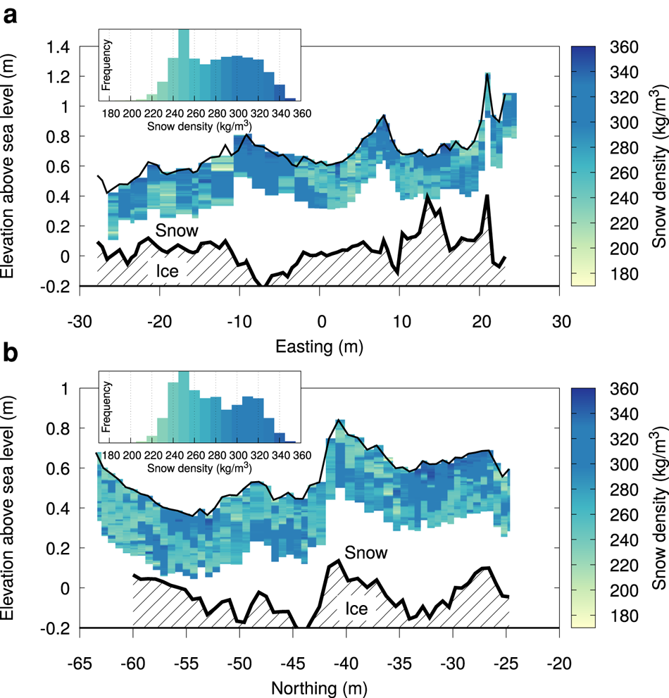
Fig. 8. Snow density in the upper ~30 cm of the snow cover from SMP, for the west–east transect (a) and the south–north transect (b) inside the TLS field at the ice station PS81/517. The insets show a histogram of all densities recorded by the SMP, binned with bin widths of 10 kg m−3. The thin black solid line shows the snow surface from TLS and the thick black line shows the approximate transition between snow and ice, determined using Magnaprobe combined with the TLS data.
Since snow deposition in a wind dominated environment is known to be inhomogeneous and governed by dune formation (Trujillo and others, Reference Trujillo, Leonard, Maksym and Lehning2016; Sommer and others, Reference Sommer, Wever, Fierz and Lehning2018), it is likely that the SMP measurements depict overlapping dunes that formed during several accumulation events. Varying wind speed during accumulation or drifting snow events controls the density of accumulations (Groot Zwaaftink and others, Reference Groot Zwaaftink2013). Sommer and others (Reference Sommer, Wever, Fierz and Lehning2018) show dunes forming in level terrain during drifting snow with an accumulation depth up to 20–30 cm. For sea ice, the presence of pressure ridges may cause very localized increases in the depth of accumulation in drifting snow conditions (Trujillo and others, Reference Trujillo, Leonard, Maksym and Lehning2016; Liston and others, Reference Liston2018).
Snow on sea typically contains a basal layer with coarse depth hoar crystals (Arndt and Paul, Reference Arndt and Paul2018), which is not sampled by the instrument. We therefore interpret the bi-modal distribution as resulting from the density variations in the overlapping wind slabs covering the depth hoar layer.
Buoy data
At both ice stations PS81/506 and PS81/517, an AWS buoy and an IMB were installed and left on the ice after the ship departed. Figure 9a shows the snow depth measured by the AWS, the snow depth determined by the IMB, and the precipitation time series from MERRA-2 for ice station PS81/506. Unfortunately, this AWS buoy survived for only about a month, such that the time span for comparison is short, relative to the IMB. We find an increase in IMB snow depth of about 0.1 m, peaking on 25 July. During the same time, the AWS data also exhibit a bump in snow depth. The MERRA-2 data confirm a precipitation event around the same date. The SPC data show an increase in the cumulative logarithm of counted particles, consistent with precipitation. However, the SPC data also suggest that blowing snow frequently occurs during periods with no or little precipitation in the MERRA-2 data. We find that the precipitation events from MERRA-2 are relatively poorly represented by changes in the snow depth at the IMB. Some precipitation periods from MERRA-2 do not correspond to a snow depth increase.

Fig. 9. Data measured by the buoys installed at PS81/506 and MERRA-2 output, for (a) snow depth (HS) measured by the AWS and determined from the IMB, and data from the snow particle counters (SPC) shown as the cumulative sum of the logarithm of the recorded number of particles, and cumulative precipitation from MERRA-2. The SPC data are scaled between the bottom and top of the graph. (b) shows the air temperature (TA) and wind speed (VW) from both the AWS and MERRA-2. (c) shows the temperatures recorded by the IMB, masked by the manually determined interfaces. The depth is relative to the snow–ice interface upon installation of the IMB and indicated by a dashed line. The snow surface is indicated by a thin dashed line and flooding by a dotted line.
The IMB installed at ice station PS81/517 survived slightly over 2 months, whereas the accompanying AWS survived over 3 months. Figure 10a shows the snow depth as measured by the AWS and as determined from the IMB, as well as the cumulative precipitation from MERRA-2. Both snow depth measurements show no consistent accumulation of snow, in spite of about 70 mm of cumulative precipitation simulated by MERRA-2 for this period. However, we find good correspondence between observed drifting snow by the SPCs and precipitation input from MERRA-2.

Fig. 10. As Figure 9, but for PS81/517. Flooding could not be determined in the data from this IMB.
As for PS81/506, we find a poor correspondence between both snow depth measurements, and between the snow depth measurements and the MERRA-2 precipitation. We also find that the wind speed often exceeds typical thresholds for the occurrence of blowing snow (Figs 9b and 10b), and blowing snow was indeed recorded by the SPCs (Figs 9a and 10a). The data from the SPCs show regular drifting snow events during austral winter, subsiding towards spring and austral summer.
These results illustrate that some precipitation may not accumulate on the sea ice, while it is being transported by wind. Irregular snow depth measurements, such as the snow depth bumps visible around August 21 at PS81/517 (Fig. 10a) could also be interpreted as caused by the migration of snow dunes under the sensor. Erosion followed by deposition under drifting snow conditions can lead to higher density and thus a net snow height reduction. Drifting snow loss in leads (Leonard and Maksym, Reference Leonard and Maksym2011) and drifting snow sublimation (Wever and others, Reference Wever2009) are processes that can cause discrepancies between precipitation and actual snow accumulation on sea ice. Furthermore, PS81/506 was shown to exhibit flooding. Upon wetting of the snow, enhanced wet snow settling (Colbeck, Reference Colbeck1979; Marshall and others, Reference Marshall, Conway and Rasmussen1999) can hide the snow depth increases resulting from snowfall. These results once again suggest uncertainty in snow accumulating on sea ice due to blowing snow eroding existing snow and/or preventing fresh snow accumulating.
Figures 9b and 10b show the daily average air temperature and wind speed from the AWS and MERRA-2 for ice stations PS81/506 and PS81/517, respectively. Note that the buoy's data were not assimilated by MERRA-2. For PS81/506, the time series from the AWS is too short to draw conclusions about the suitability of MERRA-2 to drive the model simulations in this study. PS81/517 shows, however, that the daily average air temperature measured by the AWS corresponds very well with MERRA-2 simulated air temperature. The wind speed observed at the AWS is lower than simulated by MERRA-2, since the simulated wind speed is referenced at 10 m above the surface, whereas the measurement height of the wind speed at the AWS on installation was 2.50 ± 0.03 and 2.27 ± 0.03 m for PS81/506 and PS81/517, respectively. The temporal variability shows a good correspondence between the AWS and MERRA-2.
Figures 9c and 10c show the temperature distributions from the temperature sensor string from the IMB through the snow–sea ice for ice stations PS81/506 and PS81/517, respectively. The manually determined interfaces were used to mask out the temperature data from air and ocean. The IMB installed at PS81/506 showed flooding of >5 cm above the snow–ice interface from 19 October onwards. Flooding was not detected in the IMB data for PS81/517.
In austral winter, the daily average air temperature for PS81/506 was as low as −35°C. These cold episodes around 3 and 23 August are reflected by drops in temperature in the snow and upper part of the sea ice. Consequently, the sea-ice thickness for PS81/506 increased from 0.77 on 15 July to 0.90 m on 8 September (Fig. 9c). In austral summer, the daily average air temperatures remain mostly just below the melting point (Fig. 9b). Combined with some solar radiation input, snow melt probably occurred at PS81/506, given the temperatures close to 0°C (Fig. 9c).
At PS81/517, we find similar cold episodes as for PS81/506, albeit with higher temperatures. The sea-ice thickness increased from 50 cm in the beginning of August to 57 cm on 8 October, when the last useable data were received. In early October, a decrease of snow depth is indicative of snow melt. Interestingly, the snow depth measured by the IMB shows a stronger decrease than at the AWS. This may be because the shallower snowpack and thinner ice at the IMB site allowed warming of the ice below to near the melting temperature, while at the AWS, the greater ice thickness delayed warming of the ice below, and thus may have delayed snow melt as absorbed heat continued to be conducted away to warm the colder ice below. The decrease of snow albedo upon wetting additionally provides a positive feedback loop here. This suggests considerable spatial variability in snow melt on small scales. On the other hand, heating of the thermistor string with solar radiation could have melted snow around the thermistor string. This makes deriving snow layer thickness from the thermistor string less reliable than the sonic ranger snow depth measurement used at the AWS.
1-D simulations
First, we performed 1-D simulations with the SNOWPACK model to simulate the temporal evolution of the floes for the two ice stations for which IMB data are available, and to compare the simulations with that data. We set initial sea-ice thickness and snow thickness corresponding to the thicknesses measured when the buoys were installed, and use meteorological forcing data, including precipitation, from MERRA-2. This simulation describes the scenario where the IMB data would be used as a point representation of the evolution of the entire sea-ice floe.
Figure 11 shows the temperature and liquid water content (LWC) from the simulation for PS81/506. Note that some numerical oscillations arise from the use of the Crank–Nicolson scheme, as discussed by Wever and others (Reference Wever2020). We attribute it to the interplay between oscillations in the solution for the brine salinity, which in turns impacts the local thermodynamics processes. However, it is not likely that the simulated flooding processes are impacted by these oscillations and we assume the effect of those oscillations on results presented here to be small.

Fig. 11. Results for the 1-D simulation for the IMB installed at ice station PS81/506, for (a) temperature, and (b) volumetric LWC. The depth is relative to the initial snow–ice interface, which is indicated by a dashed black line. Sea level is denoted by a solid black line, and the sea-ice top, flooding level and sea ice bottom determined from the IMB data are shown by a dotted, solid and dashed cyan line, respectively. In (b), dry snow is colored gray.
August and the first half of September show little snow accumulation, followed by an accumulation event around mid-September, and another accumulation period in the first half of October. This corresponds very well with the observations from the IMB (Fig. 9c). However, the simulations show up to 10–20 cm more snow on the sea ice than the buoy data in August and September. In early October, the observed snow depth matches the simulated snow depth, after which the discrepancy returns to an overestimated simulated snow depth of about 10–20 cm. Boisvert and others (Reference Boisvert2020) demonstrate for several reanalysis products that the uncertainty of individual precipitation events is large, even when the timing is accurate. Also, simulated snow density plays a role here. From 1 August to 1 October, when flooding is still inconsequential, the average simulated snow density of the uppermost 30 cm for PS81/506 is 259 kg m−3, which is lower than found in the SMP measurements during ice station PS81/517.
We find that low air temperatures cooled down the sea ice as well, particularly in August, the first half of September and the beginning of October. However, the depth to which the low temperatures reach is underestimated by the simulations. The modeled low temperatures are mainly restricted to the snow layer, resulting from low thermal conductivity (and thus high insulation) of the snow layer. In contrast, the IMB data show a significant cooling of the ice. This discrepancy may originate from the overestimated snow depth in the simulations. We also found that initializing the simulations with higher salinity (see Fig. S7 in Supplementary material) gives slightly enhanced cooling of the uppermost ice layers below the snow cover, which could also be an explanation for this discrepancy.
The ice thickness increased by 0.13 m after installation of the IMB (Fig. 9c). In the 1-D simulations, the ice thickness increased by 5 cm, which is less than in the observations. This discrepancy could result from an overestimated simulated snow depth, the higher ice temperatures simulated for the sea ice or an overestimation of the ocean heat flux. From October onwards, both the simulation and the IMB data show thinning of the sea ice.
The simulation suggests that the accumulation events and bottom sea-ice melt caused a significant flooding of the sea ice, indicated by the sea level crossing the snow–ice interface upon installation of the IMB, starting on 1 September. This is reflected by the LWC, as shown in Figure 11b. Initially, only low values of 5$\percnt$ LWC or less can be found above the installation reference level, caused by capillary suction. However, in October, the sea ice is simulated to flood, causing filling of the pore space and values of liquid water content exceeding $30\percnt$
 . The flooded layer in the simulations is approximately three times deeper than the IMB observations indicate.
Figure 12 shows the temperature and LWC of the simulation for PS81/517. In agreement with the IMB data, during the time period the buoy was active, snow and ice thickness remained fairly constant (Fig. 10c). The model overestimates snow depth from 5 to 10 cm up to mid-September, after which the discrepancy grows to around 15 cm. The strong decrease in buoy-observed snow depth in October is not reproduced in the model.

Fig. 12. Results for the 1-D simulation for the IMB installed at ice station PS81/517, for (a) temperature, and (b) volumetric LWC. The depth is relative to the initial snow–ice interface, which is indicated by a dashed black line. Sea level is denoted by a solid black line. The ice–ocean interface from a simulation with an ocean heat flux of 2 W m−2 is shown by a black dotted line. The sea-ice top and sea-ice bottom determined from the IMB data are shown by a dotted and dashed cyan line, respectively. The IMB data did not reveal the occurrence of flooding. In (b), dry snow is colored gray.
During warm phases, as for example around 27 August, 4 and 18 September, the snow height slightly decreases. This results from increased snow settling when the snowpack heats up, even though no meltwater was produced. Furthermore, the initial freeboard is close to 0 cm. This was observed upon installation of the IMB (see Fig. 7), but also confirmed by the hydrostatic balance applied in the 1-D SNOWPACK simulations, positioning the sea level at the initial snow–ice interface (solid and dashed line in Fig. 12).
The 1-D simulation shows an ~20 cm increase of the sea level inside the model domain, which would indicate the possibility of flooding. However, the simulations only produce a substantial layer with very high values of LWC (>30%) towards the end of the simulation period. Apparently, the simulation suggests that the flooded layers quickly turned into 15 cm thick snow-ice due to refreezing. However, neither flooding nor snow–ice formation could be detected in the IMB data.
Earlier it was noted that the 70 mm cumulative precipitation in MERRA-2 did not correspond to a consistent snow depth increase in the buoy data. Interestingly, the 1-D simulation also does not show a significant snow depth increase. In the simulations, flooding triggers an additional snow settling in the model, thereby compensating for the accumulation from the MERRA-2 precipitation. However, indications for flooding were not found in the IMB data, suggesting that not much mass from snowfall was added in during this period. Later it will be shown that also spatially distributed simulations for this floe, which were initialized with much thicker ice, only produce shallow flooding (<5 cm). Other factors could be that MERRA-2 overestimates snowfall, or drifting snow loss in leads or wind erosion inhibits accumulation on the sea ice.
On 1 October, high snowmelt rates during a warm phase with daily average air temperatures around 0°C (see Fig. 10) that persists for 2 weeks, creates high values of LWC in the snowpack above sea ice. This is partly caused by sea level being close to the snow surface, reducing the hydraulic pressure gradient. However, the layer with the high LWC increases in depth compared to earlier in the simulation. When melt rates are high, the strong decrease in hydraulic conductivity between the snowpack and underlying ice slows down the drainage of the meltwater. Around this time, the IMB data connection was lost. We hypothesize that external conditions (liquid water damage or floe breakup) are the likely cause of failure of the buoy.
Recall here that the IMB data showed evidence for an increase in ice thickness of about 7 cm, whereas the simulation with an ocean heat flux of 8 W m−2 show a decrease for most of the simulated period. Since Robertson and others (Reference Robertson, Padman and Levine1995) suggested that the ocean heat flux could be as low as 2 W m−2 in the Western Weddell Sea, we redid the simulation for PS81/517 with an ocean heat flux of 2 W m−2. Figure 12 shows the bottom of the sea ice relative to the reference level by a dotted line, which indicates an increase of sea ice thickness of 6 cm up to the end of September, which is in close agreement with the IMB data.
Spatially distributed simulations
To assess the influence of spatial heterogeneity in sea ice and snow thickness on the mass balance of the sea ice, we performed spatially distributed simulations using Alpine3D. These simulations run SNOWPACK simulations for each grid cell, without considering lateral exchange of heat and brine/flooding, but with a consistent hydrostatic balance such that the relative vertical positions of the individual grid cells do not change (see Floe Buoyancy section).
Since we found that the conditions at the installation location of the IMB where not necessarily representative for larger scales, we additionally performed 1-D SNOWPACK simulations where we initialized SNOWPACK with the TLS field-averaged snow and ice thicknesses of the fields used to initialize Alpine3D (see Figs 4a, b and 5a, b, for PS81/506 and PS81/517, respectively). Note that these floe-averaged 1-D simulations thereby differ from the simulations shown in the previous section, which were initialized with the snow and ice thickness measured at the installation sites of the IMBs.
Figures 13a and 14a show the temporal evolution of snow and ice thickness, and the flooded layer when flooding occurred, for both the floe-averaged 1-D SNOWPACK simulation and the distributed Alpine3D simulation. The areas are colored based on the average positions the interfaces between air–snow (surface) snow–ice, and ice–ocean (bottom). The unflooded snow layer is defined as the part of the model domain having at least one out of three neighboring layers with a dry snow density (i.e. density excluding water) <700 kg m−3. Individual ice layers inside the snowpack are thereby still considered snow. Such ice layers can easily form after refreezing of water accumulating on layer transitions with contrasting microstructural properties (particularly grain size and density) inside the snowpack (Wever and others, Reference Wever, Würzer, Fierz and Lehning2016). The flooding layer is defined as saturated snow layers, which corresponds to a bulk density >900 kg m−3 with a LWC larger than $21.7\percnt$ . The latter requirement is congruent with our definition of unflooded snow layers. Namely, when LWC exceeds $21.7\percnt$
 , the dry snow density must be <700 kg m−3. The remaining layers are considered ice. Figure 15 shows the simulated and observed depth of the flooded layer for ice station PS81/506, which likely experienced flooding based on the simulations and the IMB data.

Fig. 13. Results for (a) the 1-D SNOWPACK simulation initialized with average snow and ice thickness of the fields used to initialize the spatially distributed Alpine3D simulation and (b) the spatially distributed Alpine3D simulation for ice station PS81/506. The depth on the y-axis is relative to sea level. Gray areas indicate the snow (defined as a dry snow density lower than 700 kg m−3) and blue areas indicate the presence of flooding (defined as a bulk density larger than 900 kg m−3 and a LWC larger than $21.7\percnt$ ). The remainder of the domain is considered ice and colored in cyan.

Fig. 14. As Figure 13, but for PS81/517.

Fig. 15. Temporal evolution of the depth of the flooded layer for ice station PS81/506, defined as (for the simulations) layers with a bulk density exceeding 900 kg m−3 and LWC exceeding $21.7\percnt$ , and (for the IMB data) determined from the thermistor string response. The cyan and yellow dashed line show results from a distributed simulation where precipitation was decreased by 25% and the ocean heat flux was reduced to 5 W m−2, respectively.
For ice station PS81/506, where the IMB was installed in snow and ice thickness representative for the floe (Fig. 6), the floe-averaged 1-D simulations are very similar to the distributed simulations up to early October. From October onwards, we find that the floe-averaged 1-D simulations calculate a deeper flooded layer compared to the distributed simulations (Fig. 15). Consequently, snow depth is lower in the floe-averaged 1-D simulations, since flooded layers are not considered snow layers. Also the surface height with respect to sea level decreases (see Fig. 13), in spite of continuing accumulation (Fig. 9a). This is mostly a result of the added weight of the flooded layer pushing the sea ice deeper in the water. Additionally, saturated snow compacts more under the presence of liquid water. Figures 4a, d, g show that initially, the snow depth increases due to precipitation, but between 1 November and 1 February, the snow depth decreases since flooding occurs and flooded snow layers are not considered snow. The decrease is found for the majority of the floe, since flooding is widespread over the floe. The combined snow and ice thickness increases slightly over time (Figs 4b, e, f), because the basal ice melt is compensated by snowfall, but patterns of spatial variability remain largely unaltered.
The depth of the flooding layer in the distributed simulations corresponds well with the depth derived from the IMB data. We now analyze the spatial distribution of flooding, since flooding is spatially variable (see Figs 4f, i). From Figure 13, it is clear that flooding is present in at least one pixel around mid-August and mid-September. However, the fractional pixel count of pixels exhibiting flooding, shown for three thresholds of flooded layer depth (0, 5 and 10 cm) in Figure 16, illustrates that up to mid-October, flooding was restricted to <10–20% of the area and it is possible that flooding did not occur at the location where the IMB was installed. Around mid-October, there is a sharp increase in the flooded area, peaking at $95\percnt$ on 26 December 2013. The flooded layer depth is substantial, since the majority of pixels reach 10 cm flooded layer depth. Based on this, we conclude that the timing of the onset of flooding seems to correspond well with the IMB, within a one-week time span. Note that the simulations immediately allow for flooding to start since hydraulic conductivity is always non-zero for numerical stability. The rate of flooding in the simulations is controlled by the increase in pressure head at the bottom of the domain and the hydraulic conductivity throughout the domain. Figure S8 in Supplementary material shows that when simulations are initialized with higher salinity, the rate with which flooding depth increases slows down. When flooding initiates, the high salinity brine is first to enter the snow matrix, being replaced by ocean water with lower salinity. To maintain thermal equilibrium in the brine, brine volume decreases, in turn decreasing hydraulic conductivity.

Fig. 16. Temporal evolution of the fractional area of pixels where flooding is detected, defined as layers with a bulk density exceeding 900 kg m−3 and LWC exceeding $21.7\percnt$ for ice station PS81/506, for thresholds of a minimum flooded layer depth of 0 cm (solid lines), 5 cm (dashed lines) and 10 cm (dotted lines).
In reality, negative freeboard may exist without flooding for extended periods of time when hydraulic conductivity is negligible small or there are no cracks or deformations in the sea ice. Since controlling flooding only via hydraulic conductivity in models was found to not be an adequate approach (Maksym and Jeffries, Reference Maksym and Jeffries2000), our model assumption which always keeps minimal hydraulic conductivity can be considered a pragmatic approach to allow for flooding when the model is not considering deformations and crack formation which can initiate flooding. However, as discussed above, the flooding rate remains a function of hydraulic conductivity in the model, which varies based on the simulated state of the sea ice. It is thereby an important source of uncertainty.
For ice station PS81/517, Figure 14 shows that the distributed and floe-averaged 1-D simulations produce very similar results, and both confirm very little change in ice and snow thicknesses and liquid water content during the observational period. The earlier depicted scenario from the 1-D simulation using snow and ice thickness at the IMB site of substantial flooding which quickly transformed into snow ice due to refreezing is not supported here, given the rather constant ice thickness. The ice and snow thickness for the TLS area were much higher than for the area where the IMB was installed (see Fig. 7). Since the freeboard was close to 0 cm, the small increase in snow depth on top of thick ice (around 1.80 m) results in a shallow flooded layer. Figure 16 shows that there is a substantial difference in the fractional flooded area considering a minimum layer depth of 0 cm versus 5 cm, indicating that flooding is widespread, but very shallow (see also Figs 4f, i). The much thicker snow cover would likely inhibit refreezing compared to simulations with initial conditions from the IMB site (Fig. 12). Moreover, it is difficult to detect very shallow flooding in the IMB data, which had a sensor spacing of 2 cm. Figures 5a, d, g show that the snow depth increases throughout the simulation period and the initial spatial variability remains unchanged in the simulations. The combined snow and ice thickness (Figs 4b, e, h) also remains unaltered, both in amount and its spatial distribution.
Some care has to be taken to interpret the IMB as representative for the floe as a whole. Nevertheless, we are confident that the IMB for floe PS81/506, which exhibited substantial flooding, was installed in an area with average snow and ice thickness (Fig. 6). Also the freeboard is comparable between sites. In the following, we assume that we can interpret the IMB as being representative, and the flooding observed at the IMB as representative. The simulations suggest that distributed simulations more accurately capture flooding of the sea ice than 1-D simulations. Thick sea ice can add buoyancy to the floe and prevent flooding of shallower parts. This confirms previous studies that on the point scale, the hydrostatic balance cannot be assumed. Furthermore, the modeling results suggest that the 3D shape of a sea-ice floe needs to be considered for accurately calculating the effect of flooding on the mass balance. The flooding layer depth in the simulations was found to be spatially variable (see Figs 4f, i, 5f, i). This variability impacts the mass added to the snow from flooding, and thereby the hydrostatic balance of the floe. When comparing flooded layer depth from the IMB data with the model results, we also need to consider that the ice thickness in the TLS field on PS81/506 was found to be slightly thicker than on the floe-scale walk (Fig. 6), which would be associated with an underestimation of the flooding. This may compensate for the higher snow load that is added over the simulation period, which was suggested by the 1-D simulation (Fig. 11).
Cross-checking 1-D and distributed simulations
The 1-D simulations enforced hydrostatic balance, whereas the distributed simulations were set-up to calculate changes in buoyancy based on the initial positioning of the sea-ice floe relative to sea level. If the initialization of sea level obeys hydrostatic balance, the Alpine3D simulations maintain hydrostatic balance. Then, the distributed simulations can be initialized to mimic a 1-D simulation, by prescribing exactly the same initial conditions for each pixel and setting the initial conditions exactly the same as for the 1-D simulation.
Figures 17a, b make exactly this comparison. We find that the simulations are nearly identical, suggesting a correct implementation of the sea ice version and hydrostatic balance in the Alpine3D model. Differences can arise in the first place because the distributed simulations update the hydrostatic balance and meteorological forcing data on an hourly time step, whereas the SNOWPACK model assesses the hydrostatic balance and meteorological data on 15 min time steps. Other differences could arise because of minor implementation differences between SNOWPACK and Alpine3D.

Fig. 17. As Figure 13, but where (b) shows the distributed simulation enforcing hydrostatic balance, with each pixel initialized with the floe-averaged initial conditions to mimic the 1-D simulation. (c) is as (b), but with updating observed freeboard using changes in buoyancy. (a) is identical to Figure 13a, but repeated here to allow for a direct comparison. Definitions of color coding as shown in Figure 13.
As another test, we added simulations using Alpine3D, where again each pixel is initialized exactly the same, with the floe-averaged snow and ice thickness, but now with average sea level as derived from freeboard observations using TLS and GEM2 data. We can interpret this setup as compared to a modification of the 1-D simulation where instead of enforcing hydrostatic balance, we would initialize with observed freeboard as well. Figure 17c shows the simulation result. We find this approach to be inadequate, as only a very shallow flooding layer appears in December, when the ice layers sink below the sea level, denoted by 0 m depth. However, this is much later than the onset of flooding seen in the IMB data, which was around mid-October, and also shallower than seen in the IMB data. These results suggest that accurate determination of onset and amount of flooding requires an explicit consideration of the spatial variability in snow and ice thickness. It also plays a role that once flooding starts, weight is added to the system, which further enhances the flooding. The differences in results from 1-D versus spatial simulations do not solely stem from the fact that the point measurements at a buoy site do not accurately represent average snow and sea-ice mass, but also that the they do not necessarily capture the floe-scale variability in susceptibility for, and amount of flooding, as shown in Figures 4f, i, 5f, i.
Limitations of the simulations
The simulations presented here have various limitations. There are processes we have not considered, such as lateral heat, lateral brine flow/flooding and floe bending. However, lateral flow processes likely constitute small effects, given the large spatial extents of several hundreds of meters, compared to the typical ice thickness of a few meters. Floe bending could have a larger effect, given the spatially variable flooding occurring in the simulations and uneven snow distributions. When floe bending occurs, flooding is expected to be more localized, but deeper. Furthermore, several processes, such as ice deformation and crack formation, are difficult to incorporate in this model framework. If multiple pressure ridges would form near or at the floe during the period we simulated, this could have a profound impact on the potential for flooding. We also initialized the snow and sea ice with spatially constant snow and ice density, whereas this in reality may not hold. This would impact the initial hydrostatic balance we calculate for the floe.
Other uncertainties could be overcome if other data sources were available. Basal melt, controlled by ocean heat flux, has earlier been associated with flooding (Lytle and Ackley, Reference Lytle and Ackley2001). Changes in ocean heat flux could be easily prescribed in the model, but it is generally not a well-constrained variable. We also relied on MERRA-2 precipitation to determine accumulation. The total accumulation on the sea ice poses a strong control on the flooding process. MERRA-2 performs reasonably well for the Weddell Sea area compared to other reanalysis products (Boisvert and others, Reference Boisvert2020). However, the role of drifting snow erosion, and subsequent drifting snow sublimation (Wever and others, Reference Wever2009) and mass loss in leads (Leonard and Maksym, Reference Leonard and Maksym2011), cause a poorly constrained relationship between precipitation and snow accumulation on sea ice (Webster and others, Reference Webster2018). We also discussed the role of initial salinity on hydraulic conductivity when flooding initiates in the simulations. Even though initial salinity on other parts of the floe are known from other research activities (Tison and others, Reference Tison2017), the temporal evolution after the floe visit is unknown. In Wever and others (Reference Wever2020), it is discussed that the description of brine salinity dynamics in the SNOWPACK model is incomplete, particularly since it does not describe convective brine dynamics upon cooling (Griewank and Notz, Reference Griewank and Notz2013). That could lead to an overestimation of bulk salinity in the model, compensating for an initially lower salinity in the model than observed.
To provide an estimate of the effect of some of the above mentioned uncertainties on the results, we include two additional simulation results for PS81/506 as shown in Figure 15. In the first, we forced the simulation with 25$\percnt$ less precipitation. In the second, we reduced the ocean heat flux by 3 W m−2 from 8 W m−2 (as used throughout this manuscript) to 5 W m−2. We consider these sensitivity experiments to roughly cover the typical uncertainties in those variables. We find that precipitation amounts have a much stronger effect on simulated flooding than the ocean heat flux. In Figures S7, S8 in Supplementary material, we compare 1-D simulations with initial bulk salinity of 1.75 g kg−1 in layers below sea level to simulations with a higher initial bulk salinity of 5 g kg−1 in those layers. We find that the higher salinity leads to lower hydraulic conductivity and consequently lower flooding rates. As mentioned earlier, this can be attributed to the high salinity brine being replaced with ocean water with a lower salinity in the ice matrix upon flooding. To maintain thermal equilibrium, the brine volume decreases. We also find that with higher initial salinity, the sea ice remains thicker and flooding layer depth is reduced (Fig. S8 in Supplementary material). However, it is important to note here that only considering flooding from the perspective of hydraulic conductivity through the ice is inadequate, since the presence of cracks is an important control on flooding as well (Maksym and Jeffries, Reference Maksym and Jeffries2000).
Conclusion
The effect of floe-scale spatial variability of snow and ice thickness on the mass and energy balance of sea ice is relatively poorly known. We used in situ, high spatial resolution datasets of snow and ice thickness, and IMBs and automatic weather stations buoys, to assess the temporal evolution of two sea-ice floes using the IMB data and numerical simulations. Data were collected during the AWECS campaign on board R/V Polarstern in the Weddell Sea near Antarctica in austral winter 2013. Analyzing data from three floes, we found that several methods for measuring snow and ice thickness over different parts of a floe yield relatively consistent results for their distributions. However, point locations, for example where an IMB was installed, were not necessarily representative for the floe scale. Also, the results confirm that individual points cannot be expected to be in hydrostatic balance, which means that they may not be flooded if buoyed up by surrounding ice.
The 1-D SNOWPACK model and its distributed variant Alpine3D were used to simulate the temporal evolution of two floes. We compared three types of simulation setups: (i) initial snow and ice thickness as observed upon IMB installation, (ii) initial snow and ice thickness as floe averages, determined from laser scanning and electromagnetic surveying and (iii), spatially distributed simulations exploiting the 3-D fields obtained from the floe.
For one ice station, with first-year ice, the IMB recorded substantial flooding of the sea ice. This IMB was installed in snow and ice thickness that was representative for the floe scale. However, assuming hydrostatic balance for 1-D simulations was found to produce approximately three times more flooding than observed at the IMB site, confirming previous studies indicating that hydrostatic balance does not necessarily hold on the point scale. Distributed simulations which were initialized with observed freeboard were found to provide a better agreement with the IMB data in terms of onset and amount of flooding than the 1-D simulations. Thicker ice can provide more flotation such that more snow needs to accumulate to trigger flooding. The simulations also showed spatially variable flooding depths, indicating a variability in flooding susceptibility of the floe. Once flooding starts, the added mass from flooding can enhance the flooding. Distributed simulations explicitly take aforementioned effects into account. Since the amount of flooding provides a potential considerable positive mass balance upon refreezing, it is an important notion that a 1-D simulation based on initial snow and ice thickness at an IMB may overestimate the amount of flooding considerably.
The 1-D simulation for the other ice station with usable IMB data, which was a multi-year floe, suggested flooding and quick refreezing leading to snow–ice formation of up to 15 cm. The distributed simulations, which were initialized with observations showing much thicker snow and ice than found at the IMB site, exhibited wide-spread flooding mostly constrained to a shallow layer (<5 cm). Refreezing was inhibited by a thick snow cover of around 70 cm. The IMB data did not show indications of flooding or snow–ice formation.
Snow depth changes derived from the IMB were found to not be necessarily consistent with the snow depth changes from a nearby AWS, probably related to the uneven accumulation of snow on the sea-ice floe under the presence of drifting snow conditions. We also found that the snow depth does not necessarily increase when precipitation occurred in the MERRA-2 reanalysis data. The simulations partly explain this as settling and enhanced settling of wet snow upon flooding counteracting accumulation. However, snow particle counters at the AWS show the abundance of drifting snow conditions. Drifting snow loss in leads and drifting snow sublimation likely play a role as well, but these processes are not included in our simulations. Using MERRA-2 in our simulations ultimately overestimated the snow depth by up to 20 cm.
Overall, our results highlight the uncertainties associated with the interactions between the snow cover and the underlying sea ice, particularly where large spatial variability exists, and that caution is warranted when spatially extrapolating point measurements or point simulations to assess the overall mass balance of sea ice.
Supplementary material
The supplementary material for this article can be found at https://doi.org/10.1017/jog.2021.54
Data and source code availability
The snow pit data are accessible via Paul and others (Reference Paul, Arndt and Stoll2017). The AWS buoy and IMB data from PS81/506 are accessible via DOIs https://doi.org/10.1594/PANGAEA.933415 and https://doi.org/10.1594/PANGAEA.933417, respectively. The AWS buoy and IMB data from PS81/517 are accessible via DOIs https://doi.org/10.1594/PANGAEA.933425 and https://doi.org/10.1594/PANGAEA.933424, respectively. Data from the Terrestrial Laser Scanner, Magnaprobe, GEM-2 for PS81-503, PS81-506 and PS81-517 are accessible via DOI: https://doi.org/10.1594/PANGAEA.933584. SnowMicroPen data (PS81/517) are accessible via DOIs https://doi.org/10.1594/PANGAEA.933101 (original files) and https://doi.org/10.1594/PANGAEA.933603 (curated files). MeteoIO, SNOWPACK and Alpine3D are software published under a GNU LGPLv3 license by the WSL Institute for Snow and Avalanche Research SLF at https://gitlabext.wsl.ch/snow-models. The repository used to develop the model code used in this study can be accessed via DOI: https://doi.org/10.5281/zenodo.4560829. The exact model source code used in this study can be accessed via DOI: https://doi.org/10.5281/zenodo.4708266. The model simulations can be accessed via DOI: https://doi.org/10.5281/zenodo.4717809. The MERRA-2 data can be obtained via: https://goldsmr4.gesdisc.eosdis.nasa.gov/data/MERRA2/.
Acknowledgments
We thank the captain and crew of R/V Polarstern for their excellent logistical support during the expedition ANT-29/6 (AWECS). We also thank the cruise leader Peter Lemke for enabling our field work and all scientists on board who provided us a helping hand in the field when needed. We are also grateful to the Sea Ice Physics Group from the Alfred Wegener Institute in Bremerhaven, Germany, in particular Stefan Hendricks and Priska Hunkeler, who kindly provided GEM-2 data, and Sandra Schwegmann for collecting and preparing the Retro-Drilling dataset. We thank Martin Schneebeli and Michael Lehning from the WSL Institute for Snow and Avalanche Research SLF for loaning us the SnowMicroPen and supporting the project, respectively. Jack Landy and an anonymous reviewer are thanked for providing detailed and insightful comments which helped to improve the manuscript considerably. Nander Wever was funded by the Swiss National Science Foundation (SNSF) grant number P2ELP2$\_$ 172299 and Katherine Leonard by SNSF grant number PZ00P2$\_$
 142684. Katherine Leonard and Seth White were funded by US National Science Foundation (NSF) grant ANT-1142075. Ted Maksym was funded by NSF grant numbers ANT-1142075 and ANT-1341513. Eric Keenan is acknowledged for assisting in preparing the MERRA-2 reanalysis data.


 Open access