


1 Introduction
Glaciers advance and retreat in response to changes in mass balance induced by climate. Thus the reconstruction of past variations of glaciers from geological evidence or historical observations is an important tool for deductions about past climate, and indeed the major climate variations identified in the past have been named in terms of ice extent as “Ice Ages”, “Neoglaciation”, and “The Little Ice Age” (Reference Porter and DentonPorter and Denton, 1967;Reference Flint Flint, 1971;Reference Lamb Lamb, 1977). Similarly, current trends of advance and retreat and the potential for future changes are of interest with regard to engineering activities locally near the margins of present glaciers (Untcrsteiner and Nye, 1968;Reference Fisher and Jones Fisher and Jones, 1971; Reference BindschadlerBindschadler, 1980; Reference ReehReeh, 1983) and on a global scale with regard to changes in sea-level (Reference MeierMeier, 1984).
The quantitative relationship between the histories of glacier termini fluctuations and climate change is complicated by a time lag between climate change and glacier response. The time lag occurs because a climate signal appears as a mass-balance perturbation over the full length of a glacier. Information about it is transmitted down-glacier to the terminus at finite velocities over a range of distances from head to terminus and, therefore, arrives at the terminus spread out in time. Consequently, the position of a glacier terminus represents a weighted average over past climate extending back over a time interval sufficiently long that there is no memory of prior climate. This paper is about the length of the memory, which we denote by TM and define to be the time constant in an exponential asymptotic approach to a final steady state after a sudden change in climate to a new constant climate. The size of TM is important with regard to both interpretation of glacier fluctuations in terms of climate and prediction of future changes in glacier areas.
Observational information has not clearly established typical sizes for тм. During the first part of this century most glaciers experienced prolonged retreats. Syntheses of data by Reference PorterPorter (1986) and Reference ReynaudReynaud (1978, 1983) indicate that between 1950 and 1970 many of these glaciers experienced nearly synchronous reversals of their retreats. This observation implies that each glacier is dominated by short-term climate effects, perhaps on the order of a few decades. This view has been expressed by Reference LliboutryLliboutry (1971) andReference Jȯhannesson Jôhannesson (1986).
A number of computer-based numerical models are now capable of predicting the time-dependent response of a glacier to an imposed history of mass balance (e.g.Reference Budd and Jenssen Budd and Jenssen, 1975;Reference Mahaffy Mahaffy, 1976; Reference Bindschadler Bindschadler, 1982; Reference WaddingtonWaddington, unpublished). Because all essential physics can in principle be incorporated in such models, they have the potential for accurate prediction and are important computational tools for specific applications.
On the other hand, the broad understanding of glacier response and simple semi-quantitative methods for estimating TM has depended primarily on the analytical theory built up by Reference LliboutryNye (1960,1963ab,1965a,b) and reviewed by Reference LliboutryLliboutry (1971), Reference Paterson Paterson (1981), andReference Hutter Hutter (1983). This theory is based on a linearized treatment of ice motion and describes the adjustment of glaciers to changes in mass balance in terms of propagation and diffusion of kinematic waves. In simplest terms, this theory predicts that Tm is related to the glacier length I and the terminus velocity u(l) by

where the factor f is commonly assumed to be about 1/2 (Reference PatersonPaterson, 1981, p. 258). For typical glaciers (l ~ 1−20 km,u(l) ~ 1−10 m a−1), Tm is then predicted to be on the order of 102–103 years. This is the theoretical, long time–scale commonly thought to be representative of typical glaciers Reference Paterson(Paterson, 1981), but it appears to be longer than available observations would indicate.
Reference Jȯhannesson, Raymond and WaddingtonJohannesson and others (1989) have used a simple argument to find
where h is the thickness scale for the glacier and b(l) is the balance rate (negative) at the terminus. For typical glaciers (h ~ 100—500 m, −b(l) ~ 1—10 m a−1), Tm is predicted to be on the order of 101–102 years. This calls into question the theoretical long time–scale, and appears to be more consistent with observation.
Both of these estimates for TM are consistent with the notion that TM = TV, where TV is a volume time–scale that gives the time needed for a changed mass balance to produce the volume change between the corresponding initial and final steady states. The two estimates for TM differ in how the volume change is estimated.
In this paper our goals are as follows. We use results from linearized kinematic wave theory and time–dependent numerical models to show that TM = TV can be regarded as generally applicable with the consequence that TM may be estimated from continuity considerations applied to steady–state profiles without recourse to time–dependent calculations. We review the linearized kinematic wave theory to find a simple geometrical interpretation of the factor f in Equation (1a). The determination of TM from Equation (1a) appears to be sensitive to details of ice dynamics at the terminus, because this equation includes terminus velocity. Equation (1a) will give valid results only when proper attention is given to the factor f we show f itself depends on details at the terminus. We provide a broader derivation and justification for the estimate of TM given by Reference Jȯhannesson, Raymond and WaddingtonJohannesson and others (1989) expressed in Equation (lb) to show that it is free of details of the terminus motion and provides a theoretically more robust and simpler estimate of TM than does Equation (1a).
II Background
In Nature, the evolution of a glacier occurs as its upper surface is displaced by the combined effects of ice motion and surface mass exchange. As a computational problem, one must solve conservation equations of mass, momentum, and energy in the volume of the glacier, subject to boundary conditions describing the transports to the external surfaces, and constitutive statements describing the mechanical and thermal behavior of the glacier material. The problem in its full potential complexity has many ramifications, some of which have been discussed byReference Fowler and Larson Fowler and Larson (1980) and Hutter (1983).
We will assume a temperate valley glacier with atmospheric pressure on its upper surface, a time–independent ice–flow law, and a specified sliding distribution. Because of these assumptions, energy conservation need not be considered to calculate the ice motion. These assumptions eliminate many potentially realistic behaviors of glaciers such as could occur as a result of changes in temperature, of changes in water conditions in the ice or at the bed, of changes in the ice structure induced by strain, or of changes in bed structure by erosional or depositional processes. Any of these could affect the ice dynamics through the ice flow or basal slip laws, and it is well known that some of these processes can cause variations unrelated to mass–balance changes, for example, spectacular glacier surges.
Let x represent distance along the glacier running from zero at the head to l(t) at the terminus (Fig. 1). A suitable description of the geometry of a valley glacier is provided by the distributions along the valley length of bed elevation y 0(X), ice thickness h(x,t) and width of the ice surface depending on ice thickness w(x,h). The thickness h and length I may change with time I. From these quantities, one may derive the tangent of the bed slope β(x) = −d y b (x)/dx and the tangent of the surface slope

Fig. 1. Definition of geometrical parameters and boundary conditions in longitudinal and trails verse cross–sections.

The balance rate in terms of ice volume per unit area and time is described by b(x,t) and represents an average over the glacier width.
With these notations the flow may be described by the ice volume–flux distribution Q(x,t) subject to a one–dimensional continuity equation

and a flux–geometry relationship
Equation (3) describes mass conservation integrated over the area of cross–sections assuming a unique density for ice (Reference PatersonPaterson, 1981).
Equation (4a) must be evaluated to approximate momentum conservation subject to atmospheric pressure on the upper surface, the specified sliding distribution at the bed, and the ice–flow law. For small slopes (α << 1), constant density p, and no sliding, it is standard to take
where K = 2A(ρg)n/(n + 2), r = n, s = η + 2 depend on n and A of the flow law ![]() . This often–used equation exactly satisfies momentum conservation and boundary conditions for a parallel–sided slab. Effects of lateral variations associated with real cross–sections of a valley can be taken into account by introducing shape factors, which affect the values of K and the power of h (Reference NyeNye, 1965c; Reference BindschadlerBindschadler, 1982; Reference EchelmeyerEchelmeyer, unpublished). To account for longitudinal variations requires a more complete description of the geometry than is afforded by the local thickness and slope. Such a description would involve higher longitudinal derivatives such as
. This often–used equation exactly satisfies momentum conservation and boundary conditions for a parallel–sided slab. Effects of lateral variations associated with real cross–sections of a valley can be taken into account by introducing shape factors, which affect the values of K and the power of h (Reference NyeNye, 1965c; Reference BindschadlerBindschadler, 1982; Reference EchelmeyerEchelmeyer, unpublished). To account for longitudinal variations requires a more complete description of the geometry than is afforded by the local thickness and slope. Such a description would involve higher longitudinal derivatives such as

III. Memory Length In Relation To Linearized Theory
Linearized equations
Reference NyeNye (1960,1963a,b) formulated Equations (3) and (4) assuming small changes from a datum state. This enabled him to linearize the equations and to analyze several simple model glaciers. The procedures and some of the results have been nicely summarized by Reference PatersonPaterson (1981, chapter 12) and extended byReference Lliboutry Lliboutry (1971) and Hutter (1983, chapter 6).
Following these authors, the linearized equations are set down as follows. A datum glacier described by l
0, h0(x), Q0(x), and associated quantities w0(x) = w(x,h0) and a0(x) = β(x) – dh0(x)/dx is set up, so that it is in steady state with a balance–rate distribution b0(x); in other words, these quantities satisfy Equations (3) and (4) without time derivatives. Small deviations from this datum condition are described by ![]() and
and ![]() To first order in the changes, Equations (4) become
To first order in the changes, Equations (4) become
with u0 = Q0/w0h0. Equation (3) becomes

when Q and α are eliminated using Equations (2), (5), and (6). To find Equation (7), it is also necessary to assume that width w is independent of x and h. Also, the specific flux relationship Equation (4b) used to evaluate change of flux with A and a on the far right of Equations (6) neglects effects from the valley cross–section. While important effects come from changes in width with thickness and along the glacier length, these are not essential to the considerations developed here and are omitted for simplicity. In this case u defined above is the mean velocity over depth. (More generally it would be proportional to the mean velocity in a cross–section.)
Special considerations must apply near the terminus. If ice cliffs and calving termini are excluded, h and q both go to zero. However, at the terminus of a temperate glacier u does not generally go to zero.Reference Nye Nye (1963a) argued that near a terminus u must become independent of A, so that Q/w = uh. In effect this is sliding motion of a rigid wedge shoved from behind. It implies
Similarly, slope a cannot affect Q where h goes to zero, and consequently
The arguments leading to Equations (8a) and (8b) are crucial to the development in the next sections. From Equations (5) and (8), it is predicted that

Change in length and volume caused by a step change in climate
If there is a step change in balance rate from b0(x) to b0(x) + b 1(x), eventually a new steady state is reached. We are especially interested in the volume change because, as we shall see, it is intimately related to the time–scale needed to complete the length change. We shall utilize features of the new steady state that can be found from continuity considerations applied to the original datum length l o of the glacier. In the following we will frequently be concerned with averages over the length x = 0 to x = l0 and these will be denoted by.
In the final steady state the flux past the original terminus position x = l0 must be

(For discussion purposes, we will think of <b1> and Q1(l0) to be positive.) The change in thickness A1 at the original terminus position Z0 must reach a value sufficient to transport the new steady–state flux. Then Equations (9) and (10) predict

which is equivalent toReference Nye Nye (1963a, equation 11). We shall return to this equation frequently. Note that it predicts h1 at l0 is affected by the flow dynamics only through u0 l0 , i.e. the original sliding velocity at the original terminus. This result is forced by the linearization and the arguments leading to Equations (8). The change in length is also easily calculated, since the ablation in the area between l0 and l0 + l0 must melt the flux Past l0 given by Equation (10). This gives

to first order in the changes (Reference LliboutryNye, 1960, equation 40).
To calculate the change in volume, the distribution of thickness change over the full length of the glacier must be known. For the purpose of discussion we describe the essential aspects by
This defines a time–dependent factor f which gives the average thickness change in proportion to the thickness change at the original terminus. Later we will show that as t → ∞ this factor becomes the factor f appearing in Equation (la).
In Equation (13), f cannot be determined from continuity alone, but dynamics are required. In the linearized theory, it is necessary to solve Equation (7) employing the full distributions of C0, D0, and b1 along the length of the glacier, and we may think of f as a functional of C0, D0, and bv In these terms the volume change per unit width above the original terminus is
or by substitution of Equation (11)
To first order, V1 is also the change in total volume.
Kinematic waves and natural time–scales
Equation (7) describes the combined propagation and diffusion of thickness changes (Reference NyeNye, 1963a). We may identify two relevant time–scales:
These represent approximately the respective times to propagate or diffuse a disturbance over the full length of the glacier. The expressions on the far right relate these times to the time required for ice to traverse the length of the glacier at the speed u0. In Equation (15a) the parameter s’ must be given by s’ = <C0>/<u0>, which from Equation (6a) would be evaluated approximately as
In Equation (15b) the parameter r’ must be given by r’ =
<D0>/(l0<u0>), which from Equation (6b) would be crudely expressed as
where ∆y s is the elevation difference between the head and the terminus. For low bed slopes 〈h0 ~〉 ~ ∆ys and r' ~ 3. In this case TC and TD are approximately equal to 1/5 and 1/30 of the transit time for the ice, respectively. For high bed slopes TC has the same evaluation, but TD becomes longer.
A third time–scale related to the source term b1(x,Z) may be defined with a reference to a step change in balance rate from b0(x) to b0 + bx(x,t). An obvious choice is 〈h1(x,∞)〉/〈b1(x)〉, which when combined with Equation (14a) gives
T v is therefore the ratio of the ultimate volume change V1 (∞) to the total rate of volume addition by the new balance rate acting over the full original length l 0 of the glacier. We refer to it as the volume time–scale, since it describes the time required to accumulate the new steady–state volume by the changed mass balance neglecting any ice flow past the original terminus. Note that Tv can be evaluated from Equation (17a) without regard to any linearization assumptions. Equations (17a) and (14b) and the linearization expressed in Equation (11) give Tv as
It shows Tv is scaled to the time needed for ice to traverse the complete glacier length, if it were to move the complete distance at the speed of the terminus. This is much longer than the time scaling of TC and TD which is based on the average speed (Equations (15)). If f is similar to 1/s’ and/or 1/(π2 r'), then it appears
It is also clear that the time–scale TM for the glacier to reach a final steady state cannot be shorter than Tv (i.e. ![]() ). In this simple way we can understand the appearance of distinct short and long time–scales described by Reference NyeNye (1963a). Approximate long time–scale response of a glacier terminus An approximate time–scale for complete adjustment of a glacier terminus can be derived based on the supposition that perturbations in ice thickness are spread out rather quickly over the glacier length by propagation and diffusion in comparison to the full adjustment time–scale, as suggested by Equation (18). An order–of–magnitude analysis of Equation (7) using Equation (18) shows that, after a step change in mass balance, the shape of the thickness profile h1(x,t) is essentially constant for times t greater than TC or TD of Equations (15). Therefore, we make the tentative hypothesis that f(t) ≈ f(∞) in Equation (13). Note Equation (7) shows that for t = 0, ∂h
1(x,t)/∂t = b
1(x,t). Therefore, as t → 0, ƒ(t) → b1(l0)/〈b1〉, which for uniform b1 implies f(0) = 1. Later we expect f(t) to decrease, and only after some elapsed time (t < τc 0r τD) can f(t) ≈ f(∞) be true. Therefore, the following analysis is restricted to the late phase of the adjustment. The total rate of volume change above the terminus can be calculated from the total extra accumulation rate <b1
(x)>l0
minus the extra ice flux q1(l0,t) past l0
as given by Equation (9). Together with Equation (14a) and the assumption ƒ(t) = ƒ(∞), this gives
). In this simple way we can understand the appearance of distinct short and long time–scales described by Reference NyeNye (1963a). Approximate long time–scale response of a glacier terminus An approximate time–scale for complete adjustment of a glacier terminus can be derived based on the supposition that perturbations in ice thickness are spread out rather quickly over the glacier length by propagation and diffusion in comparison to the full adjustment time–scale, as suggested by Equation (18). An order–of–magnitude analysis of Equation (7) using Equation (18) shows that, after a step change in mass balance, the shape of the thickness profile h1(x,t) is essentially constant for times t greater than TC or TD of Equations (15). Therefore, we make the tentative hypothesis that f(t) ≈ f(∞) in Equation (13). Note Equation (7) shows that for t = 0, ∂h
1(x,t)/∂t = b
1(x,t). Therefore, as t → 0, ƒ(t) → b1(l0)/〈b1〉, which for uniform b1 implies f(0) = 1. Later we expect f(t) to decrease, and only after some elapsed time (t < τc 0r τD) can f(t) ≈ f(∞) be true. Therefore, the following analysis is restricted to the late phase of the adjustment. The total rate of volume change above the terminus can be calculated from the total extra accumulation rate <b1
(x)>l0
minus the extra ice flux q1(l0,t) past l0
as given by Equation (9). Together with Equation (14a) and the assumption ƒ(t) = ƒ(∞), this gives

The solution in terms of h1(l0,t) is

where Tv is defined as in Equation (17b). Therefore h1(l0,t) and the corresponding change in glacier length I1(I) approach their asymptotic steady–state values (Equation (11)) with an exponential time constant Tv (Equation (17)). In this simple way, one may expect Tv to correspond to the memory length TM, so
Together, Equations (17b) and (21) imply Equation (la), when f in Equation (la) is identified with ƒ(∞) appearing in Equation (17b). From Equation (13), ƒ(∞) ≃ 〈h 1(x,∞〉/h 1(l0,∞). We therefore discover that the factor f in Equation (la) has a simple geometrical interpretation as the ratio of thickness change averaged over the full length of the glacier to the change at the terminus. This is an important observation as we will see in the following sections.
Discussion
Reference PatersonPaterson (1981, p. 257 and 258) showed that a simple theoretical linear model of glacier adjustment developed by Nye (1963a) had the property that response time (here referred to as TM) was the time required for the volume change (here referred to as TV). Similarly, response times obtained from kinematic wave theory applied to real glacier profiles (Nye, 1963a, b, 1965a; Reference ReehReeh, 1983) have this property. Although these authors do not state it explicitly, it may be inferred by examining their figures and tables. The foregoing analysis explains these results in a simple way. We may expect that within the linearized kinematic wave theory Equation (21) is generally valid, of course subject to the validity of the underlying assumption about shape similarity of elevation–change profiles described by ƒ(t) = ƒ(∞) for TC or τD < t < ∞. This assumption will be tested in section IV, where we will also examine whether Equation (21) is valid for large climate changes requiring a fully non–linear model.
In this section we have not been concerned with the actual values of f(t), which will depend on the particular distributions of C0, D0, and b1 within the linearized theory, or on other dynamic parameters in more complex non–linear models. This question will be considered in subsequent sections. However, we point out here that the results from the linearized theory for adjustment time coming from Equations (15), (17), and (21), and encapsulated in Equation (la) require very explicit, detailed treatment of the terminus dynamics; u(l0) must be known and f certainly must also be sensitive to the details. This is unfortunate, since there is little glaciological understanding of terminus dynamics. Furthermore, it seems intuitively unnecessary; it seems unrealistic that terminus sliding velocity should have such strong direct influence on the response time of a glacier. We might anticipate that, although u(l0) and f are individually sensitive to terminus dynamics, in combination in Equation (la) they are not. This idea has not been previously enunciated, and we shall return to it.
IV. Time-Dependent Numerical Analysis Of A Model Glacier
In section III, we introduced the following concepts: a surface-elevation change profile factor f (Equation (13)) that relates elevation change at the terminus h1(l0,t) to the total volume change above the terminus V1(t) (Equation (14a)); similarity of elevation-change profile shapes f(t) ≈ f(∞) for t large enough); a volume time-scale TV (Equation (17a)), and the relationship of memory length TM to TV (Equation (21)). When these are introduced into the linearized theory, one finds Equations (14b), (17b), and (la). However, these are general concepts that can be discussed without regard to the linearized theory. In this section we examine their broader validity in the context of both a fully non-linear glacier-flow model and a linearization of it corresponding to the kinematic wave theory. We focus on two crucial questions: (i) ![]()
Description of the model
The model consists of Equations (3) and (4) with s = 3 and r = 5. The width w is assumed to be independent of x and h. In Equation (4b), a is calculated from Equation (2). In order to introduce a small amount of sliding at the terminus l 0, Equation (4b) is modified by addition of a second right–hand side term to become

Note that g(lg) = 1 and g(x) decreases monotonically to zero up–glacier from the terminus. Equation (22) and the first part of Equation (6a) indicate that u0(l0) = C0(I0) = ε,which is consistent with Equation (8a). Since ε = u0(ln) is small in comparison to the velocity in the interior of the glacier and g(x) approaches 0 near the glacier head, the extra term on the right will be negligible except close to the terminus. Throughout this paper, we will call this model the ε model.
The basal topography is chosen to be an inclined plane with slope β (Fig. 2) and the datum mass balance is chosen b0(x) = –a (constant) for l0/2 < x. We assume that the head of the glacier is a flow divide where ice thickness is non–zero. (For β = 0, this model may also be interpreted as a model of a two–dimensional symmetric ice sheet on a flat bed.) The side conditions consist of an initial condition specifying h(x,t = 0), the boundary condition q(x = 0,t) = 0, and a moving boundary condition at the time–dependent position l(t) of the terminus: h(l(t),t) = 0,
 , and a time–scale T = H/a, Equations (3) and (22), in non–dimensional form, become

Fig. 2. Geometry of model glacier. b0(x) = a (constant) for o < x < l 0/2 and
The steady–state thickness in the interior of the glacier is of the order of 1 and the maximum flux is 1/2. An order–of–magnitude estimate of the ratio of the velocity at the terminus to the maximum velocity in the interior for real glaciers is u0(l0)/u 0max ~ 1/10 (Nye, 1963a). The corresponding value of ε is ε = u0(l0) = C0(l0) = 0.05 for the model glacier considered here.
Equations (23) were solved numerically for ε = 0.05, 0.1, and 0.2 with the finite–difference model described byReference Waddington Waddington (unpublished) and with a numerical model based on the control–volume concept (Reference PatankarPatankar, 1980). In this section we will concentrate on the results for ε = 0.2, because they are easier to display graphically. Our conclusions apply equally well to the lower values of ε. The effect from variation of ε is examined in more detail in the next section.
Initial growth to steady state
In order to investigate perturbations from a steady state and the associated adjustment time, the steady state itself must be found. Figure 3 shows growth of the model glacier on a flat bed (β = 0) from near–zero ice thickness towards steady state. The time–scale to grow to steady state is shown in Figure 4, where the volume of the glacier
is shown as a function of time. For comparison, an exponential approach with time–scale T = 1 is shown. It is clear that the growth time–scale is close to 1 time unit (=H/a).

Fig. 3. Growth of model glacier (Equations (23)) from near–zero mass to near–steady–state at t = 4.0 for the steady mass–balance distribution of b0 = 1.0 for x/l0 < 0.5 and b0 = –1.0 for x/l0 < 0.5. Model parameter ε = 0.2. Curves are spaced in time by 0.1 time units. Dashed curve shows final steady state at t = ∞.

Fig. 4. Time variation of volume of model glacier growing to steady state (Fig. 3). Solid curve V(t)/V(∞). Dashed curve [1 – exp(t/T)] with T = 1.0 time unit (H/a).
Growth after a mass–balance perturbation
Starting with the steady–state profile hQ(x) in Figure 3, a mass–balance perturbation b1 = 0.01 was added at t = 0. Figure 5 shows the thickness perturbation h1(x,t) = h(x,t) – h0(x) at times t= 0, 0.2, 0.4, … time units. After t ≈ 0.4, the shapes of the profiles h1(x,t) are similar to the shape of h 1(x,∞), which supports the supposition f(t ≈ f(∞) that lies behind the derivation of Equation (19) and Equation (21). This supposition is confirmed more quantitatively in Figure 6 where f(t) is shown. Note that after t ≈ 0.4 approaches an asymptotic value, which for b1 = 0.01 is approximately equal to ε = 0.2. (The curves for the larger values of b1 will be discussed later in the text) Furthermore, Figure 7 shows that the model results for
and h1(l0,t) are both well approximated by exponential time variation with time constant ![]() time units (H/a) evaluated from Equation (17a). Therefore, Kquation (21) holds.
time units (H/a) evaluated from Equation (17a). Therefore, Kquation (21) holds.

Fig. 5. Response of the steady–state glacier shown in Figure 3 to a step change in climate A1 = 0.01. Curves show change in thickness h1(x,t))/H versus x for times spaced 0.2 lime units starting at the time of the step change in climate. The final curve, for t = 4.0 time units is indistinguishable from the final steady state h1(x,℞)/H. Curves derived from full model and from linearized kinematic wave treatment are also indistinguishable.
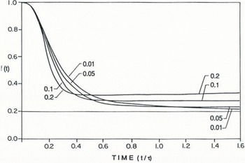
Fig. 6. Time dependence of f(t) for response to step change in climate for b1 = 0.01. 0.05. 0.10, and 0.20.

Fig. 7. Time variation of terminus thickness h1(10J) and volume change V1(t) induced by a step change in climate for the model glacier examined in Figures 3 and 5. Solid curves are given by the full model. Short–dashed curves are derived from the linearized kinematic wave theory, where results are distinguishable from the solid curves. Long–dashed curve is [1 – exp(t/Tv)] with V1(∞)/l0b1 = 1.06 lime units.
In order to test the validity of the linearized kinematic wave theory for this problem, the model was run in “linear mode”, which solves the linear perturbation equations for Q1(XJ) (Equations (5), (6), and (7)), instead of the non–linear equations for h = h0 + h1. The kinematic wave velocity C0 = (dq/dh)0 and the diffusion coefficient D 0 = ∂q/∂h were calculated from Equation (23b), and their distributions are shown in Figure 8. The calculated elevation–change profiles are almost identical to the results of the non–linear calculations (see Figs 5–7). Therefore, linearized kinematic wave theory yields results which are consistent with the non–linear equations, which is expected since b1 was chosen to be small. The corresponding time constants TC and TD Equations given by Equations (15) are 0.75 and 0.17, respectively.

Fig. 8. Distributions of non–dimensionalized kinematic wave velocity C0 and diffusion coefficient C0 corresponding to the steady state reached by the ε glacier–flow model in Figure 3. Dashed curves show the scaled distributions of C0 and D0 for the 1,8 model of Nye (1963a).
Discussion
The time–dependent analysis shows that f(t ≈ f(∞) for t > 0.4τ V (Fig. 6) and τM ≈ TV(Fig. 7), supporting the general validity of Equation (21). It also gives numerical values for the factor f(∞) (Equation (13)) approximately equal to ε. Thickness change is concentrated near the terminus and the profiles are distinctly concave (Fig. 5), so f is considerably smaller than 1/2 (Fig. 6), the value commonly assumed to be typical. The time–scales TC, TD, and TV given by Equations (15a), (15b), and (17b) do not strictly satisfy Equation (18) since τC ~ τV ≈ 1. Nevertheless, similarity of the elevation–change profile shapes as described by f(t = f(∞) does hold, probably because TD is short enough that diffusion provides the needed short time–scale smoothing of thickness perturbations. It is interesting to note that the time–scale for growth from near zero volume to a steady state (Figs 3 and 4) is essentially the same as that needed to reach a new steady state after a small change in mass balance (Fig. 7). This equivalence apparently exists because in each case the change in volume that must occur is scaled to the mass balance that is driving the change. It suggests that non–linearity coming from the flow dynamics in the model described by Equation (23) does not introduce any modification of the conclusions presented above, when the mass–balance perturbation b1 is large and the linearized equations cease to be valid.
We have verified directly that τM ≈ τV is independent of the size of b1 by calculating the model with step changes in mass balance of b1 equal to 0.050, 0.1a, and 0.2a in addition to 0.01a discussed in detail above. The normalized volume responses V1(t)/V1(∞) for all of these values of b1 are nearly coincident with the curve in Figure 7. The normalized terminus thickness responses h1(l0,t)/h1(l0,∞) are similarly independent of b1 for large times. However, over the short time–scale t < 1, the pattern of h1(l0,t)/h1(l0,∞) does depend on the size of b1, such that larger values of b1 cause more rapid initial response of the terminus.
The dependence of response on b1 can be visualized from Figure 6, where f(t) is plotted for the different values of b1. The more rapid initial response for larger perturbations arises because non–linear effects speed the redistribution of mass from the interior of the glacier to the terminus region. From Figure 6, one also observes that the asymptotic value of f as t → ∞ becomes larger than ε = 0.2 as b1 is increased. This effect arises because increasing b1 causes the location of the initial terminus at l0 to end up farther into the interior of the final steady-state length.
It is important to recognize that our conclusions could be significantly modified if non-linearity caused by strong feed-back between glacier-geometry change and mass balance were to occur, for example, when balance rate depends on altitude. These circumstances could have significant consequences for the final steady-state geometry or even cause there to be no final steady state (Reference BodvarssonBodvarsson, 1955). The simple mass-balance distribution assumed in our model excludes such unstable behavior; that is probably realistic for most mountain glaciers of interest to us. Mass balance-elevation feed-back will in general lead to lengthening of the response time of glaciers. This lengthening of the response time is probably significant for many if not most glaciers, but will not be further discussed in this paper.
V. Calculation Of The Volume Change From Steady-State Models
Based on sections III and IV, we assume that

This assumption provides a simplification in the analysis of the adjustment time of glaciers, since TM can be estimated from steady-state solutions without the need for time-dependent solution.Steady-;state model Integration of the non-dimensionalized ε model. Equation (23), with respect to x assuming steady state (∂h/∂t = 0 and using the boundary condition q(0) = 0 gives

We let A0 refer to the solution of this equation with balance–rate distribution b1(x) = +a (constant), for ![]() and A0(Jc) = –a (constant) for
and A0(Jc) = –a (constant) for ![]() . Similarly, we let h∞
refer to the solution corresponding to b = b0(x) + b1. In the following we will deduce the volume perturbation,
. Similarly, we let h∞
refer to the solution corresponding to b = b0(x) + b1. In the following we will deduce the volume perturbation,
for different mass–balance perturbations b1 and for a number of values of ε and β. The purpose is to find the most important variables that determine V1
and thereby the memory length of the glacier. (As discussed in section IV, results from the non–dimensional equations can be dimensionalized using length scale l0
, thickness scale H = and time–scale T = H/a.)
Effect of the size of mass–balance change We examine the case of a glacier on a flat bed (β = 0) with no sliding even at the terminus (ε = 0). For a balance–rate distribution b(x) = с for 0 < x < le and b(x) = −a for le < x < l, results fromReference Weertman Weertman (1961) and Reference PatersonPaterson (1972, 1980) show that Equation (25) has the analytical solution
where
This profile is well behaved except that the slope goes to infinity as the terminus x = l is approached. The volume per unit width of the profile given by Equations (26) can be found by numerical integration of the thickness.
The result for с = a = 1, l = 1, and ![]() , which correspond to our assumptions, is shown in the first column of Table I together with the maximum thickness. The next three columns of Table I show the volumes V∞
, and the volume perturbations V1
with respect to the initial profile for three perturbed profiles associated with spatially uniform mass–balance perturbations b1 = 0.1, 0.025, and 0.01. It is seen that V1
is nearly proportional to b1. Furthermore, Table I shows that the ratio V1/(h0 maxb1) is close to 1.
, which correspond to our assumptions, is shown in the first column of Table I together with the maximum thickness. The next three columns of Table I show the volumes V∞
, and the volume perturbations V1
with respect to the initial profile for three perturbed profiles associated with spatially uniform mass–balance perturbations b1 = 0.1, 0.025, and 0.01. It is seen that V1
is nearly proportional to b1. Furthermore, Table I shows that the ratio V1/(h0 maxb1) is close to 1.
Table 1 ε = 0, β 0, variable bl ho max =1.189.

Effect of terminus sliding
Equation (14b) predicts a volume perturbation V1 which is inversely proportional to the sliding at the terminus. Therefore, we might expect a (1/ε) dependence in V1 determined from the solution of Equation (25). However, in the foregoing section, the condition ε = 0 did not seem to cause any problems. This result suggests that sliding velocity at the terminus is not an important variable in the determination of the volume perturbation. In order to investigate the effect of ε, the steady–state Equation (25) was solved numerically for β = 0 with ε = 0.05, 0.1, and 0.2 with b1 = 0 and 0.01.
Table II gives V0, V∞, V1, and h0max for these cases and Figure 9 shows the profiles of h1(x) = h∞(x) − h0(x). When compared to the case ε = 0, the profiles of h0 and h∞ for ε ≠ 0 are slightly lowered and the square–root shape at the terminus is replaced by a steep wedge with slope of 1/ε. For any of the three values of ε, h0 and h∞ are lowered by approximately the same amount with respect to the corresponding profiles with ε = 0, and therefore the volume perturbations for ε = 0, 0.05, 0.1, and 0.2 are not very different. The limit of V1 as ε → 0 seems to be finite. The ratio V1/(h0 maxb1) is shown at the bottom of Table II. It is close to 1 independent of ε.
TableII. B= 0, bl,=0.01, variable E

Fig. 9. Change in thickness h1(x,t) versus x at t = ∞ caused by a step change in climate b1 = 0.01 for various values of terminus sliding velocity ε.
The question now arises why ε does not have a noticeable effect on V1 in spite of the arguments leading to Equation (14b), which seems to predict that V1 should vary as 1/u0(l0) or in dimensionless terms as 1/ε. As seen in Figure 9, the thickness perturbation at the datum terminus h1(l0) increases nearly as
1/ε as ε decreases However, this relation of h1 to ε is restricted to a narrow zone close to the terminus; away from the terminus the thickness perturbation is independent of ε. The factor f defined in Equation (13) and appearing in Equation (14b) must therefore be approximately proportional to ε. This is indicated by results for f tabulated in Table II. Evidently, the factor f and the sliding velocity at the terminus are intimately related in a way leading to a near cancellation in Equation (14b) and to a volume change V1 that is insensitive to the specific value of sliding at the terminus. The corresponding memory length TM = TV would show a similar independence.
Effect of bed slope
The steady–state Equation (25) was solved numerically with ε = 0 for b1 = 0 and 0.01 for five slopes β = 0, 1/2, 1, 2, and 4. For a glacier with thickness to length ratio h/l 0 ≈ 0.02, this corresponds to scaled slopes of 0, 0.01, 0.02, 0.04, and 0.08. The profiles of h0(x) for A1 = 0 are shown in Figure 10. Table III shows V0, Kœ, Vv A0 max, and the ratio K1Z(A0maxA1) for the profiles. The thickness and the volume decrease with increasing basal slope as expected. The volume perturbation K1 also decreases as β increases. The ratio Vv/(h0maxh1), however, is close to 1 independent of β. Effect of spatial variation of balance rate
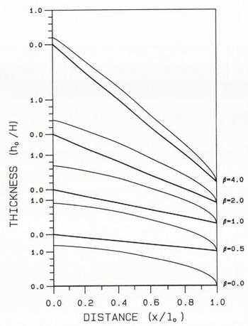
Fig. 10. Shape of steady–state glaciers for ε flow model (Equation (25)) with terminus sliding velocity ε = 0 and various bed slopes β.
Table III ε = 0, b1=0.01, variable b

From the preceding calculations, it appears that the size of the mass–balance perturbation and the maximum thickness of the glacier determine the volume perturbation. However, the effect of the spatial variation of b1 has not been addressed. On real glaciers, we may expect in some cases that b1 is far from spatially uniform (Reference BraithwaiteBraithwaite, 1980;Reference Reeh Reeh, 1983). The effects of spatial variation in b1 may be examined using the linearized theory. When flux per unit width q is linearized by Equation (5), the perturbed form of Equation (25) becomes
This equation can also be deduced by integration of the steady–state form of Equation (7). It has the unique regular solution

This expression can be integrated to yield the volume perturbation
By changing the order of integration and manipulating the resulting expression one finds
where
The function κ(x) represents the effect on V1 of a mass–balance perturbation concentrated at a point x on the glacier. Figure 11 shows the distribution of κ(x) evaluated using C0 and D0 for the model described by Equation (25) with β = 0 and ε = 0.05. κ(x) has a flat shape over most of the glacier, implying that the spatial variation of b1 is not important for the determination of V1 It is within 15% of its average value over nearly 90% of the length of the glacier. We conclude that it is the integrated mass–balance perturbation B 1 = l0〈b1〉 which determines the volume perturbation.
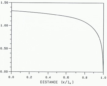
Fig. 11. Spatial weighting function x(x) for mass–balance distribution as defined by Equation (28).
Summary of results from time–independent modeling
The important results are:
-
(a) The volume perturbation V1 of a glacier, caused by a small mass–balance perturbation b1(x) is proportional to the integrated mass–balance perturbation, B 1 = l0〈b1〉, and is insensitive to the spatial distribution of b1.(x).
-
(b) The volume perturbation is not sensitive to the amount of sliding at the terminus.
-
(c) The volume perturbation increases proportional to the maximum thickness of the glacier.
-
(d) The effect of basal slope on the volume perturbation is limited to its effect on the maximum thickness.
In non–dimensional form, these results are embodied in the fact that V1/(h0 maxb1) ~ 1 independent of b1 ε, and β. When this is dimensionalized, the corresponding expression is V1/(h0 maxb1) ~ l0/b0 . Thus, the volume perturbation V1 and therefore the memory length TM of a glacier appear to be related in a simple way to the geometry of the datum glacier without any explicit dependence on the sliding velocity at the terminus. The next section explores this possibility.
VI. Geometrical Estimate Of The Memory Length Of A Glacier
The results from section V support the validity of a simplified geometrical analysis presented by Jóhannesson and others (1989). We summarize that analysis here. Figure 12 Fig. 12. Steady-state profiles calculated from the ε flow model (Equation (25)) for zero terminus sliding (t. = 0) and horizontal bed (β = 0) for b1 = 0 (solid — h0) and b1 = 0.1 (long-dashed — h∞ ). Short–dashed curve shows the profile for b1 = 0 shifted so its terminus coincides with the profile for b1 = 0.1. shows the initial steady–state profile h0 of a hypothetical (two–dimensional) glacier (full curve) and the final steady–state profile h∞ (long–dashed curve), after a small mass–balance perturbation b1. If b1 is sufficiently small, the two profiles will have essentially the same shape. The volume (per unit width) of the initial glacier and of the final glacier are then approximately given by V0 = gh0 maxl0 and V∞ = gh∞ max(l0 + l1 where is a geometrical factor which is the same for both cases because of the similarity of the profiles. Then
to first order in l1 and ∆hmax = h∞max — h0 max. Perfect plasticity theory for a glacier on a flat bed predicts hmax(1 − x/l)½ (Nye, 1951), which gives g = 2/3. This value of g is also fairly close to those values for any of the profiles found from Equations (26) or calculated numerically in this paper. We will take g = 2/3 as a representative estimate of g. Equation (12) gives the length change l1 as −l0〈b1〉/b0(l0). The change in maximum thickness may be estimated as ∆h max = (½)(l1/l0)h 0 max which tollows directly from the theoretical result h max ~ (l)½ found from either perfect plasticity theory (Nye, 1951) or the flux relationship (Equation (4b)) used here to find Equations (26). When these evaluations of g, l1 and ∆hmax are introduced into Equation (29), V1 . is found to be
This is the result found in section V, when one accounts for the fact b0(l0) is negative.
It is also possible to make a simple pictorial argument for Equation (30). Refer to Figure 12 and let the profile hQ be shifted to the right (short–dashed curve) so that the two termini coincide. Then the difference in the volume of the two profiles is to first approximation the shaded region to the left end of the figure. This volume is V1 = h 0 max l1 = −l0 〈b1〉h 0 max/b0(l0) which gives Equation (30) in a simple direct way. When this argument is applied to a glacier on a sloping bed or a valley glacier with zero thickness at the head, a cut is made through the glacier at the point of maximum thickness. The profile h 0 down–stream from the cut is shifted by l1 to the right as before, and it will then nearly coincide with h∞ . The cut opens by l1 = −l0 〈b1〉/b0(l0) and this again leads to Equation (30). This method was used by Johannsson (unpublished) to estimate the response time of the Grїmsvotn depression in Vatnajӧkull, Iceland, to a change in the geothermal heat flux which maintains the depression (Reference BjörnssonBjӧrnsson, 1974).
From the above discussion and Equation (30), we see that the change in the length of the glacier is the most important factor determining the volume change. This is related to our analysis (section V) of the effect that spatial variation in the balance rate b(x) exerts on the volume change. The response function к(х) in Equation (28a) has a flat shape over most of the glacier (Fig. 11). This means, to a first approximation, that it does not matter where a mass–balance change takes place on the glacier. We are now able to see this as a consequence of the fact that the change in length is a function of the integrated mass–balance perturbation, and does not depend on the spatial distribution of b1(x).
In order to relate Equation (30) to Equations (13) and (14) using the same picture, we may calculate 〈h1〉/h1(l0) by reference to the stippled area in Figure 12 (which of course is approximately equal to the shaded area). The shifted initial profile nearly coincides with the final profile, which means that h 1(x) = −l 1∂h 0/∂x. Integration of A1W over length then gives 〈h1〉 = l1h 0 max/l 0. Equations (11) and (12) give h1(l0) = −l1b0(l0)/u0(l0). This last result for h1(l0) is simply a statement that Bh0(10)ZBx, i.e. the slope of the terminus (A1(Z0VZ1) is the ratio of the ablation rate to the forward velocity and is consistent with the inverse relationship between slope of the terminus and terminus sliding velocity found in the numerical calculations in sections IV and V. The ratio <At> to b1(Z0) can be calculated from these two results to find ƒ = 〈h1〉/h1(l0) = −u0(l0)h 0 max/l0b0(l0) .The geometrical similarity then implies fis proportional to the sliding rate at the terminus. When this result is substituted into Equation (14b), Equation (30) is obtained.
It may seem unexpected that V1 depends only on h 0 max and An(Zn). The steady-state Ha, is reached when the geometry of the glacier has changed such that the How ol the glacier can support the additional flux required by the mass–balance perturbation. Then one might expect that some dynamical properties of the glacier would enter into the expression for V1 (for example, the parameters in the flow law). However, these are described by the initial profile A0. It is only necessary that the same dynamical properties determine the final profile, then it will be similar in shape. With regard to the terminus region, we do not need to know the details of the processes, but only that they remain the same as the glacier advances or retreats. It is therefore natural that the only variables determining the volume perturbation are the size of the initial profile and the relative size of the changes that occurred.
The volume perturbation given by Equation (30) is consistent with the conclusions (a) to (d) in section V, which were based on numerical modeling of Equations (3) and (4b). However, the above derivation of Equation (30) does not depend on the validity of Equations (3) and (4b). From the simplicity of the assumptions involved in the derivation of Equation (30), we may expect it to be valid even if some of the assumptions (for example, the neglect of longitudinal stress gradients) leading to Equations (3) and (4b) are unrealistic.
Equation (30) together with Equations (17a) and (21) lead to the estimate of the memory length TM of a glacier given by Equation (lb). Equation (lb) is not as fundamental as Equation (30), since it is based on additional assumptions inherent in Equations (19), (20), and (21). Nevertheless, the time–scale given by Equation (lb) is of fundamental importance for the adjustment of glaciers to climatic variations, since in any case it must represent a lower limit for the memory length.
VII. Discussion
In the introduction we pointed out that Equations (la) and (lb) seem to give very different estimates for the memory length Tm of a glacier. Both of these estimates of Tm arise from the recognition that Tm is equal to a volume time–scale TM = TV = V1II0 <At> (Equations (17a) and (21)).hey differ in the way the volume change V1 is obtained (Equation (14b)) in the case of Equation (la) and Equation(30) in the case of Equation (lb)). The appearance of disagreement therefore concerns disagreement about V1. For a given length change I1 and corresponding thickness change at the terminus A1(Z0), the question then hinges on how thickness change is spread up–glacier from the terminus. This is described by the geometrical factor f of Equation (13).
The flow models analyzed in sections IV and V, whether linearized or not, predict changes in thickness b1that are highly concentrated near the terminus. The factor f is small. In section V we showed that over most of the length of the model glaciers A1 is not sensitive to changes in terminus sliding velocity u(l0). The effect of u(l0) is localized near the terminus, and the value of f is approximately proportional to u(l0). When these values of f are used, Equations (la) and (lb) agree.
The identification of ƒ ~ ½ as a reasonable theoretical value for glaciers originated from an idealized model glacier invented by Nye (1963a, fig. 2) for illustrative calculations. It has been extensively reviewed by Reference PatersonPaterson (1981, chapter 12, p. 255–60) and Hutter (1983, chapter 6, p. 353–69). This model is described by distributions of kinematic wave velocity C0 and diffusion coefficient D0 as
with δ << 1 and 0 ≼ x ≼ l 0 = L(1 − δ). The parameter E controls the amount of diffusion; S is scaled to terminus sliding vleocity; L is a length scale; and σ is a time–scale. We refer to this model as the E,b model. Nye argued that these distributions of C0 and D0 are representative of distributions in real glaciers when S Footnote * IO−2, σ * 101 years, and E Footnote †1. The corresponding distributions of C0 and D0 are shown in Figure 8 for comparison with those associated with the ε model developed in sections IV and V. With E = 1 the thickness change A1 after a step change in mass balance approaches a linear variation between the glacier head and terminus, i.e. a triangular distribution that corresponds to / = iA (Nye, 1963a, fig. 3). The shape of the predicted A1 profile depends on the parameter E, but a nearly triangular distribution is maintained for values of E between 0.6 and 2, which includes the range of E expected to represent realistic diffusion. In physical terms, the thickness change at the terminus imposed by Equation (11) is spread long distances up–glacier by the effects of diffusion.
If the E,b model and the parameter values are actually representative of real glaciers, it would be reasonable to expect Ji to be a representative value of f. The corresponding memory lengths Tm predicted by Equation (la) would then be in the range of hundreds of years; this is the origin of the long time–scale that is commonly accepted as a valid theoretical prediction. However, we believe that the £,6 model is not appropriate for this purpose.
In the Appendix we show that the relationship between the change in volume V1 and terminus velocity U0(I0) predicted from kinematic wave theory is highly sensitive to the details of the distributions of C0 and D0, especially near the terminus. This difficulty arises in part because the terminus is a singular point of Equation (7), and Equation (11) is not a boundary condition in the usual sense. Rather, it arises from a regularity condition (Nye, 1963a, p. 437–40). By example, it is shown that if C0 and D0 are deduced from a flux relationship q = q(h,a), the steady–state profile Ap corresponding to q(h,a) and a datum mass–balance distribution A0 (in other words, if q(h,a), A0, C0, and D0 are internally consistent through Equations (4), (5), and (6)), then V1 and Tm are nearly independent of u0(l0). The linearization of our ε model examined in section IV has this consistency. The £,6 model is based on ad hoc independent assumptions about the distributions of C0 and D0 and lacks this consistency. That situation leads to a value of f in Equation (la) that is apparently independent of U0(I0), and leads to an unrealistic prediction of a 1/«0(Z0) dependence for V1 in Equation (14b) and the corresponding memory length τM. Other seemingly realistic distributions of C0 and Dg can give quite different dependencies of V1 and Tм on u0(l0).
Distributions of C0 and D0 derived for real glaciers from a realistic flux relationship may be internally consistent in the above sense. In this case, linearized kinematic wave theory will yield valid predictions, just as it does for our Ε model, when we use C0 and D0 derived from a datum steady state (see section IV). This is probably the reason why the response times of South Cascade Glacier, Washington, U.S.A., and Storglaciären, Kebnekaise, Sweden, predicted by kinematic wave theory (Nye, 1963b, 1965a, b), are not as long as would be expected by analogy with the £,6 model. One must bear in mind, however, that quite unrealistic predictions may result from inconsistencies in the derived distributions, especially near the terminus.
The analysis in this paper has been carried out with highly simplified geometry in comparison to reality. If a glacier advances or retreats over a terminal zone with large changes in bed slope (e.g. over cliffs) or bed structure (bed roughness or deformability), the assumption of longitudinal profile shape similarity could break down. Most glaciers have significant longitudinal variations of thickness. If these are large, for example with deep subglacial basins, the thickness h0max in Equation (30) must be replaced with a thickness scale based on an appropriate longitudinal average. Similarly diverging or converging flow caused by width variations exists on all glaciers and also in ice caps and ice sheets. Reference Jȯhannesson, Raymond and WaddingtonJohannesson and others (1989) have shown that Equation (30) would still hold, but in this case with only minor modification by a factor (A/V)dV /dA which describes how glacier volume is related to area. It is clear that Equation (30) and Equation (lb) are best regarded as approximate and useful for easy semi–quantitative estimates of the memory length of a glacier.
The long time–scale relationship between mass balance and terminus–position variations is difficult to examine directly on actual glaciers because existing time series of mass–balance data cover only a few decades. The analysis we have presented illuminates an alternative approach to the question of glacier memory through investigation of the geometry changes that glaciers have experienced, in particular the assumption about similarity of profile shapes and the geometrical factor f. Opportunities to test these ideas are provided by changes in glacier geometry from Neoglacial to present times. Repeated geodetic surveys of surface profiles extending over time intervals covering a significant fraction of the retreat from Neoglacial conditions have been made on some glaciers in the Alps and are especially valuable. Comparison of Neoglacial moraine crests and other morphological data with present ice surfaces could also be used in many mountain regions of the world.
VIII. Conclusions
Our theoretical conclusions reached in this paper are summarized as follows:
The interval of time TM over which a glacier responds to prior climate can in general be described by a volume time–scale TM.
Ihe volume time–scale TV can be computed from the volume differences between two steady–state profiles scaled to the causal mass–balance change.
Both Equations (la) and (Ib) are correct.
Correct evaluation of Equation (la) using kinematic wave theory involves difficult problems concerning details of behavior at the terminus.
Equation (lb) is a simpler estimate.
Commonly assumed memory lengths of 102–103 years for typical glaciers are not theoretically valid as a general rule.
Acknowledgements
This research was supported by U.S. National Science Foundation grant number EAR 8708391. Part of this research was carried out while T. Johannesson was employed at the Science Institute of the University of Iceland. We wish to thank J.F. Nye, R.LeB. Hooke, W.D. Harrison, and K..A. Echelmeyer for comments that helped us improve the manuscript.
Appendix
Three Linearized Glacier Models; Asymptotic Behaviour In The Limit Of Small Sliding At The Terminus
In the following we will use perturbation methods to analyze three different linear steady–state models of the form of Equation (7), with the time derivative omitted and with a uniform mass–balance perturbation bx(x) = 1. Of special interest is the volume perturbation
which determines the volume time–scale TV (Equation (17a)) and therefore the adjustment time TM of the model glacier (Equation (21)). The principal question concerns the asymptotic behaviour of V1 as sliding at the terminus goes to zero. Sliding at the terminus had little effect on the response of the numerical glacier models in section V. Equation (la), on the other hand, seems to predict that sliding at the terminus plays a key role in determining the response. Our goal is to explain in analytical terms the perhaps unexpected result of the numerical glacier models in section V.
Perturbation models (Reference ColeCole, 1968; Reference Kevorkian and ColeKevorkian and Cole, 1981) are often used to find approximate solutions to problems involving a small parameter 6. The solution of the problem is expanded as an asymptotic expansion in 6 (the “outer expansion”). Often this expansion fails to satisfy a boundary or a regularity condition. In that case, a different asymptotic expansion (the “inner expansion”) has to be used in a so–called boundary layer. In the following we will make frequent use of the “big O notation”, i.e. f(x) = 0(g(x)) as O(g(x)) as x → 0 means that the limit of (f/g) is finite as x → 0.
1. Nye’s (1963a) £,δ model
The model is described by the (non–dimensional) kinematic wave velocity C0 = x(l – x) and diffusion coefficient D0 = Ex2(1 − δ − x)
107] with 0 > δ >> 1 and 0 ≼ x ≼ l 0 = (1-δ) (see section VII for discussion). Integration of Equation (7) with respect to x (omitting the time derivative and putting b1(X) = 1) leads to the differential equation
for the steady–state change in thickness h1(X). By putting y = 1 − δ − x, this equation is more conveniently expressed as
There is no boundary condition, but the solution is required to be regular at the singular point y = 0 of the differential equation (Nye, 1963a, p. 437–40). Obviously, h
1(y = 0) = 1/δ. This suggests the expansion h
1 = ![]() . Substitution into Equation (Alb) and collection of terms with equal powers of & leads to differential equations for each of
. Substitution into Equation (Alb) and collection of terms with equal powers of & leads to differential equations for each of ![]() . The equation for
. The equation for ![]() is
is
Then
where k is a constant of integration. This solution is regular for all y, 0 ≼ x ≼ l 0 = (1 − δ).
This equation has a regular solution at у = 0 if K = 1.
Consequently, the constant of integration in h[°> can be determined from the equation for ![]() . Similarly, a constant of integration in can be determined by requiring that
. Similarly, a constant of integration in can be determined by requiring that ![]() be regular and in this way the expansion for h1 can be built up to any order without the introduction of a boundary layer. The lowest order, however, is sufficient for our purposes. It is given by
be regular and in this way the expansion for h1 can be built up to any order without the introduction of a boundary layer. The lowest order, however, is sufficient for our purposes. It is given by
Thus
This approximation is very good for small 8. For 6 as small as 0.006, as used by Nye (1963a), and E in the range 0.2 ≼ E ≼ 2.0, plots of h1(X) from Equation (A2) can hardly be distinguished by eye from plots of At(x) based on exact solutions of Equation (Ala). For very small £, the approximation fails since it is implicitly assumed in the preceding analysis that E = 0(1). For E = Ο(δ), a different scaling of the variables is necessary to produce a consistent approximation.
The volume perturbation V1 deduced from Equation (A2) is
The factor f = VJUnh1(I0)) in Equations (14) is evidently / = 1/(1 + )/E) + O(S) if E = 0(1).
The shape of A1 is essentially unaffected as δ → 0 and A1 is inversely proportional to 5 over almost the entire length of the glacier. V1 and therefore
Tv and тм go to infinity as S – 0. This means that the amount of sliding at the terminus determines the response of the whole glacier. It is difficult to imagine a physical process that can bring about this result. Therefore, we will now analyze a slightly different model in order to find out whether the 1/6 dependency of A1 and V1 only applies to this particular model or whether it is likely to be true in general for models of this kind.
2 A slightly modified £,6 model
The diffusion coefficient D0
must go to zero at the terminus (see section III for discussion). Thus, the steady–state form of Equation (7) will in general have a singular point at the terminus. This is indeed the case for the £,6 model which has a singular point at χ = I – 6. We may expect the steady–state solution to be sensitive to the form of O0, or more importantly to the form of the ratio D0/C0, as the singular point at the terminus is approached. Assuming q = q(h,a) and using the cyclic rule of partial derivatives, we can write ![]() −(∂h/∂α
q
. The partial derivative (∂h/∂α
q
expresses how small changes in A and α at a fixed location must be related to each other for the flux to remain constant at that location.
−(∂h/∂α
q
. The partial derivative (∂h/∂α
q
expresses how small changes in A and α at a fixed location must be related to each other for the flux to remain constant at that location.
In the interior of the glacier, outside a zone near the terminus where special considerations must apply, we expect a flux relationship of the form of Equation (4b) to be valid. A flux relationship of this form predicts that
D0ZC0 = –(QhZQa)cl =
(rZs)h0Za0. Since A0 decreases towards the terminus and O0 probably increases, D0 must decrease faster than C0 as the terminus zone is approached. This may be crudely quantified for a glacier on a flat bed by assuming that A0 decreases as some power of the distance from the terminus U — X (a square–root shape is commonly assumed to be realistic). Then D0ZC0 = (r/.s)h0/ (–dA0/dx) = O(l0 – x). We see that in this case the ratio D0ZC0 will decrease proportional to I0 – x. The distributions of D0 and C0 for the ε model presented in this paper (Fig. 8) clearly show this behavior. So do published calculations of D0 and C0 based on real glacier profiles (e.g. Nye, 1965b, fig. 5;Reference Reeh Reeh, 1983, p. 38–53; however, figure 7 in Nye (1963b) does not show this as well).
The above argument does not apply to the terminus zone, where a flux relationship of the form of Equation (4b) breaks down. However, it turns out to be crucial that the form of C0 and D0 is realistically modeled outside the terminus zone where we assume a flux relationship of this form to be valid.
Both D0 and C0 in Equation (Ala) decrease linearly as x → l0 . Based on the above discussion, this is not realistic and we replace D0 = Ex2(1 − δ − x) in Equation (Ala) with D0 = Ex(1 − δ − x)2 in order to investigate the effect of the shape of D0 near the terminus on the solution. In addition to replacing (1 − δ − x) with (1 − δ − x)2 to produce the required ratio of D0ZC0 near the terminus, we have also replaced x2 with Y This is done in order to simplify the analysis and does not change the nature of the problem. With this modification, Equation (Ala) becomes
or defining as before y = 1 − δ − x
] One quickly finds that the method used for Equation (Alb) does not work here. It is not possible to derive an outer expansion which is regular at у = 0. This indicates the occurrence of a boundary layer at the terminus.
A differential equation for the boundary layer is deduced by re–scaling both the dependent and the independent variables. In this case, the correct scaling is given by y* = y/δ, ![]() , which leads to
, which leads to
We see that the small parameter 6 has been scaled out of the problem. This is not unusual for perturbation problems and means that at least in the boundary layer the full equation has to be solved. The unique regular solution of Equation (A5) is readily found to be
From this solution, both the nature of the boundary layer and the asymptotic behavior of the solution in the interior of the glacier can be derived.
The boundary layer is of width 0(6) and within it the solution is
0(1/8). Its contribution to V1 is therefore O(l).
Away from the boundary layer, the asymptotic behavior of A1O) as 6 – O depends on the behavior of ![]() y/δ → ∞ for a fixed value of y. Depending on the numerical value of E, we find that as y
* → ∞
y/δ → ∞ for a fixed value of y. Depending on the numerical value of E, we find that as y
* → ∞
where Γ is the gamma function,  .
.
Then ![]() is given by
is given by
as δ → 0 for a fixed y, in the interior of the glacier outside the boundary layer at the terminus.
The contribution to V– from Zi1 outside the boundary layer can be found by integrating A1O–) in the interior of the glacier (Equation (A6)). This is the most important contribution to V1 and we can derive the following order–of–magnitude estimate
The factor ƒ = V1/(l0h1(l0)) in Equations (14) goes to zero as 6 –* 0. This arises because the thickness change is only partially spread up–glacier from the terminus where h1(Z0) = 1/8. For E in the range 0 E 1, Zi1 is even independent of 8 outside the boundary layer at the terminus. This is similar to what we found for the Ε model in section V (Fig. 9).
Equation (A7) predicts that V1 and therefore
TV and TM go to infinity as δ → 0 as was the case for the £,8 model. The dependency of It1 and V1 on 8 as 8 – 0 is, however, quite different from the £,8 model and this indicates that analytical models of this kind are highly sensitive to the details of the distributions of D0 and C0, especially near the terminus. Therefore, it must be crucial that the distributions of D0 and C0 are realistic in models of this kind. Otherwise, almost any result may be obtained. In particular, the prediction of the £,5 model that the volume change V1 is inversely proportional to sliding at the terminus, cannot be regarded as a valid theoretical prediction for real glaciers, since other seemingly more realistic distributions of D0 and C0 yield quite different predictions.
3. A model derived from a steady–state profile
In numerical models of glacier flow, the terminus has traditionally been treated in a very crude way (e.g.Reference Budd and Jenssen Budd and Jenssen, 1975;Reference Bindschadler Bindschadler, 1982;Reference Waddington Waddington, unpublished). The grid size of the models is usually so coarse that detailed modeling of the terminus is out of the question. Instead, it is assumed that the terminus plays no active role in the dynamics of the glacier as a whole. The position of the terminus is determined from simple continuity requirements, i.e. the shape of the terminus is assumed constant and the rate of change of its position is determined by the ice flow past the last grid node up–stream from the terminus. These models cannot produce any effect of the terminus on the glacier dynamics, since the expected passive behavior of the terminus is built into the models as an assumption.
The assumption of a passive terminus is a physically appealing one. One would expect realistic analytical models to have a similar property, even if it is not included at the outset as an assumption. In this view, the crucial part of the model is the correct specification of the model parameters (i.e. D0 and C0) in the interior of the glacier, where the proposed flux relationship is assumed valid. The region very close to the terminus, where the flux relationship breaks down, must be included in the model in some way, but from physical grounds one would expect this region to be isolated from the rest of the model. Mathematically, this could for example arise if an isolated boundary layer is located at the terminus. Needless to say, the behavior of V1 in the limit of zero sliding at the terminus must be non–singular. Otherwise, the terminus region determines the response of the whole glacier.
We will now derive a simple glacier model based on the flux relationship expressed by Equation (4b) and investigate whether consistent specification of D0 and C0 leads to the results discussed above. Both D0 and C0 are defined as partial derivatives of the same quantity (Equations (6)). Therefore, they cannot be specified independently, but must be based on a specific flux relationship, datum mass balance, and the corresponding steady–state profile. We will investigate a two–dimensional ice sheet on a flat bed and take K – 1, г = 3, and s = 5 in the flux relationship (Equation (4b)). h0 in the ablation area is then given by
when A0 is uniform A0(x) = –1 in the ablation area (Reference Paterson and ColbeckPaterson, 1980). The corresponding D0 and C0 (Equations (6)) are
where we have added the term 6 in the expression for C0in order to provide a non–zero C0 at the terminus χ = Z0–
We see that D0 decreases faster than C0 as χ – /0 as expected.
Adding 6 to C0 is admittedly an arbitrary way of specifying the terminus dynamics. As discussed above, it is the consistency of A0, D0, and C0 in the interior of the glacier which is of primary concern. Given consistency, the details of the terminus dynamics should not be important for the dynamics of the glacier as a whole. Therefore, this ad hoc way of specifying the terminus dynamics is adequate for our purpose.
In the accumulation area, the expression for A0 is different from Equation (A8) and consequently the corresponding expressions for D0 and C0 are different from Equations (A9). Arithmetic simplicity makes it worthwhile to analyze the ablation area without considering the accumulation area. This can be done if it is assumed that that mass–balance perturbation A1(Jt) is confined to the ablation area, since then the thickness change A1(Ac) in the ablation area will be independent of the accumulation area. Assuming an ablation area extending from x = 0 to x = 1 with a uniform mass–balance perturbation b1(X) = 1, this model is expressed by the following equation
with D0 and C0 expressed by Equations (A9). The accumulation area is located to the left of χ = 0 and is not considered.
After a change of variables to y = l0 − x = 1 − x for convenience, the outer expansion to lowest order satisfies the equation
The solution of this equation is
This solution is singular at у = 0 for any value of the integration constant K. Therefore, a boundary layer at у = 0 is needed. The integration constant K must be determined by matching to the boundary layer (Reference Kevorkian and ColeKevorkian and Cole, 1981, p. 24).
The boundary–layer equation is deduced by re–scaling у and A1. The correct scaling is ![]() . Using Equations (A9), Equation (AlO) transforms to
. Using Equations (A9), Equation (AlO) transforms to
and the equation determining the lowest–order term A1’0’, in the inner expansion is
This equation has the unique non–singular solution.
In very simple terms, matching of Equations (All) and (A 12) is done by requiring that, when expressed in the same variables, the equations agree to highest order “outsidejust outside” the boundary layer. When y * → ∞ (by letting 8–0 for a fixed y), the lowest–order term in the boundary layer (Equation (A 12)) becomes
Expressed in outer variables, this expression for the boundary layer becomes
as δ → 0 for a fixed у. This means that we must have K = O if the boundary layer (Equation (A 12)) is to merge smoothly with the outer solution (Equation (All)). Thus,
The boundary layer (Equation (A12)) is of width O(δ2) and within it the solution is O(1/δ). Its contribution to V1 is therefore 0(6) and goes to zero as 6–0. The outer solution (Equation (A 13)) can be integrated without difficulty to find V 1
which is finite in the limit 6 = 0. the factor f =
V1/(l0h1(l0) in Equations (14) is O(δ) as δ → 0.
Equation (A13) shows that, away from the terminus, A1 is determined by the dynamics in the interior of the glacier and independent of the amount of sliding at the terminus. Equation (A 14) shows that V1 and therefore rv and
TM are also determined by the dynamics in the interior of the glacier, and finite in the limit 8–0. This is what we expected to find for an analytical model with consistent specification of A0, D0, and
C0. We expect other models with carefully specified
D0 and Cn (for example, based on a flux relationship expressed by Equation (4b) with other values of r and s than used here, or models with different formulation of C0 near the terminus), to exhibit the same properties as the model presented here. In section VI, we found that geometrical similarity of steady–state glacier profiles leads to the conclusion that f is proportional to the sliding rate at the terminus. This is the case here since f = 0(8). Therefore, the ratio ƒ/u(l) = ƒ/δ in Equation (la) is approximately constant for small 8, and Equation (la) is consistent with Equation (lb). This model agrees with the numerical results of the paper, which are derived from a more complete formulation, which does not permit an analytical analysis.
We conclude that consistent specification of A0, O0, and C0, based on a specific flux relationship and datum mass balance, is essential for successful analytical models.


