


1. Introduction
Understanding the flow dynamics across nanometric channels plays an important role in the development of biomedical and chemical technology, from biosensors for cancer detection (Díaz-Cervantes, Robles & Aguilera-Granja Reference Díaz-Cervantes, Robles and Aguilera-Granja2018; Stirling Reference Stirling2018; Zhiani, Razavipanah & Emrani Reference Zhiani, Razavipanah and Emrani2018) to ultrafast filtration membranes (Chu et al. Reference Chu, Chin, Huen and Ferrari1999; Majumder et al. Reference Majumder, Chopra, Andrews and Hinds2005a; Whitby & Quirke Reference Whitby and Quirke2007; Joseph & Aluru Reference Joseph and Aluru2008; Davey & Schäfer Reference Davey and Schäfer2009; Sears et al. Reference Sears, Dumée, Schütz, She, Huynh, Hawkins, Duke and Gray2010; Das et al. Reference Das, Ali, Hamid, Ramakrishna and Chowdhury2014).
Most of the current applications of nanofluidic devices mimic biological channels by synthesizing nanostructures of similar size and geometry (Walczak et al. Reference Walczak, Boiarski, Cohen, West, Melnik, Shapiro, Sharma and Ferrari2005; Fang et al. Reference Fang, Wan, Gong, Lu and Li2008; Hou, Guo & Jiang Reference Hou, Guo and Jiang2011). As a consequence, large efforts have been made to expand the spectrum of nanostructures capable of conveying fluid flow. Nowadays, nanofluidic systems span a diversity of materials and arrangements of channels whose size ranges from a few nanometres to tenths of micrometres, both in cross-sectional area and length (Martin et al. Reference Martin, Walczak, Boiarski, Cohen, West, Cosentino and Ferrari2005).
A complete picture of the physical and chemical properties of the fluid/confining medium system is fundamental in order to design and simulate nano-devices, carry out experiments and, subsequently, implement nanofluidic technology for target applications. As the confinement size is reduced, the surface-to-volume ratio increases, and the fluid/confining medium interactions turn out to be fundamental to the dynamics of fluid flow at nanoscales.
The magnitude of the fluid/confining medium interaction along with the wall's rugosity play a role in the permeability of fluids confined within nanostructures. Particularly, the weak interaction and low rugosity between water and carbon nanotubes has been shown to be responsible for the low-friction flow observed in experiments with membranes (Hummer, Rasaiah & Noworyta Reference Hummer, Rasaiah and Noworyta2001; Majumder et al. Reference Majumder, Chopra, Andrews and Hinds2005a; Whitby & Quirke Reference Whitby and Quirke2007; Joseph & Aluru Reference Joseph and Aluru2008; Bonthuis et al. Reference Bonthuis, Rinne, Falk, Kaplan, Horinek, Berker, Bocquet and Netz2011). Understanding the tube/fluid interaction has allowed modification of the friction at the tube/fluid interface by chemical functionalization of carbon nanotubes (Majumder, Chopra & Hinds Reference Majumder, Chopra and Hinds2005b; Kim et al. Reference Kim, Chen, Johnson and Marand2007; Qiu et al. Reference Qiu, Wu, Pan, Zhang, Chen and Gao2009; Chan et al. Reference Chan, Chen, Surapathi, Taylor, Shao, Marand and Johnson2013; Feng et al. Reference Feng, Xiong, Wang, Cui, Sun and Wang2018; Wei & Luo Reference Wei and Luo2018). Also, flow permeability is sensitive to changes in tube rugosity, as observed in several types of nanopipes and nanochannels (Kyotani, Tsai & Tomita Reference Kyotani, Tsai and Tomita1996; Rossi et al. Reference Rossi, Ye, Gogotsi, Babu, Ndungu and Bradley2004; Miller, Young & Martin Reference Miller, Young and Martin2001; Mattia et al. Reference Mattia, Rossi, Kim, Korneva, Bau and Gogotsi2006b; Mattia, Bau & Gogotsi Reference Mattia, Bau and Gogotsi2006a; Whitby & Quirke Reference Whitby and Quirke2007; Whitby et al. Reference Whitby, Cagnon, Thanou and Quirke2008; Cao et al. Reference Cao, Huang, Ma, Lu and Lu2018). However, tuning the permeability of the confined fluid is possible only to some extent, since the capability to functionalize the tube surface and modify its rugosity is limited (Yang et al. Reference Yang, Li, Jiang, Du, Zhao and Zhao2010b; Wu et al. Reference Wu, Chen, Li, Li, Xu and Dong2017). Novel strategies to push such limits are developed continuously.
Despite all the advances achieved so far, there are some aspects of the physics of nanofluidic systems that have not been addressed in full detail. This is a challenge for flow control and has limited, to some extent, the implementation of potential applications of nanofluidic devices (Holt et al. Reference Holt, Park, Wang, Stadermann, Artyukhin, Grigoropoulos, Noy and Bakajin2006; Kannam et al. Reference Kannam, Todd, Hansen and Daivis2013; Ritos et al. Reference Ritos, Mattia, Calabrò and Reese2014; Wu et al. Reference Wu, Chen, Li, Li, Xu and Dong2017). In particular, it is necessary to go deeper into the description of the fluid/confining medium interactions in dynamic situations where a sustained motion is exerted on the confining media, either by thermal fluctuations or by other types of external forces (Krishnan et al. Reference Krishnan, Dujardin, Ebbesen, Yianilos and Treacy1998).
Most of the theoretical studies done to explain and predict the efficiency of nanofluidic devices have been done using molecular dynamics (MD) and continuum mechanics (CM). Both approaches have been useful under different approximations and physical situations. MD is especially useful to account for tubes of small radii, where the continuum description is not suitable and a complete description must account for the low-density regime in which fluid particles collide with the tube walls (Thomas & McGaughey Reference Thomas and McGaughey2009). However, the simulation of long tubes and long sampling times is not attainable with MD due to the computational expense demanded. Moreover, a realistic description of the interaction between tube and fluid is not clearly established in the literature; in particular, the nature of the interaction forces between water molecules and graphene-like structures has been shown to be strongly dependent on the value of the parameters used in the different force fields in the literature (Hummer et al. Reference Hummer, Rasaiah and Noworyta2001; Werder et al. Reference Werder, Walther, Jaffe, Halicioglu and Koumoutsakos2003; Holt et al. Reference Holt, Park, Wang, Stadermann, Artyukhin, Grigoropoulos, Noy and Bakajin2006; Joseph & Aluru Reference Joseph and Aluru2008; Bonthuis et al. Reference Bonthuis, Rinne, Falk, Kaplan, Horinek, Berker, Bocquet and Netz2011; Kannam et al. Reference Kannam, Todd, Hansen and Daivis2013; Wu et al. Reference Wu, Chen, Li, Li, Xu and Dong2017; Wei & Luo Reference Wei and Luo2018). The choice of an appropriate force field is always dependent on the type of property desired to be simulated computationally and on the experimental arrangement that one intends to reproduce (Werder et al. Reference Werder, Walther, Jaffe, Halicioglu and Koumoutsakos2003; Alexiadis & Kassinos Reference Alexiadis and Kassinos2008; Nakamura & Ohno Reference Nakamura and Ohno2012), rather than on the accurate description of the chemical interaction. This limitation is intrinsic to all MD simulations.
In contrast, CM has allowed for the simulation of relatively large tubes at any time scale, but at the cost of losing details in the description of flow properties that depend on the formation of complex molecular aggregates or structures (Yoon, Ru & Mioduchowski Reference Yoon, Ru and Mioduchowski2005; Whitby & Quirke Reference Whitby and Quirke2007; Wang & Ni Reference Wang and Ni2008; Zhen & Fang Reference Zhen and Fang2010; Arash & Wang Reference Arash and Wang2012; Gărăjeu, Gouin & Saccomandi Reference Gărăjeu, Gouin and Saccomandi2013; Kelly, Balhoff & Torres-Verdín Reference Kelly, Balhoff and Torres-Verdín2015). Efforts to account for both levels of physical description have inspired the development of hybrid approaches (Werder, Walther & Koumoutsakos Reference Werder, Walther and Koumoutsakos2005; Mohamed & Mohamad Reference Mohamed and Mohamad2010; Alexiadis et al. Reference Alexiadis, Lockerby, Borg and Reese2013; Ritos et al. Reference Ritos, Borg, Lockerby, Emerson and Reese2015). However, studies of fluid/confining medium systems at nanoscales in hybrid frameworks are also dependent on the force field parameters used, the chemical compositions of tube and fluid and on the implementation details of the simulation. Moreover, the comprehension of the underlying physical principles is a challenge in MD and hybrid frameworks, since there is no simple procedure to establish general trends or simplified expressions from the large number of simulated chemical systems in the literature that generalize the behaviour of carbon nanotubes conveying flow. In contrast, the CM approach allows for modelling of the complex fluid/tube interaction in an understandable manner, via a mean description of the interaction. In the literature, CM studies of nanostructures conveying fluid have considered static rigid tubes in which the fluid/tube interaction has been incorporated by the slippage of the fluid at the fluid–solid interface (Majumder et al. Reference Majumder, Chopra, Andrews and Hinds2005a; Whitby & Quirke Reference Whitby and Quirke2007). However, there is no agreement in the magnitude of slip length in carbon nanotubes conveying flow, since this description inherits the limited knowledge existing on the tube/fluid interaction (Bonthuis et al. Reference Bonthuis, Rinne, Falk, Kaplan, Horinek, Berker, Bocquet and Netz2011; Kannam et al. Reference Kannam, Todd, Hansen and Daivis2013; Ritos et al. Reference Ritos, Mattia, Calabrò and Reese2014; Li et al. Reference Li, Wang, Pan and Zhao2016; Wu et al. Reference Wu, Chen, Li, Li, Xu and Dong2017).
Numerous techniques and materials have been developed for the preparation of nanostructures for fluid transport, such as solid-state pores (Storm et al. Reference Storm, Chen, Ling, Zandbergen and Dekker2003; Dekker Reference Dekker2007; Yameen et al. Reference Yameen, Ali, Neumann, Ensinger, Knoll and Azzaroni2009; Li et al. Reference Li, Fustin, Lefèvre, Gohy, De Feyter, De Baerdemaeker, Egger and Vankelecom2010; Yusko et al. Reference Yusko, Johnson, Majd, Prangkio, Rollings, Li, Yang and Mayer2011), nanochannels (Walczak et al. Reference Walczak, Boiarski, Cohen, West, Melnik, Shapiro, Sharma and Ferrari2005; Camargo, Satyanarayana & Wypych Reference Camargo, Satyanarayana and Wypych2009; Yang et al. Reference Yang, Yang, Kim, Jeon, Oh, Choi, Hahn and Kim2010a; Hou et al. Reference Hou, Guo and Jiang2011; Kortaberria & Tercjak Reference Kortaberria and Tercjak2016; Rahman Reference Rahman2018), nanotubes (Majumder et al. Reference Majumder, Chopra, Andrews and Hinds2005a; Joseph & Aluru Reference Joseph and Aluru2008; Qin et al. Reference Qin, Yuan, Zhao, Xie and Liu2011), nanopipes (Kyotani et al. Reference Kyotani, Tsai and Tomita1996; Miller et al. Reference Miller, Young and Martin2001; Rossi et al. Reference Rossi, Ye, Gogotsi, Babu, Ndungu and Bradley2004; Mattia et al. Reference Mattia, Bau and Gogotsi2006a,Reference Mattia, Rossi, Kim, Korneva, Bau and Gogotsib; Whitby & Quirke Reference Whitby and Quirke2007; Whitby et al. Reference Whitby, Cagnon, Thanou and Quirke2008) and protein-based nanopores (Alcaraz et al. Reference Alcaraz, Ramírez, García-Giménez, Lopez, Andrio and Aguilella2006; Jung, Bayley & Movileanu Reference Jung, Bayley and Movileanu2006; De La Rica & Matsui Reference De La Rica and Matsui2010). Most of these nanostructures share one property: they have an elastic response to small mechanical deformations (Lu Reference Lu1997; Ruoff, Qian & Liu Reference Ruoff, Qian and Liu2003; Ji & Gao Reference Ji and Gao2004; Guo & Zhao Reference Guo and Zhao2007; Feng et al. Reference Feng, Xia, Li and Li2009).
The different types of deformation exerted on nanotubes allow for several strategies of mechanical manipulation. The role of the radial expansion and compression has been studied and compared with previously known results in micro and macrofluidic devices (Zhao et al. Reference Zhao, Ando, Qin, Kataura, Maniwa and Saito2002; Machón et al. Reference Machón, Reich, Telg, Maultzsch, Ordejón and Thomsen2005; Araujo et al. Reference Araujo2008). However, the role of size in the dynamics of elastic nanotubes is particularly important in a very specific type of elastic deformation: flexural bending. At nanoscales, flexural bending has two interesting and useful qualities: it requires a very small external force to cause it, from several pN to some nN – which is considerably smaller than the forces involved in radial expansion or compression (Salvetat et al. Reference Salvetat, Bonard, Thomson, Kulik, Forro, Benoit and Zuppiroli1999) – and it has a high-frequency response to those external forces, in the range of kHz to GHz (Krishnan et al. Reference Krishnan, Dujardin, Ebbesen, Yianilos and Treacy1998; Lourie & Wagner Reference Lourie and Wagner1998; Poncharal et al. Reference Poncharal, Wang, Ugarte and De Heer1999; Gibson, Ayorinde & Wen Reference Gibson, Ayorinde and Wen2007). In terms of energy, the bending of nanotubes can be produced in the range of  $[1\text {--}1000]\ \textrm {kT}$, where k stands for the Boltzmann constant and $T$ is temperature, depending on the tube length and radius. This means that bending modes might be excitable at room temperature, particularly for large length-to-radius ratios.
The capability to generate high-frequency vibrations by mechanical manipulation at a very small energetic cost opens up a landscape of possibilities that deserves further exploration, since it could be of potential use to improve both knowledge and control of the fluid dynamics at nanoscales. Some efforts have been made in such direction. Previous theoretical CM studies have demonstrated the relationship between the magnitude of fluid flow conveyed within an oscillating nanotube and the frequency of tube deflection (Yoon et al. Reference Yoon, Ru and Mioduchowski2005; Wang & Ni Reference Wang and Ni2008; Zhen & Fang Reference Zhen and Fang2010; Liu et al. Reference Liu, Liu, Dai and Cheng2018). Recently, the experimental feasibility of flow determination by measurement of the tube oscillation frequency by taking advantage of such a relationship has been theoretically proposed (Torres-Herrera & Corvera Poiré Reference Torres-Herrera and Corvera Poiré2018). In such studies, incorporation of tube vibrations in the description of nanoscale flow has been addressed by a model that is focused on the dynamics of a tube conveying a plug flow, i.e. flow velocity is a constant parameter of the model.
A CM model that fully couples the tube and fluid dynamics, accounting for external driving forces, velocity profile and axial dependence of flow velocity, is missing in the literature. We consider that a model with these features can be derived by means of simple physical and geometrical constraints, via a formulation based on the principle of least action (Djukic & Vujanovic Reference Djukic and Vujanovic1971; Lebon & Lambermont Reference Lebon and Lambermont1973; Leech Reference Leech1977; Bedford & Drumheller Reference Bedford and Drumheller1983; Salmon Reference Salmon1983; Bedford Reference Bedford1985; Sieniutycz & Berry Reference Sieniutycz and Berry1989; Shepherd Reference Shepherd1990; Benaroya & Wei Reference Benaroya and Wei2000). This approach has been useful to study complex geometries, such as the flow dynamics inside compressible nanobubbles (Teshukov & Gavrilyuk Reference Teshukov and Gavrilyuk2002) and systems subject to very complicated physical interactions, such as magnetorheological fluids (Sun, Zhou & Zhang Reference Sun, Zhou and Zhang2003).
In this work, we derive a system of two coupled equations of motion for the dynamics of a fluid and a confining nanotube, when this one is subject to periodic bending deflections. In order to do so, a theoretical treatment based on the principle of least action allows us to account for the complex fluid/tube interaction in a simple understandable manner, that couples the tube and fluid dynamics via a constraint in the flow velocity. Our formulation allows for a broad comprehension of when the dynamics of the fluid affects the tube, of when the dynamics of the tube affects the fluid, in which case the dynamics is fully decoupled, and for which situations the fully coupled equations should be solved. Such a panorama could not be attained with the numerical schemes reported in the literature for nanotubes conveying fluid subject to oscillations (Wang & Ni Reference Wang and Ni2008). As an example of the different phenomena that our methodology allows us to reveal, we report a new phenomenon in the limit at which the tube modifies the dynamics of the fluid, i.e. it gives a modified linearized Navier–Stokes equation, accounting for the tube effect on the fluid motion. We predict an oscillating velocity for the fluid within the nanotube, with twice the frequency of the latter one, that persists at high frequencies, even for a fluid driven by a constant pressure drop.
2. Methodology
Our approach is based on the minimal action principle, which has successfully been used to establish the Navier–Stokes dynamics when a fluid is subject to a wide range of forces and restrictions (Djukic & Vujanovic Reference Djukic and Vujanovic1971; Lebon & Lambermont Reference Lebon and Lambermont1973; Leech Reference Leech1977; Salmon Reference Salmon1983; Bedford Reference Bedford1985; Sieniutycz & Berry Reference Sieniutycz and Berry1989; Shepherd Reference Shepherd1990; Benaroya & Wei Reference Benaroya and Wei2000). Such a methodology is particularly useful when constraints are imposed on a physical system, since it is capable of accounting for the restrictions in the resulting equation of motion in a straightforward and consistent manner (Bedford & Drumheller Reference Bedford and Drumheller1983; Bedford Reference Bedford1985; Teshukov & Gavrilyuk Reference Teshukov and Gavrilyuk2002).
We model a tube/fluid system via two dynamic variables: the vertical tube position,  $u$, and the flow velocity, $v$. In order to do so, we consider that the tube is an Euler–Bernoulli elastic cylindrical shell subject to small deformations and no axial tension. Also, the tube radius is much smaller than the curvature radius of the tube at its maximum deflection. Besides, we consider a Newtonian incompressible fluid. The system is kept at constant temperature, which implies a constant fluid viscosity and also allows us to study the fluid dynamics without considering equations for heat transfer processes.
2.1. Principle of least action
Two frames of reference arise in the study of a fluid confined within an oscillating tube: a static frame,  $(x,y,z)$, which is an inertial frame of reference and is used to describe the tube motion; and a dynamic frame, which is a non-inertial frame and is used to describe the fluid motion, which consists of cylindrical coordinates $(r',\theta ',z')$ or equivalently, $(x',y',z')$ such that the
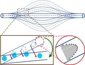
  $z'$-axis is located at the centre of the tube as it moves. A scheme of the physical system and the frames of reference is shown in figure 1. The relation between the static and dynamic frames of reference is given in appendix B.

Figure 1. Description of the model. The system consists of an elastic tube, described by its vertical displacement  $u(z,t)$, conveying a fluid described by the axial flow $v(r',\theta ',z',t)$, according to a local cylindrical frame of reference, whose origin is located in the tube symmetry axis. The $z$ axis coincides with the tube symmetry axis when the tube is undeformed.
The principle of least action for this system is given by
 \begin{equation} \delta S+\delta W+\delta C = 0 , \end{equation}
where  $S$ is the action of the system, $W$ accounts for the external and the non-conservative work applied on the system and $C$ accounts for the constraints; $\delta S$, $\delta W$ and $\delta C$ are the corresponding variations of these quantities. The action, $S$, is given in terms of the Lagrangian, $L$, which is the difference between the kinetic and potential energy of the system, as
 \begin{align} S & = \int_{t}L\,\textrm{d}t \nonumber\\ & = \int_{t}(T_{t}+T_{f}-V_{t}-V_{f}-V_{t/f})\,\textrm{d}t , \end{align}
where  $V_{t/f}$ denotes the interaction potential between tube and fluid, whereas the kinetic and potential energies of the tube and the fluid are denoted by $T_{t}$, $T_{f}$, $V_{t}$ and $V_{f}$, respectively, and are given in terms of the vertical displacement of the tube, $u(z,t)$, and the fluid velocity vector, $\boldsymbol {v}_{\boldsymbol {fluid}}(\boldsymbol {r},t)$. The study can be applied to any elastic hollowed nanostructure, regardless of the specific geometry of its cross-section. For this particular derivation, a cylindrical tube is considered.
With these considerations, each term in (2.2) is expressed as
 \begin{gather} T_{t}=\int_{V}\tfrac{1}{2}\rho_{t} \left|\boldsymbol{v}_{\boldsymbol{tube}}\right|^{2}\,\textrm{d}V , \end{gather}
 \begin{gather}T_{f}=\int_{V}\tfrac{1}{2}\rho \left|\boldsymbol{v}_{{\boldsymbol{fluid}}}\right|^{2}\,\textrm{d}V , \end{gather}
 \begin{gather}V_{t}=\int_{V}\frac{1}{2}\rho_{t}e_{t}\left(\frac{\partial u}{\partial z},\frac{\partial^{2} u}{\partial z^{2}}\right)\textrm{d}V \quad \mbox{and} \end{gather}
 \begin{gather}V_{f}=\int_{V}\rho e\left(\rho,\frac{\partial \boldsymbol{r}_{{\boldsymbol{fluid}}}}{\partial x'},\frac{\partial \boldsymbol{r}_{\boldsymbol{fluid}}}{\partial y'},\frac{\partial \boldsymbol{r}_{{\boldsymbol{fluid}}}}{\partial z'}\right)\textrm{d}V , \end{gather}
while  $V_{t/f}$ depends on the force field employed and on the level of physical detail of the model. As we will show later, we take advantage of the principle of least action to model the tube/fluid interaction via a geometrical constraint, and therefore we consider $V_{t/f}=\text {const}$. The potential energy of the tube is given by the bending energy of an Euler–Bernoulli cylindrical shell, which is a widely used model to study the properties of a bent tube (Chen Reference Chen1985; Gibson et al. Reference Gibson, Ayorinde and Wen2007; Wang & Ni Reference Wang and Ni2008; Bauchau & Craig Reference Bauchau and Craig2009). Axial tension caused by changes in tube length is negligible for tubes subject to small amplitude deformations; besides, nanotubes in typical experimental settings are not subject to external axial tensions, so we consider no axial tension. In this case, the Euler–Bernoulli potential energy for an elastic shell with Young's modulus $E$ leads to the following expression:
 \begin{equation} V_{t}=\int_{V}\frac{1}{2}y^{2}E \left(\frac{\partial^{2} u}{\partial z^{2}}\right)^{2}\,\textrm{d}V . \end{equation}
 The potential energy of the fluid arises from the interaction between its particles. In a CM approach, the interaction potential between particles responds to changes in the bulk density,  $\rho$, and the strain, $\partial \boldsymbol {r}_{{\boldsymbol {fluid}}}/\partial x_{i}$. For this reason, the potential energy in (2.6) is given in terms of a local potential energy per unit mass, $e$, that depends on those quantities. Hence, the potential energy of incompressible fluids with no elastic properties is considered as a constant (Bedford Reference Bedford1985).
The pressure and the viscosity of the fluid are considered through the term  $W$ in (2.1). The viscous forces are excluded of the potential energy because they are dissipative. From a mathematical point of view, dissipative forces have a functional dependence on fluid velocity and its spatial derivatives, rather than on fluid displacement. For an incompressible fluid that moves along the $z'$-direction subject to a stress given by pressure $p$ and the viscous shear stress ${\boldsymbol {\tau }}$, the variation of $W$ is given by
 \begin{equation} \delta W = \int_{t}\int_{S}\boldsymbol{F}_{\boldsymbol{ext}}\boldsymbol{\cdot} \delta\boldsymbol{r}_{{\boldsymbol{fluid}}}\,\textrm{d}S\,\textrm{d}t = \int_{t}\int_{S}({-}p\boldsymbol{\mathsf{1}}+{\boldsymbol{\tau}})\boldsymbol{\cdot}\boldsymbol{n} \boldsymbol{\cdot}\delta \boldsymbol{r}_{{\boldsymbol{fluid}}}\,\textrm{d}S\,\textrm{d}t, \end{equation}
where  $\boldsymbol {n}$ denotes the vector normal to the surface at which the force is exerted. It is important to point out that Hamilton's principle allows us to incorporate a force in multiple manners which are mathematically equivalent (Bedford Reference Bedford1985; Goldstein, Poole & Safko Reference Goldstein, Poole and Safko2002), leading to the same equations of motion after performing the corresponding variations on the scalar fields $\delta S+\delta W+\delta C$. In the literature, some works on fluid mechanics account for the viscous terms via a potential energy term in $V_{f}$ (Djukic & Vujanovic Reference Djukic and Vujanovic1971). In the formulation that we have chosen, the viscous stress term is considered as an external force applied to an open system. This allows for a treatment conceptually consistent with the non-conservative nature of viscous forces.
2.2. Constraints
The CM approach allows us to account for the interaction between the tube and fluid by means of a constraint that couples their motion. In this work, we consider tubes deflected with small amplitudes and small values of the Dean number, defined as  $De\equiv Re\sqrt {R/R_{c}}$, where $Re$ is the Reynolds number, $R$ is the tube inner radius and $R_{c}$ is the local radius of curvature of the tube – i.e. we consider tubes deflected with small curvature and, thus, a large radius of curvature. This assumption guarantees that only laminar flows parallel to the tube exist, since analytical studies have proven that non-parallel secondary flows only exist at large values of the Dean number (Berger, Talbot & Yao Reference Berger, Talbot and Yao1983; Nivedita, Ligrani & Papautsky Reference Nivedita, Ligrani and Papautsky2017). It is an assumption characteristic of tubes conveying flow at the nanoscale, because the influence of the tube affects all of the confined fluid, not only the water molecules immediate to the tube wall. For macroscopic tubes, in contrast, the wall only interacts with a thin, infinitesimal layer of fluid, and affects the equation of motion as a boundary condition. As the tube position changes in time and space, its direction is also changing. Therefore, parallelism of fluid flow and tube implies that the relative velocity between them is parallel to the tube direction. Mathematically, this is expressed as
 \begin{equation} \boldsymbol{v}_{{\boldsymbol{fluid}}}=\boldsymbol{v}_{{\boldsymbol{tube}}}+v(r,t)\boldsymbol{q}_{{\boldsymbol{tan}}} , \end{equation}
where  $\boldsymbol {q}_{{\boldsymbol {tan}}}$ is a unitary vector that points in the direction of the tube. In Cartesian coordinates, $\boldsymbol {v}_{{\boldsymbol {tube}}}$ and $\boldsymbol {q}_{{\boldsymbol {tan}}}$ are given by
 \begin{gather} \boldsymbol{v}_{{\boldsymbol{tube}}}=\left(0,\frac{\partial u}{\partial t},0\right) , \end{gather}
 \begin{align} \boldsymbol{q}_{{\boldsymbol{tan}}} & = \left(0,\frac{\dfrac{\partial u}{\partial z}}{\sqrt{1+\left(\dfrac{\partial u}{\partial z}\right)^{2}}}, \frac{1}{\sqrt{1+\left(\dfrac{\partial u}{\partial z}\right)^{2}}}\right)\nonumber\\ & \approx \left(0,\frac{\partial u}{\partial z},1\right) , \end{align}
where the approximation, in this and subsequent equations, refers to the small-deformation limit. This one allows us to simplify many expressions in our treatment.
Equation (2.9) is sufficient to account for the tube/fluid interaction. Therefore, the interaction potential between the tube and the fluid is considered constant, leading to  $V_{t/f}=\text {const}$. Equation (2.9) also implies a geometrical restriction that will be reflected as a new force in the equations of motion, a force that couples the dynamics of tube and fluid.
The second constraint is the conservation of fluid mass for an incompressible fluid, given by
 \begin{equation} \int_{V}\boldsymbol{\nabla} \boldsymbol{\cdot} \boldsymbol{v}_{{\boldsymbol{fluid}}} \,\textrm{d}V=0 . \end{equation}
For a fluid moving along  $z'$ direction, the divergence in (2.12) is incorporated into (2.1) and expressed in terms of the relative flow velocity $v$, as defined in (2.9) and in the dynamic frame of reference, as shown in appendix B. We consider small tube deformation, a tube radius much smaller than the radius of curvature at its maximum deflection and negligible angular dependence. Hence, mass conservation of the fluid is simplified in terms of the fluid displacement $z_{fluid}$, and can be incorporated in Hamilton's principle in (2.1) as the constraint $C$, as
 \begin{equation} C = \int_{t}\int_{V}\varLambda\boldsymbol{\nabla}\boldsymbol{\cdot} \boldsymbol{r}_{{\boldsymbol{fluid}}}\,\textrm{d}V\,\textrm{d}t=\int_{t}\int_{V}\varLambda\,\frac{\partial z_{fluid}}{\partial z'}\,\textrm{d}V\,\textrm{d}t, \end{equation}
where the scalar field  $\varLambda$ is a Lagrange multiplier. Divergence of fluid displacement in (2.13) is typically used in the context of deformable media rather than fluid mechanics, and simplifies the mathematical treatment (Bedford Reference Bedford1985; Landau et al. Reference Landau, Lifshitz, Kosevich, Sykes, Pitaevskii and Reid1986; Landau & Lifshitz Reference Landau and Lifshitz1987). Also, (2.13) implies that flow velocity does not depend on the $z'$ coordinate, just as it occurs in cylindrical static tubes subject to uniaxial flow. This is a consequence of the consideration of small tube deformations and a tube radius much smaller than the radius of curvature of tube bending, along with the consideration of locally uniaxial flow parallel to the tube direction. Mathematical details on such considerations are included in appendix B.
The variation of this restriction is computed, leading to
 \begin{equation} \delta C = \int_{t}\int_{S} \varLambda\, \boldsymbol{n}\boldsymbol{\cdot} \delta \boldsymbol{r}_{{\boldsymbol{fluid}}}\,\textrm{d}S\,\textrm{d}t - \int_{t}\int_{V}\boldsymbol{\nabla}\varLambda \boldsymbol{\cdot}\delta \boldsymbol{r}_{{\boldsymbol{fluid}}}\,\textrm{d}V\,\textrm{d}t . \end{equation}
 When the surface integral in (2.14) is incorporated along with the term  $\delta W$ in (2.8), into the principle of least action (2.1), we understand the physical meaning of the Lagrange multiplier, since it turns out to be related with Cauchy's stress tensor. This can be seen when comparing the surface term in the variation of the constraint with the variation of the external and non-conservative work applied on the system in (2.8).
Also, it is possible to see that the volume integral in  $\delta C$ in (2.14) incorporates a force in the equation of motion, since mass conservation couples the external forces exerted at the surface of the differential volume with the bulk response. The force exerted on the fluid bulk is given by the gradient of $\varLambda$, as follows:
 \begin{equation} \boldsymbol{\nabla} \varLambda \boldsymbol{\cdot}\boldsymbol{e}_{{\boldsymbol{z'}}}=\frac{\partial p}{\partial z'}-\left(\boldsymbol{\nabla} \boldsymbol{\cdot} {\boldsymbol{\tau}}\right) \boldsymbol{\cdot}\boldsymbol{e}_{{\boldsymbol{z'}}} , \end{equation}
where the stress tensor of a Newtonian fluid and its divergence must be given in terms of the dynamic coordinates  $(r',\theta ',z')$, as shown in appendix B. Since we consider small tube deformation, a tube radius much smaller than the radius of curvature and negligible angular dependence, the viscous stress tensor component along the $z'$-direction is simplified to
 \begin{equation} \left(\boldsymbol{\nabla}\boldsymbol{ \cdot} {\boldsymbol{\tau}}\right) \boldsymbol{\cdot} \boldsymbol{e}_{{\boldsymbol{z'}}}= \mu\left(\frac{\partial^{2}v_{z'}}{\partial r'^{2}}+\frac{1}{r'}\frac{\partial v_{z'}}{\partial r'}\right) . \end{equation}
where  $\mu$ stands for fluid viscosity.
2.3. Governing equations
The prime notation in  $(x',y',z')$ or $(r',{\theta }',z')$ will be omitted in the rest of the treatment; it is implicitly understood that the fluid velocity is studied in the dynamic frame of reference, whereas the tube position is studied in the static one. Including (2.2)–(2.16) into the principle of least action (2.1), two coupled equations of motion for the system dynamics are obtained,
 \begin{gather} EI\frac{\partial^{4}u}{\partial z^{4}} +\rho A_{f}\langle v^{2} \rangle \frac{\partial^{2}u}{\partial z^{2}}+2\rho A_{f}\langle v \rangle\frac{\partial^{2}u}{\partial z\partial t} +\rho A_{f}\frac{\partial u}{\partial z}\frac{\partial \langle v \rangle}{\partial t}+\left(\rho A_{f}+\rho_{t}A_{t}\right)\frac{\partial^{2}u}{\partial t^{2}} = 0 , \end{gather}
 \begin{gather}\rho\frac{\partial v}{\partial t}={-}\rho g(t)v-\rho h(t)-\frac{\partial p}{\partial z}+\mu\left(\frac{\partial^{2}v}{\partial r^{2}}+\frac{1}{r}\frac{\partial v}{\partial r}\right) , \end{gather}
where  $L$ is the tube length, $A_{f}$ and $A_{t}$ are the cross-sectional areas occupied by the fluid and the tube, respectively, $I$ is the second moment of inertia of a cylindrical hollow tube, given by
 \begin{equation} I=\int_{A}y^{2}\,\textrm{d}A=\frac{\rm \pi}{4}\left(R_{o}^{4}-R^{4}\right) , \end{equation}
where  $R_{o}$ and $R$ are its outer and inner radii, respectively. Also, $\langle v \rangle$, $\langle v^{2} \rangle$, $g(t)$ and $h(t)$ are defined as follows:
 \begin{gather} \langle v \rangle =\frac{\displaystyle\int_{0}^{R}2{\rm \pi} r v(r,t)\,\textrm{d}r}{A_{f}} , \end{gather}
 \begin{gather}\langle v^{2} \rangle =\frac{\displaystyle\int_{0}^{R}2{\rm \pi} r (v(r,t))^{2}\,\textrm{d}r}{A_{f}} , \end{gather}
 \begin{gather}g(t)=\frac{2}{L}\int_{0}^{L}\frac{\partial u}{\partial z}\frac{\partial^{2}u}{\partial z \partial t}\,\textrm{d}z , \end{gather}
 \begin{gather}h(t)=\frac{1}{L}\int_{0}^{L}\left(\frac{\partial u}{\partial t}\frac{\partial^{2}u}{\partial z \partial t}+\frac{\partial u}{\partial z}\frac{\partial^{2}u}{\partial t^{2}}\right)\textrm{d}z . \end{gather}
 The term  $-\rho g(t)v$ in (2.18) is called the Coriolis force per unit volume. Typically, the Coriolis force per unit volume is encountered in the context of fluid mechanics in rotational frames of reference (Tillmark & Alfredsson Reference Tillmark and Alfredsson1996; Waters & Cummings Reference Waters and Cummings2005) as follows:
 \begin{equation} \frac{\boldsymbol{F}_{{\boldsymbol{Cor}}}}{V}={-}2\rho \boldsymbol{\varOmega} \times \boldsymbol{v}_{{\boldsymbol{fluid}}} , \end{equation}
where  $\boldsymbol {\varOmega }$ is the angular velocity vector of the reference frame. In this case, the tube rotation occurs locally during the tube's bending motion. Such local rotation is described in terms of an angular velocity as the time derivative of tube slope with respect to the horizontal line (Chen Reference Chen1985), which, in the limit of small tube deformations, is given by
 \begin{equation} \boldsymbol{\varOmega}\boldsymbol{\cdot}\boldsymbol{e}_{{\boldsymbol{x'}}}=\frac{\partial \theta}{\partial t}=\frac{\partial^{2}u}{\partial t \partial z} . \end{equation}
Considering the axial component of the Coriolis force in (2.24) and incorporating the expression for the angular velocity in (2.25), the following result is obtained for our system:
 \begin{equation} \frac{\boldsymbol{F}_{{\boldsymbol{Cor}}}\boldsymbol{\cdot} \boldsymbol{e}_{{\boldsymbol{z'}}}}{V}={-}2\rho v \frac{\partial u}{\partial z}\frac{\partial^{2}u}{\partial t \partial z} . \end{equation}
 The term  $-\rho g(t) v$ shown in (2.18) and (2.22), corresponds to the $z$-averaged value of (2.26). The above reasoning justifies denominating (2.26) as the Coriolis force along the flow direction.
The term  $-\rho h(t)$ – called the effective pushing force – is the sum of two contributions: the centrifugal force, given by $-\rho ({\partial u}/{\partial t})({\partial ^{2}u}/{\partial z \partial t})$, where the term ${\partial u}/{\partial t}$ is the tangential velocity and the term ${\partial ^{2}u}/{\partial t \partial z}$ is the angular velocity of the tube; and the pushing force exerted on the fluid, given by $-\rho (\partial u / \partial z)(\partial^2 u / \partial t^2)$.
Equations (2.17) and (2.18) constitute a system of two coupled integro-differential equations for the tube and fluid dynamics. These are the departing point to understand the complex relation between the tube and fluid motion.
First, when no coupling between fluid and tube is considered, (2.17) and (2.18) are, respectively, the Euler–Bernoulli and the linearized Navier–Stokes equations (also known as unsteady Stokes equations)
 \begin{gather} EI\frac{\partial^{4}u}{\partial z^{4}}+\left(\rho A_{f}+\rho_{t}A_{t}\right)\frac{\partial^{2}u}{\partial t^{2}}=0 , \end{gather}
 \begin{gather}\rho \frac{\partial v}{\partial t}={-}\frac{\partial p}{\partial z}+\mu\left(\frac{\partial^{2}v}{\partial r^{2}}+\frac{1}{r}\frac{\partial v}{\partial r}\right) . \end{gather}
 Comparing (2.17) and (2.18) with (2.27) and (2.28), we can see that it is convenient to think of (2.17) as the equation that describes the effect of the fluid dynamics on the tube dynamics, since it is basically a modification to the Euler–Bernoulli equation for the force per unit length exerted on the tube (Bauchau & Craig Reference Bauchau and Craig2009); whereas we can think of (2.18) as the equation describing the effect of the tube dynamics on the fluid dynamics, as it is basically a modified linearized Navier–Stokes equation, for the force per unit volume exerted on the fluid. In general, we can see that fluid motion along the tube affects the tube dynamics, whereas the tube vibration influences the fluid dynamics. These effects vanish for a stagnant fluid ( $v=0$) and a static tube ( $u=0$), respectively. Such an analysis constitutes a partial validation of the model developed in this work, since it recovers the decoupled equations, extensively studied in the literature.
A general solution of such a system is not possible by analytical means. However, it is possible to solve these equations, analytically, in regimes in which one of the dynamic variables is not strongly dependent on the other one. These regimes correspond to different physical considerations and they are: (i) a regime in which the tube deformation is very small, and the fluid dynamics is not affected by the tube oscillation; and (ii) a regime in which the fluid flow magnitude is very small, and the tube dynamics is not affected by fluid motion.
Such considerations are fully exposed in the following sections and summarized in figure 2. The upper-left quadrant in figure 2 (high flow magnitude and small tube oscillation amplitude) allows us to study the influence of fluid motion on the tube dynamics. In contrast, the lower-right quadrant (low flow magnitude and relatively large tube oscillation amplitude) establishes a framework to explore the influence of tube vibration on the fluid dynamics. The upper-right quadrant corresponds to a case where both fluid and tube motions are fully coupled and none of the terms in (2.17) and (2.18) can be neglected. Finally, the lower-left quadrant shows the limit in which the tube and the fluid dynamics are fully decoupled. This limit that has been widely studied in the literature.

Figure 2. Effect of amplitude of the tube and fluid motion in the coupling of equations.
3. Influence of fluid motion on the tube dynamics
The limit that allows us to study the influence of fluid motion on the tube dynamics is given by (2.17) and (2.28). To derive such a limit, it is possible to estimate the magnitude of the Coriolis and effective pushing terms that couple the tube and fluid motion in (2.18), using typical properties of carbon nanotubes conveying flow, as follows:
 \begin{gather} \left|\rho g(t) v L\right|\approx \sqrt{\rho E} \frac{v_{0}R_{o}}{L} \left(\frac{U_{0}}{L}\right)^{2} = \left(10^{4}\text{--}10^{6}\ \text{Pa}\right) \left(\frac{U_{0}}{L}\right)^{2} , \end{gather}
 \begin{gather}\left|\rho h(t) L\right|\approx E \frac{R_{o}^{2}}{L^{2}} \left(\frac{U_{0}}{L}\right)^{2} = \left(10^{4}\text{--}10^{6}\ \text{Pa}\right) \left(\frac{U_{0}}{L}\right)^{2} , \end{gather}
where  $v_{0}$ denotes the typical magnitude of flow velocities encountered in these systems (Kannam et al. Reference Kannam, Todd, Hansen and Daivis2013; Wu et al. Reference Wu, Chen, Li, Li, Xu and Dong2017). Estimated forces per unit volume multiplied by tube length in (3.1) and (3.2) can be compared directly with the typical magnitude of pressure drops, which lies in the range [ $10^{4}\text {--}10^{7}$] Pa. Therefore, if we study tube deformations below $(U_{0}/L)^{2}=10^{-8}$, the coupled terms $\rho g(t)v$ and $\rho h(t)$ in (2.18) turn out to be negligible relative to the pressure gradient exerted on the fluid.
In such a case, the fluid dynamics described in (2.18) leads to the classical linearized Navier–Stokes equation given in (2.28). Thus, solution of (2.28) gives a fluid dynamics independent of the tube motion. For example, for a tube subject to a constant pressure gradient and no-slip boundary conditions, the steady flow velocity is given by the parabolic Poiseuille profile. Then, Poiseuille profile is incorporated in (2.20) and (2.21), with the purpose of studying the effect of fluid flow in the tube dynamics. This leads to the following expressions:
 \begin{equation} \langle v \rangle ={-}\frac{R^{2}}{8\mu}\frac{\partial p}{\partial z} , \quad \langle v^{2} \rangle = \frac{R^{4}}{48\mu^{2}}\left(\frac{\partial p}{\partial z}\right)^{2} , \end{equation}
which in turn, can be incorporated in (2.17). For the subsequent discussion, the average flow velocity and the average squared flow velocity are incorporated in the tube dynamics by defining two parameters to describe the fluid flow velocity, namely,
 \begin{equation} \bar{v}\equiv\sqrt{\langle v^{2} \rangle} \quad \text{and}\quad \beta\equiv\frac{\langle v \rangle}{\sqrt{\langle v^{2} \rangle}} , \end{equation}
where  $\beta$ is called the radial structure factor of the fluid profile, whereas $\bar {v}$ is the average flow magnitude. For the case of a Newtonian fluid with no slip at the tube walls, described in (3.3a,b), the average flow magnitude and radial structure factor are
 \begin{equation} \bar{v}=\frac{R^{2}}{4\sqrt{3}\mu}\frac{\partial p}{\partial z} \quad \text{and} \quad \beta=\frac{\sqrt{3}}{2} . \end{equation}
 As (3.5a,b) exemplifies for Poiseuille flow, the definitions of  $\bar {v}$ and $\beta$ allow us to separate the effect of the flow magnitude and the shape of the radial profile, since $\bar {v}$ is sensitive to changes in the magnitude of the driving force, whereas $\beta$ is not, and only changes for different radial profiles.
Incorporation of  $\bar {v}$ and $\beta$ from (3.4a,b) into (2.17) leads to the following expression:
 \begin{equation} EI\frac{\partial^{4}u}{\partial z^{4}} +\rho A_{f}{\bar{v}}^{2} \frac{\partial^{2}u}{\partial z^{2}}+2\rho A_{f} \beta {\bar{v}}\frac{\partial^{2}u}{\partial z\partial t} + \rho A_{f}\beta\frac{\partial u}{\partial z}\frac{\partial {\bar{v}}}{\partial t}+\left(\rho A_{f}+\rho_{t}A_{t}\right)\frac{\partial^{2}u}{\partial t^{2}}=0 . \end{equation}
 Equations (3.6) and (2.28) allow us to establish the relation between the frequency of tube oscillations and the magnitude of the flow velocity, via the determination of the vibration modes of a tube subject to specific boundary conditions at its edges. In this work, we use three types of boundary conditions at each tube edge: pinned, clamped and free edges, along with their combinations. Their mathematical expression is given in appendix C. The relation between the frequency of the fundamental mode of a tube pinned at its edges and flow velocity follows the same qualitative behaviour for the different values of  $\beta$, as shown in figure 3(a). For a stagnant fluid, the tube develops an oscillating motion when an initial deformation is exerted on the tube. If a small pressure gradient is applied on the fluid, a low magnitude flow velocity will be developed within the tube, causing the fundamental vibration frequency of the tube to decrease, because flow generates forces that oppose the elastic bending force. If flow velocity increases further, the frequency of tube oscillation keeps decreasing until a critical zero-frequency point is reached. If flow magnitude increases beyond this point, an initial deformation will cause an instability of the tube motion, that can be of two types: buckling (imaginary frequency), where the amplitude of the tube deformation grows in the absence of oscillations, and fluttering (complex frequency), where the amplitude of tube deformation grows while the tube oscillates. Both regimes of unstable tube motion are shown schematically in figures 3(d) and 3(e).

Figure 3. (a–c) Effect of the radial flow profile in the flow/frequency relation for the fundamental mode of a tube that is pinned at both edges. The real component of frequency is shown with continuous lines, whereas the imaginary component is plotted with dashed lines. (a) Global view. (b) Zoom-in at the buckling regime. (c) Zoom-in at the fluttering regime. (d,e) Tube motion in unstable regimes. (d) Buckling causes the amplitude of tube deformation to increase without oscillation. (e) Fluttering causes the amplitude of tube deformation to increase while the tube oscillates. Both instabilities lead, eventually, to breaking of the tube.
Our model recovers the flow/frequency relation developed for plug-like flow in the literature previously, but it also accounts for the effect of the radial flow velocity profile in the tube dynamics via the structure factor  $\beta$. In particular, (3.6) is reduced to the equation developed by Paidoussis (Chen Reference Chen1985) and used by Wang to study flow within nanotubes (Wang & Ni Reference Wang and Ni2008) for plug-like flow, for which $\beta =1$. Our model reproduces the same qualitative decrease of the tube vibration frequency as a function of flow velocity in the stable oscillation regime. Also, prediction of the buckling and fluttering regimes happens in the same frequency ranges as Wang & Ni (Reference Wang and Ni2008) and later papers that consider more sophisticated models (Zhen & Fang Reference Zhen and Fang2010; Arash & Wang Reference Arash and Wang2012).
Given the conditions established in this limit, i.e. when the fluid motion is independent of the tube vibration, it is possible to explore the flow/frequency relation for a fluid subject to other time-dependent driving forces or other boundary conditions. For example, the behaviour of an oscillatory pressure gradient could be incorporated in an equation of motion analogous to (2.28) and solved independently of the tube motion. Later on, the complex velocity profile for this fluid would be incorporated in the tube dynamics by computing its corresponding structure factor  $\beta$, which turns out to be time dependent in this case, except in two limiting cases: when the frequency of the pressure gradient is either much smaller or much larger than the viscous frequency, given by
 \begin{equation} \omega_{\mu}=\frac{\mu}{\rho R^{2}} . \end{equation}
 The same procedure could be carried out for a fluid subject to a constant pressure gradient and complex boundary conditions, such as an effective slippage at the tube wall, modelled using the Navier hypothesis. It is also possible to go beyond the scope of this work, and explore the rheological behaviour of complex fluids. In such cases, it would be necessary to think of regimes where the tube-induced forces are negligible in comparison to the ones caused by the complex fluid. Computation of the structure factor for typical fluids and situations in which it is constant has been summarized in table 1. A change in the value of  $\beta$ modifies quantitatively the flow/frequency relationship observed for tube vibration, particularly at the buckling and fluttering regimes. This is observed in a global view of the flow/frequency relation for different fluid profiles, shown in figure 3. In order to emphasize such an effect, the plot has been zoomed in on the buckling regime (in figure 3b) and on the fluttering regime (in figure 3c).
Table 1. Comparison between the radial structure factor,  $\beta$, of fluids with different behaviour.

The effect of  $\beta$ on the flow–frequency relationship can be used as a tool for analysis of the velocity profile within nanostructures. It opens up the possibility of indirectly determining details of fluid motion inside nanotubes by measurement of their oscillation frequency spectrum. Such an idea has been previously proposed to be useful for the indirect determination of the flow velocity across nanotubes (Torres-Herrera & Corvera Poiré Reference Torres-Herrera and Corvera Poiré2018). However, such a strategy can be taken further by knowing, not only the magnitude of the flow inside a nanotube, but some characteristics of its radial profile. This might help to partially clarify the existing controversy concerning the real velocity profile inside carbon nanotubes, in order to quantify slip lengths (Holt et al. Reference Holt, Park, Wang, Stadermann, Artyukhin, Grigoropoulos, Noy and Bakajin2006; Whitby et al. Reference Whitby, Cagnon, Thanou and Quirke2008; Kannam et al. Reference Kannam, Todd, Hansen and Daivis2013; Ritos et al. Reference Ritos, Mattia, Calabrò and Reese2014). It might also shed light into the discussion of the effects of shear thinning and viscoelasticity in mica channels (Kageshima Reference Kageshima2014; Kapoor, Amandeep & Patil Reference Kapoor and Patil2014; Carpentier et al. Reference Carpentier, Rodrigues, Vitorino, Costa, Charlaix and Chevrier2015).
4. Influence of tube vibration on fluid dynamics
The incorporation of terms that modify the fluid dynamics within nanotubes by considering the effects of tube vibration is the most important consequence of our methodology. The influence of tube on the fluid dynamics is studied via (2.18) and (2.27). In order to establish the conditions for this limit from the coupled equations (2.17) and (2.18), we define the characteristic flow velocity,  $v_{c}$, as
 \begin{equation} v_{c}=\frac{1}{L}\sqrt{\frac{EI}{\rho A_{f}}} , \end{equation}
since it gives a systematic way to compare the different fluid-induced forces exerted on the tube. As defined in (4.1),  $v_{c}$ depends on the mechanical and geometric properties of the tube. For carbon nanotubes of typical lengths and Young moduli (Yoon et al. Reference Yoon, Ru and Mioduchowski2005; Feng et al. Reference Feng, Xiong, Wang, Cui, Sun and Wang2018), $v_{c}$ lies in the range $[10\text {--}100]\ \textrm {m}\ \textrm {s}^{-1}$. In comparison, flow velocities measured across such nanotubes are approximately $0.1\ \textrm {m}\ \textrm {s}^{-1}$ and lower, when driving forces of low to medium magnitude are exerted on such confined fluids. Corresponding pressure drops are of the order of 1 bar along tubes of approximately $100\ {\mathrm {\mu }}\textrm {m}$ in length (Holt et al. Reference Holt, Park, Wang, Stadermann, Artyukhin, Grigoropoulos, Noy and Bakajin2006; Whitby & Quirke Reference Whitby and Quirke2007). Using typical parameters for nanotubes, it is possible to estimate the magnitude range of fluid-induced forces, per unit length, in (2.17) in terms of $v/v_{c}$. These ones are: the centrifugal force, $F_{cent}$, the Coriolis force, $F_{cor}$, and the pushing force, $F_{push}$. They correspond, respectively, to the second, third and fourth terms on the left-hand side of (2.17), and lie in the ranges
 \begin{gather} \frac{F_{cent}}{U_{0}}\approx \left(\frac{EI}{L^4}\right)\left(\frac{v}{v_{c}}\right)^{2}=\left(10^{0}\text{--}10^{2} \ \text{Pa}\right)\left(\frac{v}{v_{c}}\right)^{2} , \end{gather}
 \begin{gather}\frac{F_{cor}}{U_{0} }\approx \left(\frac{EI}{L^4}\right)\frac{v}{v_{c}}=\left(10^{0}\text{--}10^{2}\ \text{Pa}\right)\frac{v}{v_{c}} , \end{gather}
 \begin{gather}\frac{F_{push}}{U_{0}}\approx \left(\frac{EI}{L^4}\right)^{1/2}\left(\omega^{2}_{\mu}\rho A_{f}\right)^{1/2} \frac{v}{v_{c}}=\left(10^{0}\text{--}10^{2}\ \text{Pa}\right) \frac{v}{v_{c}} . \end{gather}
 Thus, in the low pressure gradient regime (pressure drop lower than 0.1 bar across tubes of approximately  $10\text {--}100\ {\mathrm {\mu }}\textrm {m}$ in length), $v/v_{c}$ is less than $0.001$ and it is possible to neglect the fluid forces in (2.17) in comparison to the elastic bending force per unit length, $F_{elastic}$, corresponding to the first term on the left-hand side of (2.17), that lies in the range
 \begin{equation} \frac{F_{elastic}}{U_{0}}\approx \frac{E I}{L^{4}}= (10^{0}\text{--}10^{2})\ \text{Pa}, \end{equation}
so, (2.17) reduces to the Euler–Bernoulli equation (2.27), that is, to the case in which the fluid has no influence on tube motion. This implies that the tube moves independently of the dynamics of the fluid; however, the fluid dynamics is still affected by tube oscillations.
Equation (2.27) is solved for the tube displacement  $u(z,t)$ considering initial and boundary conditions; the solution is incorporated into (2.18) via the auxiliary functions $g(t)$ and $h(t)$. Finally, (2.18) can be solved for the fluid velocity $v(r,t)$.
We find a solution for flow velocity independent of the explicit forms of  $g(t)$ and $h(t)$. This is given by
 \begin{align} v(r,t)&=\frac{\exp\left({-\displaystyle\int_{t_{0}}^{t}g(t')\,\textrm{d}t'}\right)}{2 {\rm \pi}}\nonumber\\ & \quad \times \int_{-\infty}^{\infty}\frac{1}{\textrm{i} \rho \lambda}\left(1- \frac{\textrm{J}_{0}\sqrt{\dfrac{\textrm{i} \rho \lambda r^{2}}{\mu}}}{\textrm{J}_{0}\sqrt{ \dfrac{\textrm{i} \rho \lambda R^{2}}{\mu}}}\right) \int_{-\infty}^{\infty}\left(\frac{\partial p}{\partial z}+\rho h(t')\right) \exp\left({\int_{t_{0}}^{t'}g(t'')\,\textrm{d}t''}\right)\nonumber\\ &\quad \times \exp({-\textrm{i}\lambda t'})\,\textrm{d}t' \exp({\textrm{i}\lambda t})\,\textrm{d}\lambda , \end{align}
where  $\textrm {J}_{0}$ corresponds to the zero-order Bessel function. The explicit solution of $v(r,t)$ is given when the specific form of the pressure gradient and tube motion $u(z,t)$ are incorporated in $g(t)$ and $h(t)$. Details of the derivation to obtain $v(r,t)$ in (4.6) are presented in § B of the supplementary material available at https://doi.org/10.1017/jfm.2021.176. Equation (4.6) allows us to study different dynamics of the pressure gradient; for example, the transient flow dynamics is observed if the pressure gradient vanishes for times earlier than zero.
In contrast to the dynamics observed in the previous section, where our result can be compared immediately with previous results in the literature (Wang & Ni Reference Wang and Ni2008), this is the first time, to the best of our knowledge, that the flow velocity has been determined analytically in a vibrating nanotube. As part of validation of our equations, it is important to remark that (4.6) reduces to the Hagen–Poiseuille profile when the pressure gradient is constant and the tube is static, that is, in the limit when  $g(t)=0$ and $h(t)=0$.
In this section, we study the particular case of a constant pressure gradient and a mono-modal tube vibration. For a tube moving in a specific vibration mode, the tube displacement can be written as
 \begin{equation} u(z,t)=U_{0}\,f_{n}(z)\sin(\omega_{n} t) , \end{equation}
where  $U_{0}$ denotes the amplitude of the tube oscillation, $\omega _{n}$ denotes the frequency of the $n$th mode, whereas $f_{n}(z)$ denotes the spatial modulation of the tube in such a mode, that depends on the boundary conditions at its edges. The analytical expression of $f_{n}(z)$ is given in § C of the supplementary material. The purpose of studying a one-mode oscillatory regime is to explore the main consequences of the tube/fluid coupling and uncover its generalities, in order to give qualitative insights. Once these are gained, our formalism could be used to solve situations with complex dynamic driving forces or complicated initial tube shapes.
When the tube displacement in (4.7) is incorporated into (2.22) and (2.23), expressions for  $g(t)$ and $h(t)$ are obtained
 \begin{gather} g(t)=\frac{\omega_{n} A U_{0}^{2}}{L^{2}}\sin(2\omega_{n} t) , \end{gather}
 \begin{gather}h(t)=\frac{\omega_{n}^{2} B U_{0}^{2}}{L}\cos(2\omega_{n} t) , \end{gather}
where  $A$ and $B$ are geometrical factors, different for each set of boundary conditions at the tube extremes. Their analytical expressions are also provided in § C of the supplementary material. Expressions for $g(t)$ and $h(t)$ in (4.8) and (4.9), are then incorporated into (4.6).
As (4.6) shows, it is necessary to compute the Fourier transforms of both,  $({\partial p}/{\partial z})\exp \left (\int_{t_0}^{t}g(t')\,\textrm {d}t'\right )$ and $\rho h(t')\exp \left (\int_{t_0}^{t'}g(t'')\,\textrm {d}t''\right )$. The lower limit of these integrals is an arbitrary time, $t_{0}$. For practical purposes, we perform computations considering $t_{0}=0$. We do this by computing the integral in $\exp \left ({\int _{0}^{t}g(t')\,\textrm {d}t'}\right )$, as follows:
 \begin{equation} \exp\left({\int_{0}^{t}g(t')\,\textrm{d}t'}\right) = \exp\left({\frac{A U_{0}^{2}}{2L^{2}}}\right) \exp\left({-\frac{A U_{0}^{2}}{2L^{2}}\cos(2\omega_{n} t)}\right) . \end{equation}
The second factor on the right-hand side of (4.10) can be simplified because its exponent corresponds to an oscillatory function whose amplitude is small, proportional to  $U_{0}^{2}/L^{2}$. As far as the amplitude is lower than unit, the Taylor expansion of the second factor around $U_{0}/L=0$ is convergent and leads to the following expression:
 \begin{equation} \exp\left({\int_{0}^{t}g(t')\,\textrm{d}t'}\right)= \exp\left({\frac{A U_{0}^{2}}{2L^{2}}}\right) \sum_{m=0}^{\infty}\frac{1}{m!}\left(- \frac{A U_{0}^{2}}{2L^{2}} \cos(2\omega_{n} t)\right)^{m} . \end{equation}
The series obtained in (4.11) is useful because the Fourier transform of each term can be computed by analytical means.
After computation of the integrals in (4.6) and an expansion in the relative deformation  $\varepsilon$, defined as $\varepsilon =U_{0}/L$, the following expression is obtained for the radially averaged flow velocity, $\langle v \rangle$:
 \begin{equation} \langle v \rangle =K_{0}+K_{2\omega,c}\cos(2\omega_n t)+K_{2\omega,s}\sin(2\omega_n t) + \mathcal{O}(\varepsilon^4) , \end{equation}
where  $K_{0}$, $K_{2\omega ,c}$ and $K_{2\omega ,s}$ are given, respectively, by
 \begin{gather} K_{0}={-}\frac{\partial p}{\partial z}\frac{R^{2}}{8\mu}+ \mathcal{O}(\varepsilon^4) , \end{gather}
 \begin{gather}K_{2\omega,c}={-}\frac{\partial p}{\partial z}\frac{A\varepsilon^{2}R^{2}}{16\mu}+\left(-\frac{\partial p}{\partial z}\frac{A\varepsilon^{2}R^{2}}{16\mu}+\frac{\rho \omega_{n}^{2}LB\varepsilon^{2}R^{2}}{8\mu}\right)\textrm{Re}\, f_{bes}\left(\frac{2\rho \omega_{n}R^{2}}{\mu}\right)+\mathcal{O}(\varepsilon^6) , \end{gather}
 \begin{gather}K_{2\omega,s}= \left(-\frac{\partial p}{\partial z}\frac{A\varepsilon^{2}R^{2}}{16\mu}+\frac{\rho \omega_{n}^{2}LB\varepsilon^{2}R^{2}}{8\mu}\right)\textrm{Im} \,f_{bes}\left(\frac{2\rho \omega_{n}R^{2}}{\mu}\right)+\mathcal{O}(\varepsilon^6) , \end{gather}
with  $f_{bes}$ given by
 \begin{equation} f_{bes}(x)=\frac{8}{\textrm{i}x}\left(1-\frac{2\textrm{J}_{1}\sqrt{\textrm{i}x}}{\sqrt{\textrm{i}x}\ \textrm{J}_{0}\sqrt{\textrm{i}x}}\right) , \end{equation}
and  $\textrm {Re} \,f_{bes}$ and $\textrm {Im}\,f_{bes}$ account for its real and imaginary parts, respectively. The complete expression of the flow velocity in (4.12) includes terms with frequencies as integer multiples of $2\omega _{n}$. However, their coefficients are proportional to $\varepsilon ^{4}$ and higher powers. In the small-deformation limit, it is enough to keep powers up to $\varepsilon ^{2}$. Analytical expression for higher-order frequency terms, $4\omega _{n}$ and $6\omega _{n}$ and corresponding coefficients $\varepsilon ^{4}$ and $\varepsilon ^{6}$, are presented in § D of the supplementary material.
The most important consequence of the influence of tube motion on the fluid is that the tube bending motion is capable of inducing oscillations in the flow velocity. This can be appreciated by observing the oscillatory terms in (4.12). It is interesting to note that the amplitude of the oscillatory component of flow, computed as
 \begin{equation} v_{osc} =\sqrt{\left(K_{2\omega,c}\right)^{2}+\left(K_{2\omega,s}\right)^{2}} , \end{equation}
varies with  $\varepsilon ^{2}$, which leads to an amplitude of the oscillation that is small but non-negligible. Therefore, the tube vibration provides a mechanism to induce oscillatory flow within elastic nanostructures.
In general, this type of system tends to couple all the characteristic times that are present in the driving force. For a driving force with two characteristic frequencies, namely,  $\omega _{n}$ and $\omega _{m}$, the final response incorporates a term with a frequency $\omega _{n}+\omega _{m}$ and a term with frequency $\omega _{n}-\omega _{m}$.
For the particular case studied here, of a tube moving in a single mode and a constant pressure gradient, inspection of (4.12)–(4.15) and the help of (4.8) and (4.9), allows us to understand that the oscillatory flow velocity developed within an oscillating tube is caused by two contributions, namely, the interaction between the constant pressure gradient and the Coriolis force, that corresponds to the terms proportional to  $A\varepsilon ^{2}$ in (4.14) and (4.15); and the pulsatile driving force exerted by the tube pushing, given by the term $-\rho h(t)$, that corresponds to the terms proportional to $B\varepsilon ^{2}$ in (4.14) and (4.15).
An interesting manner to study this oscillatory flow is by comparing it with the classical mechanism to generate pulsatile flow in a rigid tube, via an oscillatory pressure gradient of the form  ${\partial p}/{\partial z}=({\partial p_{0}}/{\partial z})\cos (2\omega _{n} t)$. That is, a one-mode oscillatory pressure gradient of amplitude $|{\partial p_{0}}/{\partial z}|$ and frequency $2\omega _{n}$. The pressure-gradient-induced flow velocity, $v_{press}$, is given by Del Rio, De Haro & Whitaker (Reference Del Rio, De Haro and Whitaker1998) and Collepardo-Guevara & Corvera Poiré (Reference Collepardo-Guevara and Corvera Poiré2007), as follows:
 \begin{equation} v_{press}={-}\left|\frac{1}{2\textrm{i}\rho\omega_{n}}\left(1-\frac{2\textrm{J}_{1}\sqrt{\dfrac{2\textrm{i}\rho \omega_{n} R^{2}}{\mu}}}{\sqrt{\dfrac{2i\rho \omega_{n} R^{2}}{\mu}}\textrm{J}_{0}\sqrt{\dfrac{2\textrm{i}\rho \omega_{n} R^{2}}{\mu}}}\right)\right|\frac{\partial p_{0}}{\partial z}\cos(2\omega_{n} t+\varphi) , \end{equation}
where  $\varphi$, is the phase between flow velocity and pressure gradient.
In our model, the first contribution to pulsatile flow is given by the tube pushing when no external pressure gradient is exerted on the fluid, that is, when  ${\partial p}/{\partial z}=0$ in (4.6). In this case, the pushing-induced flow velocity, $v_{h}$, has an expression of the form
 \begin{equation} v_{h}=\left|\frac{1}{2\textrm{i}\rho\omega_{n}}\left(1-\frac{2\textrm{J}_{1}\sqrt{\dfrac{2\textrm{i}\rho \omega_{n} R^{2}}{\mu}}}{\sqrt{\dfrac{2\textrm{i}\rho \omega_{n} R^{2}}{\mu}}\textrm{J}_{0}\sqrt{\dfrac{2\textrm{i}\rho \omega_{n} R^{2}}{\mu}}}\right)\right| \rho \omega_{n}^{2} B L \varepsilon^{2} \cos(2\omega_{n}t+\varphi) . \end{equation}
 Comparison of (4.18) and (4.19) allows us to think of a pulsatile flow caused by an oscillatory driving force of frequency  $2\omega _{n}$ and amplitude $\rho \omega _{n}^{2} B L \varepsilon ^{2}$, which, in turn, is the amplitude of $\rho h(t)$ (see (4.9)). In other words, the tube pushing force plays a similar role here to an oscillatory pressure gradient in a rigid tube, and leads to the classical response of a Newtonian fluid driven by a pulsatile pressure gradient.
Moreover, we can compare the pulsatile pressure gradient scheme for a rigid tube, with the second contribution to pulsatile flow in our model, namely, when our fluid is subject to an external constant pressure gradient and we study it in the absence of tube pushing, that is, when  $h(t)=0$ in (4.6). Such a condition is achieved for tubes moving in a single mode with both edges fixed (see the value of $B$ for each set of boundary conditions in § C of the supplementary material). In this case, the flow velocity is composed by a non-oscillatory term, corresponding to Hagen–Poiseuille flow, caused by the constant pressure gradient, and an oscillatory term, given exclusively by the interaction between the Coriolis force and the constant pressure gradient ${\partial p}/{\partial z}$. The oscillatory component, called the Coriolis-induced flow velocity, $v_{g}$, has an expression of the form
 \begin{align} v_{g}&={-}\frac{A\varepsilon^{2}}{2}\left|\frac{1}{2\textrm{i}\omega_{n}\rho}\left(1-\frac{2\textrm{J}_{1}\sqrt{\dfrac{2\textrm{i}\rho \omega_{n} R^{2}}{\mu}}}{\sqrt{\dfrac{2\textrm{i}\rho \omega_{n} R^{2}}{\mu}}\textrm{J}_{0}\sqrt{\dfrac{2\textrm{i}\rho \omega_{n} R^{2}}{\mu}}}\right)\right|\frac{\partial p}{\partial z}\cos(2\omega_{n}t+\varphi)\nonumber\\ &\quad -\frac{A\varepsilon^{2}R^{2}}{16\mu}\frac{\partial p}{\partial z}\cos(2\omega_{n}t) , \end{align}
In contrast to the previous expression for pulsatile flow,  $v_{g}$ exhibits an anomalous behaviour, since it is the sum of two components: the first one, which we call the classical pulsatile term, is the typical response of a pulsatile flow with frequency $2\omega _{n}$ and an oscillating driving force of amplitude $-({\partial p}/{\partial z})({A\varepsilon ^{2}}/{2})$; the second one, which we call the non-classical pulsatile term, is always out of phase by ${\rm \pi} /2$, with the Coriolis term (4.8) and has an amplitude independent of the vibration frequency.
The peculiar behaviour of  $v_{g}$ is more evident when compared with $v_{press}$ in the zero-frequency and infinite-frequency limits. At low frequencies, flow velocity $v_{press}$ is finite, and given by $-({R^{2}}/{8\mu })({\partial p_{0}}/{\partial z})$. In contrast, the classical and non-classical terms of $v_{g}$ cancel each other in the zero frequency limit, leading to
 \begin{equation} \lim_{\omega_{n} \to 0} v_{g} = 0 . \end{equation}
 On the other hand, in the infinite-frequency limit, the amplitude of  $v_{press}$ tends to zero. In contrast, the non-classical pulsatile term in $v_{g}$ oscillates with constant amplitude, whereas, the classical pulsatile term in $v_{g}$ vanishes, leading to the following result:
 \begin{equation} \lim_{\omega_{n} \to \infty} \left| v_{g}\right| ={-}\frac{\partial p}{\partial z}\frac{A\varepsilon^{2}R^{2}}{16\mu} . \end{equation}
The limit in (4.22) is non-intuitive, and it will be discussed later on.
Finally, we compare the pulsatile pressure scheme with ours, for the case of a tube subject to both tube pushing and a constant pressure gradient. The cooperative role between the pressure-Coriolis and the tube pushing effects leads, as we will see, to unconventional results.
To achieve a simple and complete description of such conditions, it is useful to define three dimensionless parameters, that summarize the physics described in the previous analysis. First, the separation between low and high frequencies can be stated in terms of the ratio between the tube vibration frequency and the viscous frequency, given by the dimensionless frequency,  $\omega ^{*}$, as
 \begin{equation} \omega^{*} \equiv \frac{\omega_n}{\omega_{\mu}} . \end{equation}
Second, the relative dominance between pressure gradient and tube effective pushing is quantified by the dimensionless pressure gradient  $F$, defined as
 \begin{equation} F \equiv{-}\frac{\dfrac{\partial p}{\partial z}}{\rho \omega_{n}^{2}L} ={-}\frac{\partial p}{\partial z} \frac{1}{\rho L (\omega^{*})^2 \omega^2_{\mu}} . \end{equation}
Notice that the actual ratio between the constant pressure gradient and the magnitude of the driving force caused by tube pushing –shown in (4.19) – is given by
 \begin{equation} \frac{-\dfrac{\partial p}{\partial z}}{\rho \omega_{n}^{2} B L \varepsilon^{2}}=\frac{F}{B \varepsilon^{2}} . \end{equation}
We do not include  $B$, nor $\varepsilon ^{2}$, in the definition of $F$ in (4.24), since both terms deserve a separate analysis; $B$ is a geometrical factor that accounts for the symmetry properties of the tube pushing force. Under the conditions explored in this work, $B$ is sensitive to the boundary conditions at the tube edges. When the tube position is fixed at both edges, the local tube motion is such that the effective pushing force in some regions of the tube cancels the pushing in other portions of it, leading to $B = 0$; while for the pinned–free and clamped–free cases, the pushing force at the free region is not cancelled, leading to $B \neq 0$. Besides, $\varepsilon$ is related to the amplitude of tube motion and, therefore, quantifies the amount of elastic energy that is available for the fluid to develop an oscillatory motion. Thus, we expect the flow magnitude to increase monotonically and nonlinearly with $\varepsilon$.
Finally, in order to obtain a dimensionless expression that allows us to observe in simple terms the contribution of Coriolis and effective pushing to the global flow velocity, the flow velocity is re-scaled. For that, we first introduce the characteristic amplitude of a velocity,  $v_{char}$, as the one caused by a pulsatile driving force of magnitude $\rho \omega _{n}^{2}L$, in the limit of low frequencies, given by
 \begin{equation} v_{char}=\rho \omega_{n}^{2}L\left(\frac{R^{2}}{8\mu}\right) , \end{equation}
which is used to define the re-scaled flow velocity,  $v^{*}$, as
 \begin{equation} v^{*}\equiv \frac{\langle v \rangle}{v_{char}}= \frac{8\langle v \rangle}{L\omega_{\mu}(\omega^{*})^2} . \end{equation}
In terms of  $\omega ^{*}$, $F$ and $v^{*}$, (4.12)–(4.15) are written as
 \begin{equation} v^{*} =K_{0}^{*}+K_{2\omega,c}^{*}\cos(2 \omega^{*} \omega_{\mu} t)+K_{2\omega,s}^{*}\sin(2 \omega^{*} \omega_{\mu} t) + \mathcal{O}(\varepsilon^4) , \end{equation}
where  $K_{0}^{*}$, $K_{2\omega ,c}^{*}$ and $K_{2\omega ,s}^{*}$, are
 \begin{gather} K_{0}^{*}=F + \mathcal{O}(\varepsilon^4) , \end{gather}
 \begin{gather}K_{2\omega,c}^{*}= \frac{F A\varepsilon^{2}}{2}+\left(\frac{F A\varepsilon^{2}}{2}+B\varepsilon^{2}\right)\textrm{Re}\,f_{bes}(2\omega^{*}) + \mathcal{O}(\varepsilon^6) , \end{gather}
 \begin{gather}K_{2\omega,s}^{*}= \left(\frac{F A\varepsilon^{2}}{2}+B\varepsilon^{2}\right)\textrm{Im}\,f_{bes}(2\omega^{*}) + \mathcal{O}(\varepsilon^6) . \end{gather}
 Figure 4 shows the amplitude of the oscillatory component of flow velocity,  $v_{osc}^{*} =\sqrt {(K_{2\omega ,c}^{*})^{2}+(K_{2\omega ,s}^{*})^{2}}$, with continuous lines, as a function of the dimensionless frequency, $\omega ^{*}$, for different values of the dimensionless driving force, $F$. The behaviour of $v_{osc}^{*}$, can be understood in terms of the relative contributions of the terms containing $FA$, and the ones containing $B$, which are additive, in (4.30) and (4.31). A monotonically decreasing dashed red line in figure 4 corresponds to the pushing case, for which $FA=0$. While, the Coriolis regime, for which the $B=0$, is shown in the same figure with several monotonically increasing dashed lines, for a given $A$, and various values of $F$.
$F$.

Figure 4. Effect of the magnitude of the pressure gradient and the frequency of tube oscillation in amplitude of the oscillatory flow induced within a pinned–free tube vibrating at its fundamental mode. Each continuous curve represents the amplitude/frequency relationship for different values of the dimensionless pressure gradient,  $F$. Also, the individual contributions to the flow amplitude are shown, namely, the effective pushing contribution (red dashed line) and the Coriolis contributions (dashed lines in other colours).
At low values of  $F$ (up to $10^{-1}$ in figure 4) and low $\omega ^{*}$ (up to $1$ in the figure), the effective pushing is orders of magnitude larger than the Coriolis force. Therefore, the amplitude of the velocity as a function of frequency exhibits the typical plateau at low frequencies, in a log–log scale. At the same low values of $F$, and higher values of $\omega ^{*}$ (above $1$ in the figure), a change of behaviour occurs, such that the larger the forcing frequency, the smaller the amplitude of fluid motion. That is, there is a frequency region where the classical monotonic decrease of flow amplitude can be appreciated for any value of $F$ in the range that is being discussed. On the other hand, the Coriolis force increases with increasing $\omega ^{*}$, this can be seen from the different dashed lines with a monotonic increase with $\omega ^{*}$ in figure 4. This happens up to a critical value of $\omega ^{*}$, different for each value of $F$, where the Coriolis force and the pushing force are equal in magnitude. For a given $F$, this point happens when the corresponding monotonically increasing dashed line crosses the monotonically decreasing dashed red line. For larger values of $\omega ^{*}$, the dominant force of the system is the Coriolis force. Last one causes the flow velocity to reach a constant amplitude.
In contrast, at high values of  $F$ (see $F=10$ in figure 4, for example), the panorama changes. This is the case of having a much larger pressure gradient than the forcing caused by pushing, for any frequency. The departure between the Coriolis force and the effective pushing (dashed red line) occurs at much lower values of $\omega ^{*}$, in the region where the pushing force still has a low-frequency plateau, in a log–log scale. This leads to an atypical flow magnitude/frequency relationship, that, for low values of $\omega ^{*}$, increases as a function of $\omega ^{*}$. This regime, characterized by a positive flow/frequency slope, ends up, approximately, when the pulsation frequency reaches the viscous frequency, that is, around $\omega ^{*}=1$. For higher values of $\omega ^{*}$, the flow velocity amplitude reaches an asymptotic value, just as in the case discussed for low values of $F$.
$F$.
The transition between the low and high driving force regimes, occurs at
 \begin{equation} F_{transition}=\frac{2B}{A} . \end{equation}
 For values of  $F$ smaller than $F_{transition}$, the high-frequency plateau is below the low-frequency one. For values of $F$ larger than $F_{transition}$, the high-frequency plateau is above the low-frequency one. It is very important to remark that a finite pressure gradient is needed in order for the Coriolis force to produce the high-frequency plateau in figure 4. This high-frequency asymptotic behaviour is determined by the amplitude of the first term in (4.30), when the inertial and viscous forces have produced the decaying regime, both in the second term of (4.30) and in (4.31).
In order to illustrate the low-frequency fluid flow, we have plotted the rescaled flow velocity vs time for three different low frequencies (see figure 5a). It is remarkable that flow magnitude increases when frequency increases for the chosen value of dimensionless pressure gradient  $F=1$, as described in the previous discussion. Besides, in order to illustrate the high-frequency fluid flow, we have plotted the re-scaled flow velocity vs time at three different high frequencies (see figure 5b). It is observed that the amplitude of oscillatory flow is sustained in situations for which, in the conventional scheme involving a pulsatile pressure driven flow, the corresponding amplitudes would diminish by one order of magnitude.

Figure 5. Flow velocity within a tube subject to low-frequency and high-frequency bending oscillations. A pinned–free tube is considered, with a dimensionless pressure gradient  $F=1$. (a) Fluid exhibits an oscillation of increasing amplitude when frequency increases from $\omega ^{*}=0.1$ to $\omega ^{*}=2$. (b) Fluid exhibits an oscillation whose amplitude does not diminish when frequency increases from $\omega ^{*}=20$ to $\omega ^{*}=400$. Flow velocity has been translated to oscillate around $v^{*}=0$.
Our results regarding the influence of tube motion on the fluid dynamics, rely on the validity of our assumptions. In this work, we have considered that tube deformations are small, and that  $\varepsilon ^{2}$ is negligible when compared to unity. In the analytical results for flow velocity (4.12)–(4.15), or equivalently (4.28)–(4.31), high-order powers of $\varepsilon$ can be neglected with respect to the constant velocity caused by the pressure gradient in the absence of tube vibration. However, it is worth remarking that terms proportional to $\varepsilon ^{2}$ are relevant, since they are multiplied by physical parameters of the model such as $F A \,f_{bes}(2\omega ^{*})$ and $B \,f_{bes}(2\omega ^{*})$, that, depending on the value of external forces such as the pressure gradient, might be non-negligible, particularly at high frequencies. The properties just encountered for the oscillatory flow velocity that is caused by the tube vibration constitute a novel contribution to the dynamics of the system that has not been reported in the literature, and not yet observed in experiments.
5. Experimental perspectives
Our model has the potential to establish a framework for indirect determination of fluid properties, based on measurement of the dynamic response of vertical tube displacement.
Our model allows for inclusion of fluid slippage at the tube wall via the radial structure factor  $\beta$, as discussed in figure 3 of § 3. This property could be exploited for indirect determination of the slip length. In order to test this potential application, we propose to carry out experiments in the buckling instability regime, where tube deflections dramatically increase until the tube is broken. For that, we solve our equations, (2.17) and (2.28), for a tube with a Young's modulus of 0.1 TPa, inner radius of 10 nm, outer radius of 15 nm, tube length of $500\ {\mathrm {\mu }}\textrm {m}$ and conveying flow with velocity of $1.27\ \textrm {m}\ \textrm {s}^{-1}$. We perform simulations, at a given value of the initial bending deflection, that correlate the tube buckling speed with the magnitude of the slip length (figure 6a).

Figure 6. Determination of flow slippage via the detection of tube displacement during a buckling event. (a) Effect of the slip length on the tube displacement after an initial deformation of 5 nm close to the buckling instability with a given flow velocity. We propose to measure the elapsed time (detection time) when the tube reaches a target vertical displacement of  $10\ {\mathrm {\mu }}\textrm {m}$. (b) Detection time as a function of slip length for different magnitudes of the initial deformation, ranging from 5 to 100 nm. For the simulations, a tube with a Young's modulus of 0.1 TPa, inner radius of 10 nm, outer radius of 15 nm, length of $500\ {\mathrm {\mu }}\textrm {m}$ and conveying flow with velocity of $1.27\ \textrm {m}\ \textrm {s}^{-1}$, was used.
Our proposal is to measure the particular elapsed time (detection time)  $\Delta t$ when the tube reaches a certain vertical displacement, $\Delta u$, of, for example, $10\ {\mathrm {\mu }}\textrm {m}$ (see the detection position at figure 6a). The ratio $\Delta u/\Delta t$ would give an approximate value of the tube buckling speed, different for each slip length.
We also simulate the effect of the magnitude of initial bending deflection on detection time. Initial deformations from 5 to 100 nm were explored (figure 6b).
The choice of a specific flow velocity for this proposed experiment is based on tube geometry and mechanical properties. In particular, the flow velocity needs to be lower than but close to the buckling/fluttering transition, shown in figure 3(a,b). Approximately, flow velocities around 90 %–99 % of the transition value are adequate to observe a quantitative and significant effect of slip length on the tube detection time. Reaching these flow velocities would require middle-to-high-amplitude driving forces, close to the ones used by Majumder et al. (Reference Majumder, Chopra, Andrews and Hinds2005a), Holt et al. (Reference Holt, Park, Wang, Stadermann, Artyukhin, Grigoropoulos, Noy and Bakajin2006), Whitby & Quirke (Reference Whitby and Quirke2007) and Qin et al. (Reference Qin, Yuan, Zhao, Xie and Liu2011).
As can be appreciated in figure 6(b), this proposal is useful to measure moderate values of slip length, between 0.01 and 2 times the tube radius, because it is rather insensitive to changes in slip length when it comes to hundreds of times the nanotube radius.
In the literature, some groups claim that slip lengths in carbon nanotubes of this relatively large tube radius (10 nm) are a small fraction of the tube radius (Babu & Sathian Reference Babu and Sathian2011; Chiavazzo et al. Reference Chiavazzo, Fasano, Asinari and Decuzzi2014), while others claim that slip lengths are of the order of the tube radius or larger (Thomas & McGaughey Reference Thomas and McGaughey2008, Reference Thomas and McGaughey2009; Falk et al. Reference Falk, Sedlmeier, Joly, Netz and Bocquet2010). Our proposal would give complementary experimental information to determine the actual magnitude of slip lengths in these systems.
6. Conclusion
The model developed in this work establishes theoretical foundations that could improve the understanding of fluids confined within nanometric elastic tubes. The analytical solution of the model, in two deliberately chosen limits, gives new insights on the tube/fluid coupling with a level of detail that is deeper than the one in the existing literature.
We have analysed our results with two different approaches in mind.
The first approach allows us to obtain information about the structure of fluid flow inside nanostructures by measurement of the tube vibration spectrum. This is possible because the model relates the frequency of tube motion with the characteristics of the fluid flow that is conveyed within it. These characteristics are the magnitude of flow velocity, as well as its radial profile. Our approach could be useful, for instance, to establish complementary strategies to the ones existing in the literature to experimentally determine the value of the slip length in carbon nanotubes conveying water, to understand the layering dynamics in certain types of nanochannels, or the rheological behaviour exhibited by simple fluids under nanoconfinement.
The second approach suggests that tube vibrations could be used as a strategy to induce pulsatile flow within nanostructures. This might be worth considering, particularly at very high frequencies, where the conventional mechanisms to induce flow oscillation, through pulsatile pressure gradients, are very limited. The strategy proposed here might be useful to experimentally overcome high-frequency limitations, because of the nonlinear nature of the Coriolis force, which guarantees an asymptotic amplitude for oscillatory flows at high frequencies, as long as a constant pressure gradient is coupled to the Coriolis force.
The assumption of small deformations in this model is important because of the simplicity of the expressions obtained, that allow for analytical solutions. Our model accounts for the relevant physics of fluid flow within nanostructures. For instance, it has reproduced the qualitative behaviour regarding a monotonic decrease of tube bending frequency with flow velocity. Also, tube instabilities are predicted in the same flow velocity range as more sophisticated models of elastic bent tubes that have related numerically the magnitude of fluid flow to the vibration frequency of tubes at moderate amplitudes (Zhen & Fang Reference Zhen and Fang2010; Arash & Wang Reference Arash and Wang2012). It also reduces properly to the fully decoupled case, where the linearized Navier–Stokes equation of a fluid confined in a static tube, and the Euler–Bernoulli equation, govern the system. Clearly, it would be desirable to develop more realistic models, accounting for higher-order terms of tube deformation. Our work provides a departing point whose analytical nature could also be exploited to test and validate numerical solutions of complex models in limiting cases.
Our solutions for the specific limiting cases of (2.17) and (2.18), that is, the case of influence of the fluid dynamics on tube motion – § 3 – and influence of the tube dynamics on fluid motion – § 4 – have allowed us to obtain analytical results. In contrast to numerical schemes to solve integro-differential equations, the analytical solutions allow us to understand the role of the different terms by inspection, leading to a physical understanding of phenomena such as the influence of the Coriolis and pushing forces on the fluid dynamics and their coupling to pressure gradients. Analytical intuition derived from inspection of those limits might help us to understand more complex dynamics, when addressing situations for which the fully coupled equations are necessary to describe the system.
Results of our model could be useful at microscales, as far as the conditions of low  $Re$ and $De$ numbers are maintained. The latter implies a small ratio of tube radius and bending radius of curvature. These conditions would ensure that no helical patterns due to secondary flows are exhibited (Nivedita et al. Reference Nivedita, Ligrani and Papautsky2017; Stoecklein & Di Carlo Reference Stoecklein and Di Carlo2018). However, care should be taken when considering the role of high-frequency tube vibrations at microscales, since there is experimental evidence of fluid convective effects in microchannels subject to piezoelectric actuation (Kumar, Paraschivoiu & Nigam Reference Kumar, Paraschivoiu and Nigam2011). Such findings are controversial and still a matter of discussion in the literature (Wang, Yang & Zhao Reference Wang, Yang and Zhao2014; Wang et al. Reference Wang, Yang, Zhao and Chen2016; Dutta et al. Reference Dutta, Ghosh, Pattader and Bandyopadhyay2019); however, they are not of concern when dealing with fluid dynamics at nanoscales, since, in principle, the smallest length scale for eddy formation is given by the Kolmogorov microscale (Tanahashi et al. Reference Tanahashi, Kang, Miyamoto, Shiokawa and Miyauchi2004; Uranga et al. Reference Uranga, Persson, Drela and Peraire2011). Based on typical data for the kinetic energy dissipation rate, the Kolmogorov microscale lies between 50 and $100\ {\mathrm {\mu }}\textrm {m}$ (Saarenrinne & Piirto Reference Saarenrinne and Piirto2000). This could make it possible for microchannels to develop turbulence, as experimentally found in Wang et al. (Reference Wang, Yang and Zhao2014, Reference Wang, Yang, Zhao and Chen2016) and Dutta et al. (Reference Dutta, Ghosh, Pattader and Bandyopadhyay2019). In contrast, a nanometric tube or channel does not provide enough space for eddies to develop. In consequence, uniaxial flow is the only possibility for a wide spectrum of tubes and channels of nanometric size.
It is also necessary to go further in the study of the role of the Coriolis force in fluid flow within nanostructures when the tube dynamics is subject to more complex spatial deformations than the one used in this work.
The possibility of generating high-frequency flows, predicted by our model, opens up a panorama to control and explore pulsatile flow in the range of the molecular time scales (Pit, Hervet & Léger Reference Pit, Hervet and Léger2000; Zhu & Granick Reference Zhu and Granick2001; Chen et al. Reference Chen, Yue, Rasoulzadeh and Liang2019; Zhao et al. Reference Zhao, Sun, Wang, Zeng, Wang and Tu2020a). This would enable us to study, for instance, the molecular causes of flow slippage at the tube/fluid interface, since the detachment of a molecule from the pinning point in the wall surface has been predicted to occur at shear rates of the order of GHz and higher (Thompson & Troian Reference Thompson and Troian1997; Zhang et al. Reference Zhang, Zhang, Chang and Li2019; Zhao, Wei & Yuan Reference Zhao, Wei and Yuan2020b). Generating such high-frequency shear rates in flow systems would not imply the high energetic costs of conventional pulsatile pressure forcing, which, in practice, have made it impossible to drive fluids at high frequencies.
Coupling of the tube and pressure gradient could be exploited in the future as a strategy to control flow within nanostructures by different mechanisms involving the capabilities of modern devices, such as atomic force microscopes and piezoelectric actuators, to perform nanometric mechanical manipulation of tubes conveying flow.
Supplementary material
Supplementary material is available at https://doi.org/10.1017/jfm.2021.176.
Acknowledgements
The authors thank W.L. Mochán for useful discussions. E.C.P. acknowledges Professor K. Uguz and the Department of Chemical Engineering of Bogazici University, for hosting her during a sabbatical leave.
Funding
U.T. acknowledges financial support from CONACyT (Mexico) through fellowship 589015. E.C.P. and U.T. acknowledge financial support from CONACyT (Mexico) through project 219584, and the Faculty of Chemistry, UNAM, through PAIP project 5000-9011.
Declaration of interests
The authors report no conflict of interest.
Appendix A. List of symbols
All the symbols employed in this paper are summarized in alphabetical order in tables 2 and 3.
Table 2. List of symbols employed in the manuscript.

Table 3. (Continuation) List of symbols employed in the manuscript.

Appendix B. Mathematical details of the static and dynamic frames of reference
Transformation between the static and dynamic frames of reference is given by
 \begin{gather} x=x' , \end{gather}
 \begin{gather}y=u(z',t)+\frac{y'}{\sqrt{1+\left(\dfrac{\partial u}{\partial z}(z',t)\right)^{2}}} , \end{gather}
 \begin{gather}z=z'-\frac{y'\dfrac{\partial u}{\partial z}(z',t)}{\sqrt{1+\left(\dfrac{\partial u}{\partial z}(z',t)\right)^{2}}} . \end{gather}
Such a transformation allows us to compute the mass conservation for an incompressible fluid in the dynamic frame of reference, given by the divergence of flow velocity vector, as follows:
 \begin{equation} \boldsymbol{\nabla}\boldsymbol{\cdot}\boldsymbol{v}_{{\boldsymbol{fluid}}}=\dfrac{1+\left(\dfrac{\partial u}{\partial z}\right)^{2}}{\left(1+\left(\dfrac{\partial u}{\partial z}\right)^{2}\right)^{{3}/{2}}-r'\sin(\theta')\dfrac{\partial^{2}u}{\partial z^{2}}}\dfrac{\partial v}{\partial z'} . \end{equation}
An approximate expression for the prefactor is given by defining the following dimensionless parameters:
 \begin{equation} \tilde{u}\equiv\frac{u}{U_{0}} \quad \tilde{z}\equiv \frac{z'}{L} \quad \tilde{r}\equiv\frac{r'}{R} \quad \tilde{v}_{z}\equiv \frac{v}{v_{HP}} , \end{equation}
where  $U_{0}$ is the amplitude of tube displacement, $L$ the tube length, $R$ the tube radius and $v_{HP}$ the characteristic maximum velocity of the Hagen–Poiseuille profile, given by $v_{HP}=-({R^{2}}/{4\mu })({\partial p}/{\partial z})$. These parameters allow us to rewrite (B4), as follows:
 \begin{equation} \boldsymbol{\nabla} \boldsymbol{\cdot} \boldsymbol{v}_{{\boldsymbol{fluid}}}=\dfrac{1+\left(\dfrac{U_{0}}{L}\right)^{2}\left(\dfrac{\partial \tilde{u}}{\partial \tilde{z}}\right)^{2}}{\left(1+\left(\dfrac{U_{0}}{L}\right)^{2}\left(\dfrac{\partial \tilde{u}}{\partial \tilde{z}}\right)^{2}\right)^{3/2}-\left(\dfrac{U_{0}R}{L^{2}}\right)\tilde{r} \sin(\theta')\dfrac{\partial^{2}\tilde{u}}{\partial \tilde{z}^{2}}}\left(\dfrac{v_{HP}}{L}\right)\dfrac{\partial \tilde{v}_{z}}{\partial \tilde{z}} . \end{equation}
 In the small-deformation limit, it turns out that  ${U_{0}}/{L}\ll 1$. Along with it, the tube radius is much smaller than the tube length, ${R}/{L} \ll 1$. Therefore, the prefactor in (B6) can be approximated as the unit, which also causes angular dependence to be negligible. This leads to a simplified expression for (B6), which is written in terms of dimensional quantities, as
 \begin{equation} \boldsymbol{\nabla} \boldsymbol{\cdot} \boldsymbol{v}_{{\boldsymbol{fluid}}}=\left(\frac{v_{HP}}{L}\right)\frac{\partial \tilde{v}_{z}}{\partial \tilde{z}}=\frac{\partial v}{\partial z'} , \end{equation}
which states that flow incompressibility,  $\boldsymbol {\nabla } \boldsymbol {\cdot } \boldsymbol {v}_{{\boldsymbol {fluid}}}=0$, leads to $z'$-independence of flow velocity,
 \begin{equation} \frac{\partial v}{\partial z'}=0 . \end{equation}
 Also, the stress tensor of a Newtonian fluid and its divergence must be given in terms of the dynamic coordinates  $(r',\theta ',z')$, leading to the following expression:
 \begin{align} \left(\boldsymbol{\nabla} \boldsymbol{\cdot} {\boldsymbol{\tau}}\right)\boldsymbol{\cdot} \boldsymbol{e}_{{\boldsymbol{z'}}} & = \frac{\partial^{2}v_{z'}}{\partial r'^{2}}+ \frac{1}{r'}\frac{\partial v_{z'}}{\partial r'}+ \dfrac{1}{r'^{2}}\dfrac{\partial^{2}v_{z'}}{\partial \theta'^{2}} - \dfrac{\dfrac{\partial^{2}u}{\partial z^{2}}\left(\sin(\theta') \dfrac{\partial v_{z'}}{\partial r'}+\dfrac{\cos(\theta')}{r'} \dfrac{\partial v_{z'}}{\partial \theta'}\right)}{\left(1+\left( \dfrac{\partial u}{\partial z}\right)^{2}\right)^{3/2}-r' \sin(\theta')\dfrac{\partial^{2}u}{\partial z^{2}}}\nonumber\\ & \quad -\frac{\left(\dfrac{\partial^{2}u}{\partial z^{2}}\right)^{2}v_{z'}}{\left(\left(1+ \left(\dfrac{\partial u}{\partial z}\right)^{2}\right)^{3/2}-r' \sin(\theta')\dfrac{\partial^{2}u}{\partial z^{2}}\right)^{2}} . \end{align}
When the small-deformation limit is considered, along with a tube radius much smaller than the radius of curvature of the tube, a procedure completely analogous to the one in (B5) and (B6) is carried out; then, the last three terms in (B9) are neglected, which leads to the following approximated expression:
 \begin{equation} \left(\boldsymbol{\nabla} \boldsymbol{\cdot} {\boldsymbol{\tau}}\right)\boldsymbol{\cdot} \boldsymbol{e}_{{\boldsymbol{z'}}}= \frac{\partial^{2}v_{z'}}{\partial r'^{2}}+\frac{1}{r'}\frac{\partial v_{z'}}{\partial r'} . \end{equation}
Appendix C. Boundary conditions for tube dynamics
A specific experimental setting of the tube would determine the way in which edges are fixed in an experiment (Arash & Wang Reference Arash and Wang2012). Experimental literature on elastic nanotubes shows three common geometrical conditions for the tube edges (Krishnan et al. Reference Krishnan, Dujardin, Ebbesen, Yianilos and Treacy1998), as shown below:
(i) Pinned edge. This means that the displacement of the tube edge is zero, and that there is no curvature at that point. Physically, this implies that no elastic strain is imposed at the tube edge. Mathematically, for a tube edge located at $z=z_{0}$, this is written as
(C1a,b)\begin{equation} u|_{z=z_{0}}=0 \quad \mbox{and} \quad \left.\frac{\partial^{2}u}{\partial z^{2}}\right|_{z=z_{0}}=0 . \end{equation}
$z=z_{0}$, this is written as
(C1a,b)\begin{equation} u|_{z=z_{0}}=0 \quad \mbox{and} \quad \left.\frac{\partial^{2}u}{\partial z^{2}}\right|_{z=z_{0}}=0 . \end{equation}(ii) Clamped edge. This means that the displacement of the tube edge is zero, and that the tube at that point is constrained to be horizontal. Mathematically, for a tube edge located at
$z=z_{0}$, this is written as
(C2a,b)\begin{equation} u|_{z=z_{0}}=0 \quad \mbox{and} \quad \left.\frac{\partial u}{\partial z}\right|_{z=z_{0}}=0 . \end{equation}(iii) Free edge. This means that the displacement of the tube edge is not fixed, the only constraint is that there is no curvature at that point and on its neighbourhood. Mathematically, for a tube edge located at
$z=z_{0}$, this is written in the following way:
(C3a,b)\begin{equation} \left.\frac{\partial^{2} u}{\partial z^{2}}\right|_{z=z_{0}}=0 \quad \mbox{and} \quad \left.\frac{\partial^{3} u}{\partial z^{3}}\right|_{z=z_{0}}=0 . \end{equation}


For a finite-size tube, which has two edges, any combination of these three possibilities should be, in principle, experimentally possible. This gives 6 sets of boundary conditions that discretize differently the dispersion relation, namely, pinned–pinned, clamped–clamped, pinned–clamped, pinned–free and clamped–free.


 Open access