


1. Introduction
A common decision cow-calf producers make is whether to sell calves before the animals enter the feedlot or retain ownership through the feedlot to market them as fed cattle. In general, cow-calf producers are more likely to sell cattle at weaning than retain ownership (Fausti et al., Reference Fausti, Johnson, Epperson and Grathwohl2003; Gillespie, Basarir, and Schupp, Reference Gillespie, Basarir and Schupp2003; Pope et al., Reference Pope, Schroeder, Langemeier and Herbel2011; Schroeder and Featherstone, Reference Schroeder and Featherstone1990). Retaining ownership can increase production risk (e.g., animal morbidity or mortality) and price risk (e.g., changes in cattle price) (Pope et al., Reference Pope, Schroeder, Langemeier and Herbel2011; Schroeder and Featherstone, Reference Schroeder and Featherstone1990; White et al., Reference White, Anderson, Larson, Olson and Thomson2007a), as well as delay income and require additional financing (Lawrence, Reference Lawrence2005; Wagner and Feuz, Reference Wagner and Feuz1991). However, research indicates retained ownership can increase producer profits in most years (Fausti et al., Reference Fausti, Johnson, Epperson and Grathwohl2003; Lawrence, Reference Lawrence2005; Randall and Watt, Reference Randall and Watt1986; Wagner and Feuz, Reference Wagner and Feuz1991; Watt, Little, and Petry, Reference Watt, Little and Petry1987). For example, Watt, Little, and Petry (Reference Watt, Little and Petry1987) showed that retaining ownership of calves through finishing was profitable in 20 out of 26 years.
Since Watt, Little, and Petry (Reference Watt, Little and Petry1987), researchers have analyzed the determinants of the profitability of retaining ownership of calves through finishing. One advantage of retaining ownership of cattle is increased marketing flexibility (White et al., Reference White, Anderson, McKinley and Parish2007b). Beef cattle prices typically follow seasonal trends based on production cycles, and retaining ownership of cattle can provide producers an opportunity to market cattle at various times during the year to benefit from seasonal price trends (Schroeder and Featherstone, Reference Schroeder and Featherstone1990; White et al., Reference White, Anderson, McKinley and Parish2007b). Producers who retain ownership of cattle also obtain information about carcass quality and feedlot performance that is useful for making management decisions that increase profits (White et al., Reference White, Anderson, Larson, Olson and Thomson2007a, Reference White, Anderson, McKinley and Parish2007b). For example, producers can use grid price and carcass quality data to select sires, cull cows, and select replacement heifers (Lawrence, Reference Lawrence2005; Wagner and Feuz, Reference Wagner and Feuz1991).
Despite the benefits of retaining ownership of cattle through finishing, the profitability of retaining ownership of cattle depends on factors such as current market conditions, price expectations, cash flow constraints, health performance, and producer risk preferences (Schroeder and Featherstone, Reference Schroeder and Featherstone1990; White and Anderson, Reference White and Anderson2005). Historically, the overall profitability of the cattle industry has been volatile, especially given the large price swings in recent years (Betchel, Reference Betchel2016; Brown, Reference Brown2016; Wang et al., Reference Wang, Dorfman, McKissick and Turner2001). An analysis of more recent cattle price series and their impact on retained ownership profitability would provide information to assist cow-calf producers in developing risk management strategies and making retained ownership decisions. With the exception of Lewis et al. (Reference Lewis, Griffith, Boyer and Rhinehart2016), who examined only one year of retained ownership data, the most recent identified retained ownership research examined data prior to 2000 (e.g., Carlberg and Brown, Reference Carlberg and Brown2001; Fausti et al., Reference Fausti, Johnson, Epperson and Grathwohl2003; Lawrence, Reference Lawrence2005; Randall and Watt, Reference Randall and Watt1986; Wagner and Feuz, Reference Wagner and Feuz1991; Watt, Little, and Petry, Reference Watt, Little and Petry1987).
The purpose of this research is to examine the profitability of retaining ownership of cattle over the past decade and determine how animal characteristics (e.g., average daily gain and feed conversion) and production decisions (e.g., cattle sex, placement weight, placement season, and days on feed) affect retained ownership profitability. A simulation model is also developed to evaluate retained ownership profitability given uncertainty in corn prices and animal feedlot performance (e.g., average daily gain). Results are useful to cow-calf producers interested in the profitability of retaining ownership of cattle.
2. Conceptual Framework
Net returns for a cow-calf producer to retain ownership through finishing are calculated by subtracting the production cost for retaining the animal and the opportunity cost of selling the animal at the time of shipment to the feedlot from the total revenue received from the sale of the finished animal. Alternatively, the producer could sell the animal at weaning (or time of shipment to the feedlot), and the producer's net returns would be the opportunity cost of retaining ownership. This accounting identity is
 $$\begin{equation}
N{R_i} = \left[ {{p_i}{y_i} - P{C_i} - O{C_i}} \right] \times {\theta _i} + O{C_i} \times \left[ {1 - {\theta _i}} \right],
\end{equation}$$
$$\begin{equation}
N{R_i} = \left[ {{p_i}{y_i} - P{C_i} - O{C_i}} \right] \times {\theta _i} + O{C_i} \times \left[ {1 - {\theta _i}} \right],
\end{equation}$$
where NRi is the net returns ($/head) associated with animal i(i = 1, . . ., n);pi is the grid price received at harvest ($/lb.); yi is the hot carcass weight (lb.) of the steer/heifer; PCi is the production cost for finishing the animal ($/head), which is the sum of total feed costs, health treatment costs, vaccine costs, yardage, trucking, data collection fee, checkoff fee, and miscellaneous costs such as ear tags and interest;θ i is an indicator variable equal to 1 if the producer retained ownership of the animal (0 otherwise); and OCi is an opportunity cost of retained ownership ($/head), which equals the feedlot placement weight of the feeder steer/heifer multiplied by the market value of the feeder steer/heifer ($/hundredweight [cwt.]) at the time of delivery to the feedlot.Footnote 1
A cow-calf producer maximizing expected net returns will retain cattle through harvest if doing so yields a higher expected net return than selling calves at weaning: E[NRi |θ i = 1] > NRi |θ i = 0. Conversely, a cow-calf producer will sell calves at weaning if the expected net return from retaining ownership is lower relative to selling calves at weaning: E[NRi |θ i = 1] < NRi |θ i = 0. A producer knows animal characteristics such as placement weight, sex, and the opportunity cost of retaining ownership at placement in the feedlot with certainty at the time of placement. However, several other factors that influence net returns to retaining ownership are unknown, such as feedlot performance, carcass quality, and input and output prices. Accordingly, a producer's decision to retain ownership may be written as follows:
 $$\begin{eqnarray}
{\rm{ma}}{{\rm{x}}_{{\theta _{ij}}}}E[N{R_{ij}}] &=& E\left[ {{p_{ij}}( {{{{\bf Q}}_i}}){y_{ij}}( {{{{\bf X}}_i},{{{\bf W}}_i}}) - P{C_{ij}}( {{{{\bf X}}_i},{{{\bf W}}_i}}) - O{C_{ij}}( {{{{\bf W}}_i}})}\right] \times {\theta _{ij}}\nonumber\\
&& + E[O{C_{ij}}({{{\bf W}_i}})] \times (1 - {\theta _{ij}})\forall \ i = 1, \ldots ,n,
\end{eqnarray}$$
$$\begin{eqnarray}
{\rm{ma}}{{\rm{x}}_{{\theta _{ij}}}}E[N{R_{ij}}] &=& E\left[ {{p_{ij}}( {{{{\bf Q}}_i}}){y_{ij}}( {{{{\bf X}}_i},{{{\bf W}}_i}}) - P{C_{ij}}( {{{{\bf X}}_i},{{{\bf W}}_i}}) - O{C_{ij}}( {{{{\bf W}}_i}})}\right] \times {\theta _{ij}}\nonumber\\
&& + E[O{C_{ij}}({{{\bf W}_i}})] \times (1 - {\theta _{ij}})\forall \ i = 1, \ldots ,n,
\end{eqnarray}$$
where j (j = 1,. . .,J) is the placement season of the animals in the feedlot; grid price, pij , is a function of animal carcass quality variables Q i ; hot carcass weight, yij ,production costs, PCij , and opportunity costs, OCij , are a function of growth or feedlot performance variables X i and animal characteristics variables W i . Determining the influences of animal characteristics, growth or feedlot performance, carcass quality, and input and output prices on retained ownership net returns would provide information to producers to maximize profit.
3. Data
Feedlot and carcass data used in this study originate from the Tri-County Steer Carcass Futurity Cooperative (TCSCFC, 2017) in Lewis, Iowa. Data were collected from November 2004 through February 2015 on 2,303 steers and 698 heifers that were located at 11 feedlots. Cattle originated from 39 Tennessee producers who consigned cattle to the Tennessee Beef Evaluation Program, which is a University of Tennessee Extension educational program.Footnote 2 All 39 producers participating in this program provided consent to the University of Tennessee to analyze their data, and the study had University of Tennessee Institutional Review Board approval.
The feedlot data for individual cattle included cattle sex, placement weight, placement date, days on feed, feed-to-gain ratio, average daily gain, feed costs, final weight, and harvest date. Data on feeder cattle price on delivery ($/cwt.), carcass quality, dressing percentage, and carcass price ($/cwt.) were collected. To determine the feeder steer/heifer market values, the TCSCFC staff first graded the animals by weighing them and evaluating the animal's frame size and muscling. The weighted average of the Tennessee U.S. Department of Agriculture, Agricultural Marketing Service (USDA-AMS, 2017) weekly auction prices for the associated grade and weight class are then used for the animal's market price.Footnote 3 The carcass price is the grid price received for the animal, which is a function of yield and quality grade and includes any premiums received such as Certified Angus Beef. The prices and costs reported in this study were adjusted into 2015 dollars using the U.S. Bureau of Labor Statistics (2017) consumer price index (CPI). For cattle placed on feed and harvested in two consecutive years, an average value of the CPI was assigned to all costs and prices associated with that animal. Previous research examining cattle profitability has also used the CPI to account for inflation (e.g., Dunn et al., Reference Dunn, Smart, Gates, Johnson, Beutler, Diersen and Janssen2010; Mark, Schroeder, and Jones, Reference Mark, Schroeder and Jones2000; Marsh, Reference Marsh2003).
Forty-eight cattle consisting of 10 heifers and 38 steers died during the feeding phase resulting in a feedlot death loss of 1.7% for steers and 1.4% for heifers. Thus, complete feedlot summary statistics were available for 2,265 steers and 688 heifers (Table 1). Table 1 displays the summary statistics of placement weight, days on feed, animal performance statistics, the number of health treatments, dressing percentage, harvest weight, and feedlot gain for steers, heifers, and all of the cattle combined. Placement weight is the weight of the animal (lb.) at the time of its placement into the feedlot. Specifically, animals were weighed 3 to 5 days after arrival in Iowa to allow the cattle to recover any shrink that resulted from being trucked to Iowa. Harvest weight is the weight of the animal (lb.) at the time of harvest. Feedlot gain is the difference between placement weight and harvest weight (lb.). Days on feed is the interval between the delivery date when the cattle entered the feedlot and the harvest date of the cattle. Feed-to-gain ratio is the total pounds of feed consumed on a dry matter basis divided by weight gain (lb.) while in the feedlot. Average daily gain is the ratio of feedlot gain (lb.) and days on feed. Dressing percentage is the ratio of hot carcass weight and final live weight of the animal. The number of health treatments is the number of times the animal was individually treated for illness during the feedlot stage. The average placement weight for all the cattle was 716 pounds, with steers averaging a heavier placement weight than the heifers (P < 0.01). On average, both heifers and steers were on feed for about 148 days. Heifers exhibited a higher feed-to-gain ratio than steers (P < 0.01), and steers had a higher average daily gain than heifers (P < 0.01). The average number of health treatments and dressing percentage were similar for both steers and heifers at 31% and 61%, respectively. Steers were harvested at heavier weights than heifers (P < 0.01) and gained more weight in the feedlot than heifers (P < 0.01).
Table 1. Summary Statistics for Steers and Heifers Finished and Harvested in Iowa and Originating in Tennessee, 2005–2015

Notes: Standard deviations are in parentheses. Asterisk denotes significant pairwise differences between steers and heifers at the 1% level. Max., maximum; Min, minimum.
Table 2 displays the summary statistics of feedlot costs, opportunity costs, and revenue for steers, heifers, and all of the cattle combined in 2015 dollars. Feed cost was computed as total feed dry matter (lb.) times the cost of ration dry matter ($/lb.). Corn price was the monthly price received by U.S. corn producers for marketing years 2004 to 2015 (USDA, Economic Research Service, 2017). Total feedlot cost was the sum of the individual cattle costs generated in the feedlot plus trucking costs. Health treatments were the individual treatment costs incurred in the feedlot. Yardage was calculated as the number of days on feed times the feedlot's yardage charge. Feed cost per pound of gain ($/lb.) was calculated as the total feed cost divided by the feedlot gain. Opportunity cost ($/head) was the feedlot delivery weight of the feeder steer/heifer multiplied by the market value of the feeder steer/heifer ($/cwt.) at the time of delivery to the feedlot. Total revenue ($/head) was the hot carcass weight multiplied by the carcass price and any premiums received (e.g., age-verified premium).
Table 2. Summary Statistics for Costs and Revenue ($/head) by Cattle Sex, 2005–2015

a Corn price differences between steers and heifers were caused by differentials of placement time.
b Health treatments includes chute and drug costs and veterinarian costs.
c Trucking costs consist of transportation cost for the cattle from Tennessee to Iowa and from the Iowa feedlot to the packing plant.
d Miscellaneous expenses include data collection fee, interest paid less interest received, tags, peril insurance, labor, scale charge, and meals for weaning cattle.
e Feed cost divided by feedlot gain.
f Opportunity cost is the feedlot delivery weight of the feeder steer/heifer multiplied by the market value of the feeder steer/heifer ($/cwt.) at the time of delivery to the feedlot.
g Total revenue is the hot carcass weight multiplied by the carcass price plus any premiums received (e.g., age-verified premium).
Notes: Standard deviations in parentheses. Values are adjusted into 2015 dollars. Asterisk denotes significant pairwise differences between steers and heifers at the 1% level.
All of the feedlot costs except “miscellaneous” were higher for steers than heifers (P < 0.01). Consequently, total feedlot costs for steers was higher than heifers, with a difference of $54/head (P < 0.01). The feed cost per pound of gain was the same for steers and heifers at $0.65/lb. Corn price was statistically different between steers and heifers (P < 0.01), which could be the result of different months of placement. The opportunity cost was higher for steers than heifers by nearly $150/head (P < 0.01), and total revenue received was higher for steers than heifers at $183/head (P < 0.01).
4. Procedure
4.1. Net Returns Regression Model
The impact of animal characteristics, growth or feedlot performance, and placement decisions on retained ownership net returns was estimated using a linear mixed model. Mixed models include both fixed and random effects (West, Welch, and Galeckl, Reference West, Welch and Galeckl2007). Random effects control for sources of unobserved heterogeneity such as managerial skill, variation between feedlots, or annual fluctuations in markets because of weather or other events. Fixed effect parameters are therefore interpreted as expected values across all years, feedlots, and producers.
The linear model is
 $$\begin{eqnarray}
N{R_i} &=& \ {\beta _0} + \mathop \Sigma \nolimits_{j = 1}^{J - 1} {\beta _j}P{S_{ij}} + {\beta _4}{S_i} + {\beta _5}Do{F_i} + {\beta _6}{W_i} + {\beta _7}F{G_i} + {\beta _8}AD{G_i}\nonumber\\
&& + {\beta _9}{D_i} + {\beta _{10}}{T_i} + {\beta _{11}}{C_i} + {\mu _{{\rm{year}}}} + {\mu _{{\rm{feedlot}}}} + {\mu _{{\rm{producer}}}} + {\varepsilon _i},
\end{eqnarray}$$
$$\begin{eqnarray}
N{R_i} &=& \ {\beta _0} + \mathop \Sigma \nolimits_{j = 1}^{J - 1} {\beta _j}P{S_{ij}} + {\beta _4}{S_i} + {\beta _5}Do{F_i} + {\beta _6}{W_i} + {\beta _7}F{G_i} + {\beta _8}AD{G_i}\nonumber\\
&& + {\beta _9}{D_i} + {\beta _{10}}{T_i} + {\beta _{11}}{C_i} + {\mu _{{\rm{year}}}} + {\mu _{{\rm{feedlot}}}} + {\mu _{{\rm{producer}}}} + {\varepsilon _i},
\end{eqnarray}$$
where PSij is the placement season (j = 1 [=fall], 2 [=winter], 3 [=spring], 4 [=summer]) when feeder cattle were shipped to the feedlot; Si identifies cattle sex (1 = steers, 0 = heifers); DoFi is days on feed, which is the number of days the animal was fed in the feedlot; Wi is placement weight (lb.) at the time of being delivered into the feedlot; FGi is the feed-to-gain ratio (lb.); ADGi is the overall average daily gain (lb./day); Di is the dressing percentage, which was calculated as hot carcass weight divided by final live weight; Ti is the number of independent health treatments received by an individual animal during the feeding period; Ci is average monthly U.S. corn price during the time the animal was fed; β0, . . ., β11 are parameters; and μyear, μfeedlot, and μproducer are the random effects for the harvest year, feedlot, and producers, respectively. The random effects correspond with unobserved factors associated with the marketing year, managerial ability, and inherent variation across feedlot operations. For example, marketing years could be affected by a variety of factors including weather and other unobserved factors affecting price (e.g., the random effect, μyear). The summer placement dummy variable was dropped from the analysis to avoid multicollinearity. Thus, the parameters for placement seasons were interpreted relative to the summer season. The model error, ε i , is an independent and identically distributed random variable with an expected value of zero and a constant variance. The linear mixed regression model was estimated using the minimum variance quadratic unbiased estimation (MIVQUE0) method in SAS 9.4 (SAS Institute, 2013). This objective function does not require normality assumptions for the residual error term or random effects (Littel et al., Reference Little, Milliken, Stroup, Wolfinger and Schabenberger2006).
4.2. Simulation Analysis of Retained Ownership Net Returns
The regression results were used to conduct a Monte Carlo simulation analysis that examines the sensitivity of retained ownership profitability by placement season under four different scenarios.Footnote
4
In scenario 1, the baseline scenario, equation (3) parameter estimates and the mean of the observed independent variables for the 2,953 cattle were used to calculate the simulated, ex ante, net returns such that ${\widehat {\bm{NR}}_j} = {{\bf \hat{B}\bar{Z}}}$
, where
${\widehat {\bm{NR}}_j} = {{\bf \hat{B}\bar{Z}}}$
, where $\ {\widehat {\bm{NR}}_j}\ $
is a 10,000 × 1 column vector of simulated net returns of cattle placed in season j,
$\ {\widehat {\bm{NR}}_j}\ $
is a 10,000 × 1 column vector of simulated net returns of cattle placed in season j, ${{\bf \hat{B}}}$
is a 10,000 × 12 matrix of parameters drawn from a multivariate normal distribution with mean β (the vector is the estimated parameter coefficients of equation 3), and covariance Cov(β) (the 12× 12 covariance matrix of equation 3) (Cuvaca et al., Reference Cuvaca, Lambert, Walker, Marake and Eash2015; Lambert, Boyer, and He, Reference Lambert, Boyer and He2015). The matrix
${{\bf \hat{B}}}$
is a 10,000 × 12 matrix of parameters drawn from a multivariate normal distribution with mean β (the vector is the estimated parameter coefficients of equation 3), and covariance Cov(β) (the 12× 12 covariance matrix of equation 3) (Cuvaca et al., Reference Cuvaca, Lambert, Walker, Marake and Eash2015; Lambert, Boyer, and He, Reference Lambert, Boyer and He2015). The matrix ${{\bf \bar{Z}}}\ $
is a 12× 1 column vector containing the mean values of the observed independent variables. Simulated net returns for each placement season j were calculated by setting the associated placement season indicator variable to 1 and the other placement season indicator variables to 0, ceteris paribus, in the
${{\bf \bar{Z}}}\ $
is a 12× 1 column vector containing the mean values of the observed independent variables. Simulated net returns for each placement season j were calculated by setting the associated placement season indicator variable to 1 and the other placement season indicator variables to 0, ceteris paribus, in the ${{\bf \bar{Z}}}\ $
vector.
${{\bf \bar{Z}}}\ $
vector.
Scenario 1 (the baseline scenario) evaluated retained ownership net returns by placement season at the covariate means. Scenario 2 evaluated retained ownership profitability by placement season when corn prices were higher than average, ceteris paribus. Thus, scenario 2 examines profitability holding all independent variables at their means except corn price, which was set at the 75th percentile of its distribution ($5.22/bu.). Scenario 3 evaluated retained ownership profitability by placement season under the condition of superior cattle characteristics and feedlot performance, ceteris paribus. Scenario 3 estimated retained ownership net returns holding dressing percentage at the 75th percentile (62.64%), average daily gain at the 75th percentile (3.83 lb.), health treatments at the 25th percentile (0), and feed-to-gain ratio at the 25th percentile (6.14). All other variables were evaluated at their means. Scenario 4 combines scenarios 2 and 3. Thus, in scenario 4, cattle were considered to have superior characteristics and feedlot performance, and corn prices were higher than average.
The simulated distributions of net returns of cattle placed in the four placement seasons (i.e., spring, summer, fall, and winter) were compared using stochastic dominance, a common approach for comparing the cumulative distribution function (CDFs) of net returns from different agricultural production management scenarios (Chavas, Reference Chavas2004). Stochastic dominance assumes that most individuals prefer more to less and individuals prefer to avoid low-value outcomes (Hien, et al., Reference Hien, Kabore, Youl and Lowenberg-DeBoer1997). The second observation suggests that individuals are generally risk averse, but also that people would tolerate upside variability so long as they benefit from the outcome (Lambert and Lowenberg-DeBoer, Reference Lambert and Lowenberg-DeBoer2003). Producers maximizing expected profit that are indifferent to variability in returns are risk neutral. In first-degree stochastic dominance, the scenario with CDF F dominates another scenario with CDF G if F(NR) ⩽ G(NR)∀NR, where F and G indicate the cumulative probability for a certain level of net return (NR). For example, if the CDF of net returns of cattle placed in the spring lies below and to the right of the CDF of net returns of cattle placed in the summer, spring dominates summer in the first-degree stochastic dominance sense. The Kolmogorov-Simirnov (K-S) test was used to supplement stochastic dominance results (Lambert and Lowenberg-DeBoer, Reference Lambert and Lowenberg-DeBoer2003). The null hypothesis of the K-S test is that the empirical distributions of retained ownership net returns are identical across the placement seasons.
5. Results
5.1. Net Returns
Returns to retained ownership, including death loss, were positive in 8 of the 11 years analyzed, with an average return of $35.10/head (Table 3). Returns to retained ownership, excluding death loss, were positive in 9 of the 11 years analyzed, with an average return of $47.80/head. Average retained ownership net returns of heifers were higher than steers in most years. Retained ownership, including death loss, was most profitable in years 2005 and 2014 with an average profit of $206/head. Retained ownership was least profitable in year 2013, with an average loss of $76/head.
Table 3. Summary Statistics for Net Returns ($/head) of Cattle by Harvest Year

a Net returns of all cattle including death loss.
b Net returns excluding death loss.
Notes: Numbers in parentheses are standard errors. Values are adjusted into 2015 dollars.
Figure 1 displays the unconditional empirical distributions of the observed net returns for steers compared with heifers excluding death loss, and shows that retaining ownership of steers and heifers was profitable 64% and 72% of the time, respectively. Approximately 30% of the time, net returns of heifers and steers were $120/head or greater.
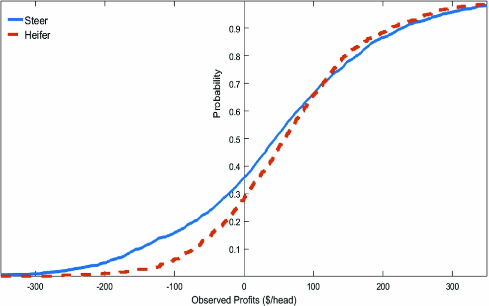
Figure 1. Empirical Distributions for the Observed Net Returns of Retaining Ownership of Steers and Heifers (excluding death loss)
5.2. Regression Results
All fixed and random effects in the regression model were significant in explaining net returns (P < 0.01) (Table 4). Higher average daily gain and lower feed-to-gain ratio increased net returns. This was expected given that previous research has also found that a lower feed-to-gain ratio and higher average daily gain (i.e., superior cattle performance) had a positive effect on retained ownership profitability (Jones et al., Reference Jones, Mintert, Langemeier, Schroeder and Albright1996; Lewis et al., Reference Lewis, Griffith, Boyer and Rhinehart2016; Mark, Schroeder, and Jones, Reference Mark, Schroeder and Jones2000; Schroeder et al., Reference Schroeder, Albright, Langemeier and Mintert1993). For a one-unit decrease in the feed-to-gain ratio, net returns to retained ownership increased by $55/head, and for a one-unit increase in average daily gain, retained ownership net returns increased $49/head. As expected, the number of individual health treatments received by the cattle was negatively associated with net returns. If an animal needed an additional health treatment, net returns decreased by $26/head. A higher dressing percentage also resulted in a higher net return, ceteris paribus. Previous research has also found that dressing percentage had a positive effect on retained ownership profitability (Lewis et al., Reference Lewis, Griffith, Boyer and Rhinehart2016; Mark, Schroeder, and Jones, Reference Mark, Schroeder and Jones2000; Schroeder et al., Reference Schroeder, Albright, Langemeier and Mintert1993).
Table 4. Parameter Estimates for Retained Ownership Net Returns ($/head) of Cattle Originating from Tennessee and Shipped to Iowa Feedlot

Notes: n = 2,953. Dependent variable is retained ownership net returns ($/head). Asterisk denotes significance at the 1% level. The restricted log-likelihood is −16,903.60. Likelihood-ratio tests supported the inclusion of the three random effects in the model.
A $1 increase in the corn price caused retained ownership net returns to decrease by $61/head. On average, returns to retaining ownership of heifers were $74/head greater than returns to retaining ownership of steers, which could be partially attributed to total feedlot costs being higher for steers than heifers (Table 2). Furthermore, previous research has also found that although steers have been shown to have higher average daily gain and lower feed conversion rates than heifers, they have also been shown to have higher death loss and veterinary costs than heifers (Belasco, Ghosh, and Goodwin, Reference Belasco, Ghosh and Goodwin2009). Days on feed had a positive effect on profits. This may be explained by more days on feed causing the animal to receive a higher quality grade, generating more revenue through a higher price received. Additionally, Lewis et al. (Reference Lewis, Griffith, Boyer and Rhinehart2016) found that days on feed was positively associated with profits when corn prices were low and was negatively associated with profits when corn prices were high. Placement weight positively affected retained ownership profits by $26/head for an additional 100 pounds at placement. This is consistent with recent trends in the cattle market that indicate cattle are being placed at heavier weights (USDA, Economics, Statistics and Market Information System, 2017). Lewis et al. (Reference Lewis, Griffith, Boyer and Rhinehart2016) also found retained ownership to be more profitable than selling calves as the placement weight of the animal increases.
Previous research by Mark, Schroeder, and Jones (Reference Mark, Schroeder and Jones2000), regarding steers in a Kansas feedlot from 1980 through 1997, indicated that steers placed on feed in late spring to early summer were generally more profitable than steers placed on feed in late winter and early spring. This research found that cattle placed on feed in summer were least profitable, whereas cattle placed on feed in winter were the most profitable (Table 4). For example, net returns were $131/head more for cattle placed in the winter compared with the spring.
5.3. Simulation Analysis Results
The unconditional observed net returns by placement season and the predicted net returns by placement season conditioned on the random effects in equation (3) appear in Table 5. The predicted net returns are a linear combination of the parameter estimates from equation (3) and the 2,953 cattle observations. Winter was the most profitable placement month for retained ownership, and summer was the least profitable placement season for retained ownership by examination of both the observed and predicted net returns. The unconditional observed distributions of net returns appear in the top panel of Figure 2, and the conditional distributions of net returns by placement season appear in the bottom panel of Figure 2. The differences between the observed and predicted net returns may be attributed to the fact that the predicted net returns are conditioned on the random effects of year, feedlot, and producer.
Table 5. Summary Statistics for Observed and Predicted Net Returns ($/head) of Cattle Placed on Feed in Different Seasons

a CV is the coefficient of variation (standard deviation/mean).
b L05 represents the 5th percentile.
c U95 represents the 95th percentile.
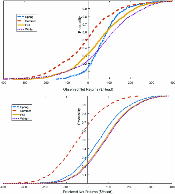
Figure 2. Cumulative Distributions for the Observed and Predicted Net Returns of Cattle Placed in Different Seasons
Under scenario 1 (the baseline scenario), retaining ownership of cattle in the winter was the most profitable with an average return of $86.62/head, and retained ownership in the summer was the least profitable with an average loss of $44.39/head (Table 6). The stochastic dominance analysis indicated that winter dominated all other placement seasons in the first degree, with the highest mean net return and the greatest probability of retained ownership being profitable (99.46%) followed by fall ($81.67/head, 99.22%) and spring ($56.04/head, 94.67%) (Figure 3). All placement season net return distributions were significantly different according to the K-S test (P < 0.01).
Table 6. Summary Statistics for Simulated Net Returns ($/head) of Cattle Placed in different Seasons under Four Scenarios

a CV is the coefficient of variation (standard deviation/mean).
b L05 represents the 5th percentile.
c U95 represents the 95th percentile.
d Scenario 1: simulated net returns ($/head) when all independent variables are at the mean.
e Scenario 2: simulated net returns ($/head) when corn price is at the 75th percentile, ceteris paribus.
f Scenario 3: simulated net returns ($/head) when average daily gain (ADG) and dressing percentage are at the 75th percentile, and number of health treatment and feed-to-gain ratio are at the 25th percentile, ceteris paribus.
g Scenario 4: scenarios 2 and 3 combined.
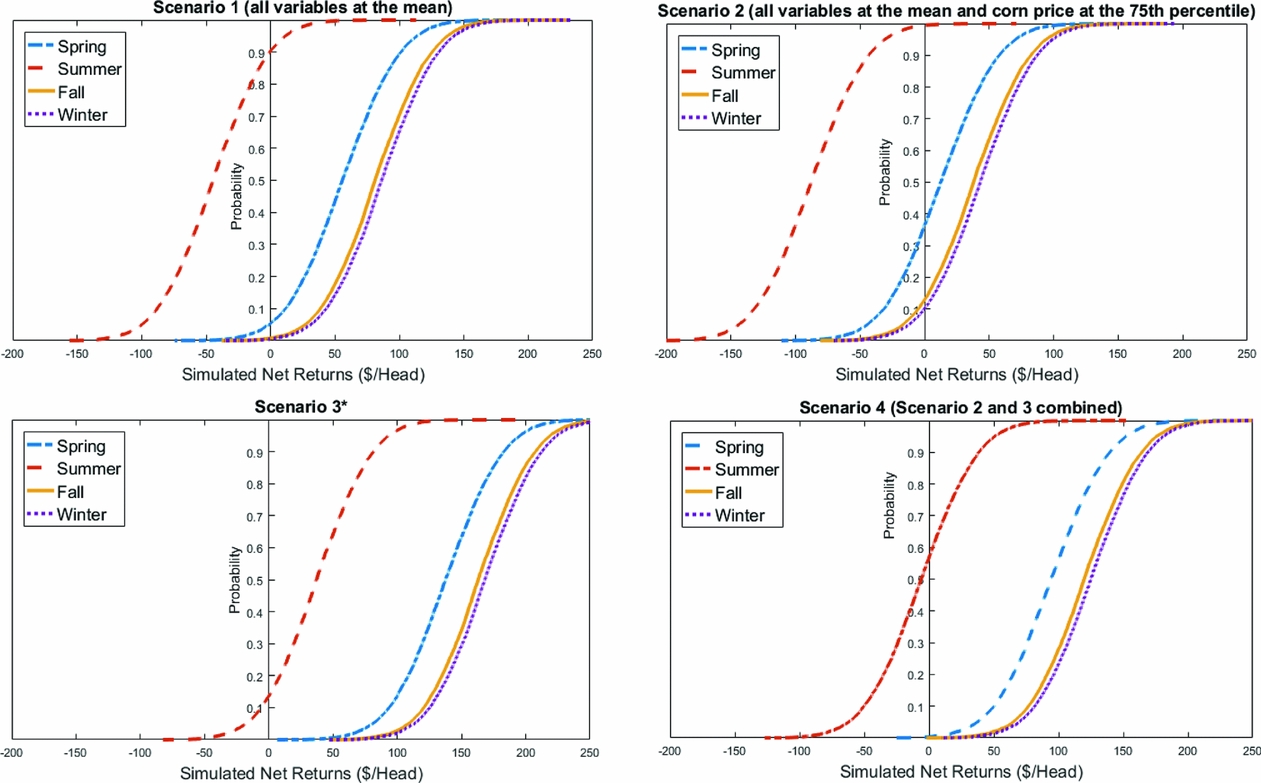
Figure 3. Cumulative Distributions for the Simulated Net Returns of Cattle Placed in Four Seasons under Four Scenarios (note: asterisk indicates that under scenario 3, dressing percentage and average daily gain were at the 75th percentile, and health treatments and feed-to-gain ratio were at the 25th percentile; all other variables were evaluated at their means)
When corn prices were increased from their mean ($4.52/bu.) to the 75th percentile ($5.22/bu.) in scenario 2, net returns and the probability of retained ownership being profitable decreased (Table 6, Figure 3). Stochastic dominance results indicated that winter remained first-degree dominant, with the highest net returns ($43.28/head) and the greatest likelihood of retained ownership being profitable (89.82%), followed by fall ($38.33/head, 87.09%), and spring ($12.70/head, 63.50%). The placement season net returns distributions were significantly different according to the K-S test (P < 0.01).
For scenario 3, net returns were simulated when the number of health treatments and feed-to-gain ratio were held at the 25th percentile, while average daily gain and dressing percentage were simulated at the 75th percentiles (i.e., superior cattle performance scenario). Retained ownership of cattle placed in the spring, fall, and winter were always profitable (Figure 3). Mean net returns of cattle placed in the winter were the highest ($168.47/head), followed by the fall ($163.52/head) and spring ($137.89/head) (Table 6). Retained ownership was profitable 86.38% of the time for cattle placed in the summer with a mean net return of $37.47/head. Similar to the other scenarios, winter dominated the other placement seasons by the first degree. The placement season net return distributions were significantly different according to the K-S test (P < 0.01).
In scenario 4 (combination of scenarios 2 and 3), the winter placement decision dominated the other seasons by the first-degree dominance criteria, with an average net return of $125.13/head (Table 6). Retained ownership was profitable 100% of the time for cattle placed in the winter (Figure 3). Fall was the second most profitable season for retained ownership with an average net return of $120.18/head and was profitable 99.99% of the time. Spring was the third most profitable season for retained ownership with an average net return of $94.55/head and was profitable 99.70% of the time. Retained ownership in the summer resulted in an average net loss of $5.87/head and was profitable only 43.17% of the time. The placement season distributions were all significantly different from each other according to the K-S test (P < 0.01).
Overall, a comparison of the scenarios exhibited how feed costs, cattle characteristics, and feedlot performance played a role in affecting retained ownership net returns. Winter was the dominant placement season with the highest profitable percentage throughout the four scenarios followed by fall and spring. Summer was the least preferred placement season with the lowest probability of cattle being profitable. The ranking list of placement season alternative by simulation was consistent with the mixed model results.
6. Summary and Conclusions
Profits in the cattle industry have been highly volatile in recent years (Betchel, Reference Betchel2016) making it critical for cattle producers to understand which marketing strategies are the most profitable. Research prior to 2000 indicated that retained ownership could be a profitable marketing strategy for cow-calf producers in most years (Fausti et al., Reference Fausti, Johnson, Epperson and Grathwohl2003; Lawrence, Reference Lawrence2005; Randall and Watt, Reference Randall and Watt1986; Wagner and Feuz, Reference Wagner and Feuz1991; Watt, Little, and Petry, Reference Watt, Little and Petry1987), but little research has been carried out on this question since the turn of this century. Accordingly, the research reported here investigated whether retained ownership is a profitable marketing alternative for cow-calf producers and found that producers could capture profits. From 2005 through 2015, net returns to retained ownership including death loss were positive in 8 of the 11 years, with an average return of $35/head. Furthermore, when excluding death loss, 72% of the heifers retained were profitable and 64% of the steers retained were profitable.
A mixed model was used to determine how cattle performance and producer choice variables affect retained ownership profitability. Improved animal characteristics (lower feed-to-gain ratio, increased average daily gain, increased dressing percentage, and reduced number of health treatments) led to increased retained ownership net returns. This result was confirmed using simulation analysis. For example, almost all animals retained were profitable under scenario 3 (superior animal characteristics). Therefore, cow-calf producers interested in retained ownership would benefit the most by retaining ownership of the animals with the best characteristics.
Increased placement weight, increased days on feed, and decreased corn prices increased retained ownership net returns. Therefore, producers would benefit the most by retaining ownership of cattle when corn prices are low. As cattle were heavier, they were more profitable to retain through the feedlot than to sell as feeder cattle as evidenced by an increased placement weight being associated with higher net returns to retained ownership. This finding may be explained by the opportunity cost calculation. Opportunity cost was calculated using USDA-AMS weekly auction data from Tennessee. Heavy feeder cattle (i.e., greater than 800 pounds) are often discounted in Tennessee because there are very few heavy animals going through the marketplace, which makes it difficult to piece together a truckload lot (48,000 to 50,000 pounds) of similar animals. Producers would also benefit by keeping their cattle on grain longer if they retain ownership of them.
Heifers were more profitable to retain ownership of than steers. Though heifers were more profitable than steers, one shortcoming of this research was the small sample size of heifers relative to steers. Of the heifers that entered into the feedlot from 2005 through 2015, nearly 81% of them were retained from 2007 through 2010, whereas only 58% of steers were marketed to the feedlot in those same years. Winter, fall, and spring were more profitable placement seasons than summer. This finding is potentially a result of feeder cattle prices in the summer being higher than the other three placement seasons, which increased the opportunity cost calculation. Similar to the heifer result, this could partially be driven by the specific sample size of the particular placement seasons. Simulation analysis examined retained ownership profitability by placement season under different feed and animal characteristic scenarios. Regardless of scenario, winter was the most profitable placement season to retain ownership followed by fall and spring.
This research contributes to the literature by examining retained ownership profitability from 2005 through 2015. Given retained ownership was a profitable marketing strategy over this time, and during years prior to 2000, it is likely that retained ownership will remain a profitable marketing opportunity for cow-calf producers in the future. However, a limitation of this research is that cattle prices were primarily increasing in the years examined, which would lead to retained ownership being a profitable marketing strategy simply because of capturing additional profits added by price increases. Therefore, future research could use cattle future contract prices to control for movement in cattle prices to determine the profitability of retained ownership holding cattle prices constant. Future research could also examine how the relationship between feeder and fed prices affects retained ownership profitability, and it could assess retained ownership profitability in different regions of the country. Finally, this research provides useful information that can be used by extension personnel and cattle producers interested in the profitability of retained ownership as a marketing strategy.


 Open access