


1. INTRODUCTION
The Greenland ice sheet (GrIS) is sensitive to a warming climate, as surface melting is a major element of its mass budget (Rignot and others, Reference Rignot2011). Ice volume reconstructions reveal that past climate changes affected the GrIS massively: Greenland's ice volume experienced changes of ~5–9 m sea-level equivalent (SLE) since the last interglacial's peak sea level (Vasskog and others, Reference Vasskog2015). The total present-day volume of the GrIS, in comparison, is of the same order of magnitude (~7.4 m SLE).
To interpret historic and recent mass changes of the GrIS, it is necessary to quantify the components of the surface mass balance (SMB), which primarily are surface melt, accumulation and refreezing. Direct measurements of surface melt rates are only available at isolated locations and until recently were not designed to cover more than a few years. Over the last decade, however, a network of automatic mass-balance stations has been established to monitor the annual mass loss of the GrIS (Ahlstrom and others, Reference Ahlstrom2008). Since 2002, the Gravity Recovery and Climate Experiment (GRACE) (Tapley and others, Reference Tapley2004) satellite mission allows to detect integral mass changes of the GrIS (Wouters and others, Reference Wouters2014), but additional data are necessary to separate and quantify the individual SMB components such as surface melt (Sasgen and others, Reference Sasgen2012; Tedesco and Fettweis, Reference Tedesco and Fettweis2012). In particular, high-resolution regional climate models such as the Regional Atmospheric Climate Model (RACMO) (Noel and others, Reference Noel2015) or the Modèle Atmosphérique Régional (MAR) (Fettweis and others, Reference Fettweis2017) allow for a separation of the SMB.
Where high-resolution modelling is not feasible, a common approach is to estimate surface melt rates, M with realizations of the positive degree-day (PDD) model formulated for example in Reeh (Reference Reeh1989). The term PDD refers to the temporal integral of near surface temperatures T exceeding the melting point, sampled at daily or higher frequency. The PDD scheme linearly relates PDDs to snow and ice melt through respective empiric degree-day factors (DDF) in the form M = DDF × PDD. Following Braithwaite (Reference Braithwaite1985), PDD values are commonly approximated from monthly mean temperatures (or, from annual mean and mean July temperatures based on a sinusoidal seasonal cycle, Reeh (Reference Reeh1989)), assuming that on sub-monthly timescales temperatures are normally distributed around the monthly mean temperatures with a standard deviation, σ. One benefit of this approach is its simplicity, as it only requires information about near surface air temperature. Even spatially incomprehensive or coarse resolution temperature data still permit some rough estimate of the surface melt rates, as temperatures can be downscaled via lapse rate corrections. The PDD model has been thus applied to estimate surface melt rates from coarse resolution climate simulations (e.g. Charbit and others, Reference Charbit2013; Heinemann and others, Reference Heinemann2014; Roche and others, Reference Roche2014; Ziemen and others, Reference Ziemen, Rodehacke and Mikolajewicz2014; Gierz and others, Reference Gierz, Lohmann and Wei2015) or, extending the instrumental record into the past, from temperature reconstructions deduced from ice cores (e.g. Box, Reference Box2013; Wilton and others, Reference Wilton2017). In many such applications σ is assumed to be constant in time and space and then σ commonly is chosen in the range 4.5–5.2°C. Fausto and others (Reference Fausto2009) pointed out that the ablation zone of the GrIS exhibits a considerably smaller variability during the melting season with σ T ranging between 1.7 and 2.9°C. Consequently, a growing number of studies approximate PDDs using spatially or temporally variable σ (e.g. Roche and others, Reference Roche2014; Ziemen and others, Reference Ziemen, Rodehacke and Mikolajewicz2014; Contoux and others, Reference Contoux2015; Wilton and others, Reference Wilton2017).
In modelling studies, the DDFs of snow and ice can be treated as convenient tuning parameters, which can be constrained by observed mass changes from satellite data. Also, many applications of the PDD model in Earth system modelling adopt DDFs of 3 and 8 mm °C−1 d−1 for snow and ice, respectively, following an approach, which was applied in a simulation of the GrIS dynamics by Huybrechts and others (Reference Huybrechts, Letreguilly and Reeh1991). Direct calibrations of DDFs, however, rely on the few available measurements of melt rates which often differ in sampling frequency and period. In a global compilation, Hock (Reference Hock2003) reviews DDF calibrations from ice sheets and glaciers, which exhibits a wide range of values for different locations indicating that DDFs strongly depend on parameters such as altitude, latitude or local conditions (e.g. debris cover, liquid water content, shading). For Greenland DDF estimates for ice range from 5.8 to 12 mm °C−1 d−1 for stations at altitudes lower than 1000 m a.s.l., while measurements at higher elevations yield values of up to 20 mm °C−1 d−1. According to a calibration to long-term measurements and energy-balance modelling from southern Greenland (Johannesson and others, Reference Johannesson, Sigurdsson, Laumann and Kennett1995) most applications employ for snow DDF ~3 mm °C−1 d−1 for Northern Hemispheric ice sheets. However, a calibration using data from two stations at 1020 m and 1520 m a.s.l. in Southwest Greenland suggests DDF of snow well above 20 mm °C−1 d−1 (van den Broeke and others, Reference van den Broeke, Bus, Ettema and Smeets2010). In consequence, recent studies have proposed modifications of the PDD method, which make use of temperature-dependent DDFs (Tarasov and Peltier, Reference Tarasov and Peltier2002; Greve, Reference Greve2005; Fausto and others, Reference Fausto2009).
Charbit and others (Reference Charbit2013) find that ice sheet simulations of the last glacial period exhibit a strong sensitivity to the realization of the PDD model. Specifically Charbit and others (Reference Charbit2013) compare schemes with constant (Reeh, Reference Reeh1989) or temperature dependant DDFs (Tarasov and Peltier, Reference Tarasov and Peltier2002; Fausto and others, Reference Fausto2009), using either PDD approximations based upon spatially variable (Fausto and others, Reference Fausto2009) or constant standard deviation (Reeh, Reference Reeh1989; Tarasov and Peltier, Reference Tarasov and Peltier2002). Rogozhina and Rau (Reference Rogozhina and Rau2014) evaluate a similar selection of PDD model realizations with respect to their ability to reproduce Greenland's surface melt rates of the years 1958–2001 as simulated from the regional climate – snow pack model RACMO in combination with GRACE ice mass measurements. Rogozhina and Rau (Reference Rogozhina and Rau2014) find a good agreement with the surface melt rates of the regional model if spatially variable standard deviations are combined with the parameterization of Fausto and others (Reference Fausto2009). The other combinations exhibit a strong, but mostly temporally constant bias.
In this study, we aim to fathom principles behind heterogenous DDF calibrations. Direct observations are still spatially sparse, rarely cover more than a decade and may be influenced by local conditions which are not representative on a larger scale. For a comprehensive analysis we thus use a simulation of Greenlands climate of the years 1948–2016 with the state-of-the-art regional climate and snow pack model MAR (Fettweis and others, Reference Fettweis2017) as a reference. We consider and evaluate three PDD model realizations, which differ in the way that temperature variability is represented, and calibrate these individually. We optimize the calibration on the basis of the first 25 years of the reference simulation. We first investigate the spatial properties of DDFs if locally calibrated. We then determine ideal Greenland-wide parameterization for each formulation and test their skill to reproduce MAR surface melt rates in their spatial characteristics and evolution, using the MAR temperatures as input.
2. METHODS
2.1. The modèle atmosphérique régional
We use outputs from version 3.5 of the MAR regional climate model applied over the GrIS for calibration and evaluation of different PDD-model realizations. The MAR, is a coupled land-atmosphere regional climate model featuring an atmospheric model (Fettweis, Reference Fettweis2007; Reijmer and others, Reference Reijmer2012) and including a snow pack component. The simulation considered here is analyzed in detail in Fettweis and others (Reference Fettweis2017). The simulation covers Greenland and surrounding areas at a 20 km spatial resolution, forced at the lateral boundaries and ocean surface with reanalysis data from the National Centers for Environmental Prediction-National Center for Atmospheric Research (NCEP) for the years 1948–2016 (Kalnay and others, Reference Kalnay1996). MAR has been validated against satellite and in situ data (e.g. Lefebre and others, Reference Lefebre2005; Fettweis and others, Reference Fettweis2011) and has been used in multiple studies to simulate ice sheet and atmospheric parameters, such as SMB, surface melt and atmospheric circulation near Greenland (e.g. Fettweis and others, Reference Fettweis2011; Franco and others, Reference Franco, Fettweis and Erpicum2013; Tedesco and others, Reference Tedesco2013).
2.2. The PDD-model
A PDD model (Braithwaite, Reference Braithwaite1985; Reeh, Reference Reeh1989) allows estimating the monthly surface melt rates from temperatures T sampled at daily or higher frequency. The PDD is here defined to be the cumulative temperature exceeding melting point T + (with T + = max(T, T 0), T 0 = 0°C) throughout a time interval [t 0, t 1]
 $$ PDD = \int_{t0}^{t1} {T^ +} (t) dt. $$
In practice, temperatures will be sampled or simulated with discrete time steps Δt and are often only available on monthly or longer timescales. Therefore, we focus on realizations of the PDD model that approximate PDD based on monthly statistics following an approach from Braithwaite (Reference Braithwaite1985): assuming that temperatures are normally distributed around monthly or climatologic mean temperatures T̄, the PDD of a given month can be approximated as
 $$ {PDD}\left({\bar T},\sigma\right) = {\displaystyle{\Delta t} \over {\sigma\sqrt{2\pi}}} \int_0^\infty {Texp\left(-{\displaystyle{(T - {\bar T})^{2}} \over {2\sigma^{2}}}\right) dT}, $$
with Δt = 1 month.
Here, we consider surface melt estimates of the form
 $$ M = {\rm DDF} \times {PDD}({\bar T}, \sigma), $$
and distinguish between snow and ice melt by applying distinct constant DDF for snow and ice, respectively. The surface melt of a given month is considered in two phases: any surface layer of snow must be melted, before the subjacent ice is melted with the remaining PDD that is not used up by snow melt.
We consider different options to represent unresolved temperature variability by σ. We focus on the slush zone below the runoff line, which is here defined to be the region where mean surface melt rates M exceed refreezing rates. In Greenland the runoff line is usually positioned above the equilibrium line where ablation and accumulation balance.
In the first instance, we consider two approximations, PDDVAR = PDD(T̄, σVAR(x, t)) and PDDCONST = PDD(T̄, σCONST = 5°C) and compare these with PDD6h, which is directly calculated from 6-hourly temperatures according to (1). Here, T̄ are monthly mean temperatures from the MAR simulation and σ VAR represents its monthly temperature variability calculated at each grid point by combining the monthly mean of the daily temperature amplitude dT day = 0.5 (T̄ max − T̄ min) and the standard deviation of the daily mean temperatures throughout a month, σmonth, according to:
 $$ \sigma_{\rm VAR} = \sqrt{(\sigma_{\rm month}^2 + (0.564 \; dT_{\rm day})^2)}. $$
The factor 0.564 in this equation is somewhat smaller than what would be assumed for a sinusoidal daily cycle and was determined from the MAR calibration period by optimizing the regression between PDDVAR = PDD(T̄, σVAR) and the PDD6h from 6-hourly temperature data. Additionally, we consider PDDEFF = PDD(T̄, σEFF) with
 $$ \sigma_{\rm EFF} = \sqrt{(\sigma_{{\rm month}}^2 + (0.564 \; {\max}[dT_{\rm day},{5}^{\circ} {\rm C}])^{2})} $$
assuming that daily temperature amplitude never falls below 5°C. This approximation aims to eliminate a negative feedback that may influence the temperature–melt relation if mean temperatures approach melting point: in this case, not only do temperature variations induce surface melt, but, on the other hand, surface melt (or refreezing) dampens temperature variations. This feedback is particularly prominent in the diurnal variability. If surface melt occurs, the maximum (daytime) temperature will be lowered due to latent heat flux and likewise minimum (nighttime) temperatures will be increased due to refreezing meltwater. In the MAR simulation we find, that above melting surfaces daily temperature amplitude declines from ~5°C–1.5°C when monthly mean temperatures approach melting point from both directions (Fig. 1). σ EFF can be understood as a rough estimate of an ‘effective’ temperature variability, freed from the dampening effect of phase transitions on the daily temperature amplitude. Unlike parameterizations that aim to explicitly resolve the low variability in the ablation zone (Fausto and others, Reference Fausto, Ahlstrom, Van As and Steffen2011; Seguinot and Rogozhina, Reference Seguinot and Rogozhina2014; Wake and Marshall, Reference Wake and Marshall2015), this parameterization raises the low variability in the ablation zone to suppress the effect of negative feedbacks.

Fig. 1. Multiyear monthly mean daily temperature amplitude averaged over the first 25 years of the MAR simulation (calibration period) against respective multiyear monthly mean temperatures. The size of each point is scaled by the surface melt rate, colours reflect standard deviation of daily mean temperatures throughout July; grid points with melt rates M < 2 mm d−1 are not represented.
Parameterizing variability by =5°C, as applied in PDDCONST, strongly overestimate variability. In summer, σ VAR rather takes values ~2°C–3.5°C below the runoff line (Fig. 2, left). Applying a lower bound on daily temperature amplitudes (PDDEFF) essentially increases σ EFF by 1–1.6°Cd−1 below the runoff-line compared with σ VAR (Fig. 2, right). At high elevation or outside of the melt season σ EFF and σ VAR are almost identical .

Fig. 2. July σ VAR (left) and σ EFF (right) averaged over the first 25 years of the MAR simulation (calibration period). Black contour indicates the runoff line.
In consequence, PDDVAR agrees well with PDD6h, whereas PDDCONST reveals a strong bias relative to PDD6h which is particularly pronounced for small values and dominantly positive for PDD6h > 2°C d−1. The bias in PDDEFF is less pronounced but also in the main positive (Fig. 3).
Fig. 3. PDDVAR (a), PDDCONST (b) and PDDEFF (c) as functions of PDD6h. Identity is displayed as a grey line in all panels for comparison.
2.3. Calibration of the PDD model
In this study, we first calibrate DDFs for each grid point individually before a Greenland-wide calibration is considered in later sections. We calibrate DDFs for snow and ice and for each PDD approximation (DDFVAR, snow, DDFCONST, snow, DDFEFF, snow, DDFVAR, ice, DDFCONST, ice, DDFEFF, ice). For calibration, we use monthly means of the different approximations of PDD together with the local snow height (SNH), snow fall (SF) and melt rates, M MAR from the MAR simulation. We consider a 25-year calibration period a suitable choice. Relative to parameters obtained from a 69-year calibration period (i.e. the length of the simulation), errors of <10, 5, 3 and 2% are obtained for periods longer than 3, 6, 16 and 54 years (not shown). Thus, a 25-year period offers a reasonable accuracy, while the remaining 44 years allow to assess the temporal stability of the individual realizations. We determine snow melt M MAR, snow as
 $$ M_{\rm MAR, snow} = {\min} \left({\displaystyle{\rm SNH} \over {dt}} + {\rm SF},M_{\rm MAR}\right),\quad dt = 1 \, {\rm month} $$
and ice melt as
 $$ M_{\rm MAR, ice} = M_{\rm MAR} - M_{\rm MAR,\rm snow}. $$
To determine DDF of snow locally at a grid point i, we identify those months, ms, in which snow melt is predominant (M MAR, ice ≈ 0, PDD,snow ≈ PDD) and use these to obtain a local calibration,
 $$ {\rm DDF}_{,{\rm snow}}(i) = {\displaystyle{\sum \nolimits_{ms} M_{\rm MAR}(i,ms)} \over {\sum \nolimits_{ms} {\rm PDD}(i,ms)}}, $$
for all glaciated grid points i. As the calibration becomes inaccurate where substantial surface melting does not occur on a regular basis, we reject the local calibration as meaningless where PDDs accumulated over the 25-year period do not exceed 10°C d−1. For a Greenland-wide calibration we modify this method as
 $$ {\rm DDF}_{,{\rm snow}} = {\displaystyle{\sum \nolimits_{i,ms} M_{\rm MAR}(i,ms)} \over {\sum \nolimits_{i,ms} {\rm PDD}(i,ms)}}. $$
In a second step, we can consider all months m and all grid points i to calibrate DDF of ice. Where melt rates are large enough to remove the snow cover and melt subjacent ice, we determine the proportion of PDD, which is available for ice melt as
 $$ {\rm PDD}_{,{\rm ice}}(i,m) = {\rm PDD}(i,m)-{\rm PDD}_{,{\rm snow}} $$
with
 $$ {\rm PDD}_{,{\rm snow}}(i,m) = {\displaystyle{M_{\rm MAR, snow}}(i,m) \over {\rm DDF}_{,{\rm snow}}(i)}, $$
DDF of ice is then analogously to DDF,snow calibrated locally as
 $$ {\rm DDF}_{,{\rm ice}}(i) = {{\displaystyle{\sum \nolimits_{m} M_{\rm MAR, ice}}(i,m)} \over {\sum \nolimits_{m} {\rm PDD}_{,{\rm ice}}(i,m)}}, $$
for all grid points that meet the condition that PDD,ice integrated over the 25-year period exceeds 10°Cd−1. Analogously, for the Greenland-wide calibration this method is modified as in Eqn (9).
3. RESULTS
3.1. Influence of temperature variability on locally-calibrated parameters
As outlined above, we locally calibrate DDFs for snow and ice based on PDDCONST, PDDVAR and PDDEFF. We find a strong sensitivity of DDFs on the individual PDD approximation (Fig. 4).

Fig. 4. Spatial distribution of DDF,snow (upper panels) and DDF,ice (lower panels) as calibrated locally based on PDDVAR (left panels), PDDCONST (center panels) and PDDEFF (right panels). The black contour line indicates the runoff line which limits the slush zone as defined in the text.
Using PDDVAR for calibrations yields the strongest spatial heterogeneity with DDFVAR, snow and DDFice mostly ranging from 3 to 40 mm °C−1 d−1 in the slush zone. In contrast, the calibration based on PDDEFF and PDDCONST yields more homogenous distribution in the slush zone. DDFEFF, snow and DDFEFF, ice mostly remain in the range between 2.5–15 mm °C−1 d−1 and DDFCONST, snow and DDFCONST, ice in the range from 2 to 10 mm °C−1 d−1.
DDFs calibrated for the realization with constant standard deviation (DDFCONST) exhibit primarily a latitudinal dependence (Figs 4, 5). If the realization incorporates the local standard deviations (DDFVAR), calibrations primarily appear to be strongly temperature-dependent with higher DDFs at lower temperatures, while some latitudinal dependence persists. Parameters in the realization with lower bounded daily temperature variability (DDFEFF) also exhibit a combination of temperature dependence, which is not as pronounced as in the DDFVAR, and latitudinal dependence.

Fig. 5. DDF,snow (upper panels) and DDF,ice (lower panels) as calibrated locally based on PDDVAR (left panels), PDDCONST (center panels) and PDDEFF (right panels) as functions of the local climatologic July temperature, T July, of the calibration period. Each scatter point represents one grid point in the slush zone, colors reflect latitude.
3.2. Optimal parameters for Greenland-wide applications
To address the skill of different realizations of the PDD model we conduct a Greenland-wide calibration using all grid points that are within the domain of GrIS. Assuming a constant standard deviation we obtain DDFCONST, snow = 5.1 mm °C−1 d−1 and DDFCONST, ice = 5.4 mm °C−1 d−1 which is in the range of observation-based calibrations of high latitude ice sheets and glaciers. DDFEFF and DDFVAR are calibrated to 6.4 mm °C−1 d−1 and 10.8 mm °C−1 d−1 for snow and to 6.1 mm °C−1 d−1 and 8.1 mm °C−1 d−1 for ice, respectively. DDFsnow is not substantially smaller than DDFice, as it is in the local calibrations, because ice melt occurs largely at low elevations with relatively warm summer temperatures, while snow melt happens to largest parts under colder temperatures as in spring or higher elevations. The Greenland-wide calibration even results in DDF,snow ≥ DDF,ice for formulation VAR and EFF. An overview of the Greenland-wide DDFs is presented in Table 1.
Table 1. Overview of PDD model realizations. The evaluated realizations are based on approximations of PDD which differ in the representation of sub-monthly variability σ and in greenland-wide calibrated degree-day factors DDF,snow and DDF,ice. RMSEtime is the root mean square error of the 1948–2016 total Greenland surface melt predictions (Fig. 7) relative to the MAR simulation. RMSEspace is the root mean square error of predicted mean surface melt rates in the slush zone during the calibration period (Fig. 9) relative to the MAR simulation
Additional to the three optimally calibrated realization we define the fourth realization which is also based on PDDVAR but which include temperature-dependent instead of constant Greenland-wide parameters to better match the local calibrations (Fig. 6). Using an analogue approach to the parameterization proposed by Fausto (Reference Fausto2009) we find a good fit of the locally calibrated DDF,snow with
 $$\eqalign{& {\rm DD}{\rm F}_{{\rm VARF},{\rm snow}} = \cr & \left\{ {\matrix{ {\beta _{{\rm snow}}^w } \hfill & {T_{{\rm July}} \ge T_w} \cr {\beta _{{\rm snow}}^w + \displaystyle{{\beta _{{\rm snow}}^c - \beta _{{\rm snow}}^w } \over {(T_w - T_c)}}(T_{{\rm July}} - T_c)} & {T_c \le T_{{\rm July}}{\rm < }T_w} \cr {\beta _{{\rm snow}}^c } \hfill & {T_{{\rm July}}{\rm < }T_c{\rm }} \cr } } \right.} $$
and DDF,ice with the third-order polynomial:
 $$\eqalign{& {\rm DD}{\rm F}_{{\rm VARF},{\rm ice}} = \cr & \left\{ {\matrix{ {\beta _{{\rm ice}}^w ,} \hfill & {T_{{\rm July}} \ge T_w} \cr {\beta _{{\rm ice}}^w + \displaystyle{{\beta _{{\rm ice}}^c - \beta _{{\rm snow}}^w } \over {{(T_w - T_{{\rm July}})}^3}} * ({(T_w - T_{{\rm July}})}^3),} & {T_c \le T_{{\rm July}}{\rm < }T_w} \cr {\beta _{{\rm ice}}^c ,} \hfill & {T_{{\rm July}}{\rm < }T_c} \cr } } \right.} $$
with T July being the mean July temperature and  $\beta ^{w}_{\rm snow} = 5\,{\rm mm}\,^{\circ}{\rm C}^{-1}\,{\rm d}^{-1}$, $\beta ^{c}_{\rm snow} = 14\,{\rm mm}\,^{\circ}{\rm C}^{-1}\,{\rm d}^{-1}$, $\beta ^{w}_{{\rm ice}} =6\,{\rm mm}\,^{\circ}{\rm C}^{-1}\,{\rm d}^{-1},\, \beta ^{c}_{{\rm ice}} = 20\,{\rm mm}\,^\circ {\rm C}^{-1}\,{\rm d}^{-1}$, T w = 6°C and T c = −1°C (Fig. 6) compared with the parameters $\beta ^{w}_{\rm snow} = \beta ^{w}_{\rm snow} = 3\,{\rm mm}\,^\circ {\rm C}^{-1}\,{\rm d}^{-1}$ and $\beta ^{w}_{{\rm ice}} = 7\,{\rm mm}\,^\circ {\rm C}^{-1}\,{\rm d}^{-1},\, \beta ^{c}_{{\rm ice}} = 15\,{\rm mm}\,^\circ {\rm C}^{-1}\,{\rm d}^{-1}$, T w = 10°C and T c = −1°C in Fausto (Reference Fausto2009).
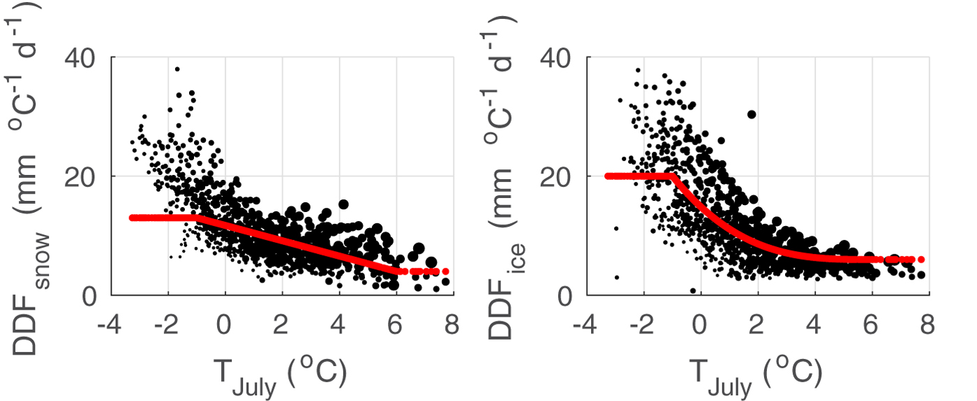
Fig. 6. Temperature dependency of DDFVARF, snow (left, red) and DDFVARF, ice (right, red) in comparison with the respective local calibration DDFVAR(i) (black) for all grid points i in the slush zone (Fig. 5, left panels). The size of scatter points reflects annual mean surface melt.
We thus consider four realizations of the PDD model,
 $$\eqalign{& M_{\rm VAR} = {\rm DD}{\rm F}_{\rm VAR} \times {\rm PD}{\rm D}_{\rm VAR}, \cr & M_{\rm CONST} = {\rm DD}{\rm F}_{\rm CONST} \times {\rm PD}{\rm D}_{\rm CONST}, \cr & M_{\rm EFF} = {\rm DD}{\rm F}_{\rm EFF} \times {\rm PD}{\rm D}_{\rm EFF}, \cr & M_{\rm VARF} = {\rm DD}{\rm F}_{\rm VARF} \times {\rm PD}{\rm D}_{\rm VAR},} $$
which allow to estimate monthly surface melt rates from monthly climate variables of the MAR simulation, i.e. from monthly mean temperatures T̄, monthly standard deviation of daily mean temperatures σ month, monthly mean daily temperature amplitude, dT, snow height, SNH and snow fall, SF.
3.3. Evaluation of Greenland-wide applications
The MAR simulation covers the years 1948–2016 and, averaged over this 69-year period, hindcasts a total annual Greenland surface melt of 489 Gt. In the first 50 years of the simulation, the total surface melt never exceeds 600 Gt (Fig. 7a). Towards the end of the simulation, surface melt intensifies and exceeds 600 Gt in 7 out of the last 19 years. As this intensification is not covered by the calibration period, total annual Greenland surface melt during the first 25 years amounts to 467 Gt on average (Fig. 8). The year 2012 of the simulation exhibits an exceptional melt of 987 Gt and exceeds all other years of the simulation by more than 200 Gt. Together with snow fall and refreezing this corresponds to a net surface mass loss of 427 Gt over the summer months. By comparison, the GRACE measurements indicate a total summer mass loss (including marine discharge) of 628 ± 96 Gt (Tedesco and others, Reference Tedesco2013). In observations, the 12 of July 2012 stands out due to an extreme melt event which affected almost the entire surface of the GrIS (Nghiem and others, Reference Nghiem2012).

Fig. 7. (a) Total Greenland surface melt from 1948 to 2016 as simulated by MAR (M MAR, black) and predicted from M VAR (green), M CONST (red), M EFF (blue) and M VARF (cyan). (b) relative yearly bias of M VAR (green), M CONST (red), M EFF (blue) and M VARF (cyan) 1948–2016 relative to M MAR .
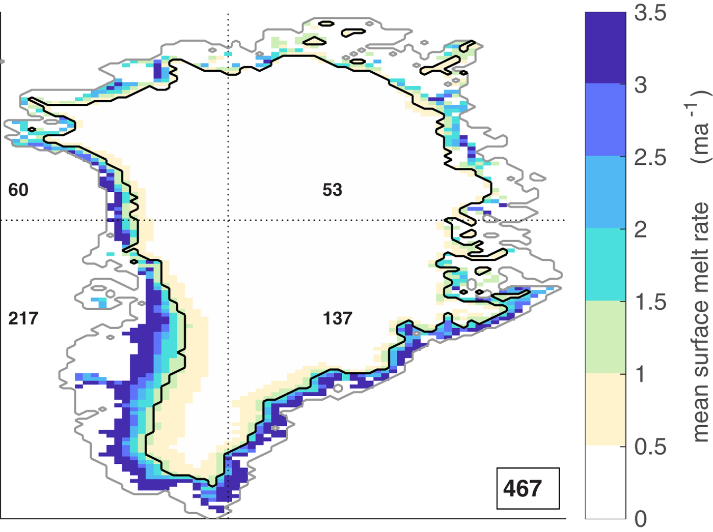
Fig. 8. Mean yearly Greenland surface melt of the calibration period (years 1948–1972), as simulated by MAR. The black contour indicates the upper boundary of the slush zone. Numbers refer to the respective spatially-integrated yearly mean surface melt in the four sectors which are separated by the dotted lines and the mean total surface melt (lower right corner) in Gt.
We find that all four realizations generally capture the yearly evolution of the total yearly Greenland surface melt. Within the 69 years of the simulation the relative bias exceeds ± 10% in 5, 6 and 4 years for M VAR, M CONST, M EFF, respectively, but in 20 years for M VARF (Fig. 7b). M CONST particularly fails to reproduce the extreme melt in year 2012 with a bias of 180 Gt. There is no indication, however, that M CONST becomes increasingly unreliable with the intensifying surface melt towards the end of the simulation. The root mean square error, RMSEtime of the surface melt hindcast is smallest for M EFF and largest for M VARF (Table 1). In general, all four realizations reproduce the melt evolution relatively well. We want to stress, however, that surface melt estimates will be heavily offset if the calibration is not adapted to the PDD formulation: DDFVAR × PDDCONST or DDFCONST × PDDVAR produce a relative bias of ≈ 100% and −50 %, respectively throughout the simulation (not shown).
Throughout the calibration period of the MAR simulation, surface melt M MAR is characterized by a narrow slush zone at the lower part of the GrIS with melt rates exceeding 3 m a–1 near the western and south-eastern coast (Fig. 8). The spatial distribution of surface melt is reasonably well represented in all four realizations. Figure 9 shows the respective mean local bias of surface melt rates with respect to surface melt rate from the MAR simulation (Fig. 8) averaged over the calibration period. Inherent to their design, the bias in total Greenland-wide surface melt hindcast vanishes for M VAR, M EFF and M CONST over the calibration period (Fig. 9); for M VARF the total bias does not vanish but is small (≈1 Gt). Outside of the calibration period the spatial pattern remains generally the same while the total bias depends on the selected evaluation period (not shown). All surface melt estimates, especially M CONST, tend to overestimate surface melt in northern Greenland and underestimate surface melt in southern Greenland, which is in line with the latitude-dependence found in the locally-calibrated DDFs (Fig. 5). A negative bias is particularly prominent in the ablation zone of south-western Greenland. In agreement with the temperature dependence found for the locally-calibrated DDFVARs (Fig. 5), M VAR tends to overestimate surface melt at low elevations and underestimate at high elevations. This is also reflected in a relatively large spatial root mean square of the surface melt distribuion in the slush zone averaged during the calibration period, RMSEspace (Table 1). The MAR simulation exhibits some residual surface melt rates in the interior of southern Greenland which usually do not exceed the refreezing rates and are thus negligible for the SMB (Fig. 8). It should be yet noted that only the realization incorporating local variability and temperature-dependent parameters (M VARF) is able to reproduce this melt at high altitudes due to its temperature-dependent parameterization. The extreme melt of the year 2012, which is characterized by intensified surface melt at high altitudes is thus better captured in M VARF than in the other realizations. Overall M VARF provides the best representation of local melt rates which is also reflected in the smallest RMSEspace as presented in Table 1.

Fig. 9. (a) Bias of M VAR prediction of Greenland surface melt to MAR simulation during the calibration period. (b) Same as (a) but for M CONST. (c) Same as (a) but for M EFF. (d) Same as (a) but for M VARF. The grey contour indicates the upper boundary of he slush zone. Numbers refer to the bias in the four sectors which are seperated by the dotted lines and the mean total surface melt (lower right corner) in Gt.
4. DISCUSSION AND CONCLUSION
The PDD model is used to estimate the surface melt of ice sheets by assuming that the relation between PDD and surface melt is linear. On a continental scale, however, this assumption appears not to be justified as model parameters were found to be spatially incoherent (Hock, Reference Hock2003) and in particular temperature-dependent (Tarasov and Peltier, Reference Tarasov and Peltier2002). Furthermore, previous studies have demonstrated that surface melt estimates derived from the PDD model are highly sensitive to the representation of sub-monthly temperature variability, for a given parameterization (Charbit and others, Reference Charbit2013; Seguinot, Reference Seguinot2013; Rogozhina and Rau, Reference Rogozhina and Rau2014). Consequently, the suitability of the originally simple PDD model has been contested and multiple modifications have been proposed (Tarasov and Peltier, Reference Tarasov and Peltier2002; Greve, Reference Greve2005; Fausto and others, Reference Fausto2009).
In this study, we used the regional climate model MAR as a reference to investigate how the representation of temperature variability influences characteristics and accuracy of different realizations of the PDD model.
Local calibration of a realization that incorporates sub-monthly temperature variability at each grid point yields a wide range of parameters. These parameters are primarily temperature-dependent and cover a range, which is in agreement with Hock (Reference Hock2003) and Fausto and others (Reference Fausto2009). The temperature dependence is found to be reduced in two realizations which particularly overestimate the dampened variability in the ablation zone, by either applying a lower bound on diurnal variability or by representing sub-monthly variability by one constant value. Based on this observation, we propose that it is the negative feedback between melt and temperature variability that introduces non-linearity into the melt–PDD relation.
To evaluate their skill, we used the different realizations of the PDD model to hindcast MAR surface melt from MAR temperatures. We also evaluated a realization which makes use of temperature-dependent parameters instead of constant model parameters (inspired by Fausto and others, Reference Fausto2009). If calibrated individually (instead of using the parameters canonically used in Earth system modelling which follow Huybrechts and others, Reference Huybrechts, Letreguilly and Reeh1991) all formulations are found to generally reproduce the melt rates from the MAR simulation. The formulation inspired by Fausto and others (Reference Fausto2009) yields the best agreement of the spatial distribution of multi-year mean surface melt but exhibits the strongest biases in the comparison of year to year total Greenland surface melt. A realization that partly neglects the dampened variability due to surface melt by restricting the daily temperature variability by a lower limit appears to be a more convenient and yet similarly skillful alternative. Our study suggests that domain-wide parameterization is suitable for applications that neglect or suppress the dampened variability of melting surfaces; otherwise calibration needs to consider temperature-dependent parameters as in Fausto and others (Reference Fausto2009).
A regional model such as MAR includes parameterizations of important processes which are poorly constrained (e.g. snow ageing, meltwater percolation). Also local conditions such as debris cover or shading cannot be represented. Nevertheless, we expect that the feedback between melt and temperature variability and its effect on PDD schemes is robust. The presented calibrations, however, may be model-dependent. The skill of all realizations seems to remain stable throughout the reference simulation while surface melt intensifies towards the end of the 1948–2016 simulation. Further research is needed, however, to evaluate the PDD model under entirely different climates or for other ice sheets such as the North American ice sheets during the last glacial period.
Seguinot (Reference Seguinot2013) and Rogozhina and Rau (Reference Rogozhina and Rau2014) demonstrate that using a PDD model that incorporates a constant mean standard deviation instead of acounting for the locally reduced temperature variability results in strongly overestimated surface melt. This is however not inconsistent with our findings. In the above studies the different realizations are not calibrated individually, but in all cases adopt the parameters canonically used in Earth system modelling (Huybrechts and others, Reference Huybrechts, Letreguilly and Reeh1991). The individually calibrated parameters presented here differ from the canonical parameters. In particular, the calibration of the realization that uses a constant standard deviation yields a parameter for ice melt that is substantially smaller than the canonical value. As inconsistent calibration was found to result in substantial errors, the disagreement between the different realizations in the above studies may well be a result of a insufficient calibration.
Existing realizations of the PDD model may be improved in the light of this study: alternative to restricting the diurnal cycle by a lower limit, it may be possible to directly diagnose the ‘effective’ variability (compensating or neglecting the dampening effect of phase transitions in applications using climate model output) or by considering temperature variability from non-glaciated, neighbouring locations (applications based on observations and reconstructions). Indeed, Shea and others (Reference Shea, Moore and Stahl2009) present calibrations based on temperatures extrapolated from non-glaciated stations for nine Canadian glaciers and find these to be relatively consistent across the region and from year to year.Above all it appears vital to use a PDD formulation which is consistent to the one used for calibration of the PDD model. We expect that a consistent calibration based on regional models or on surface melt and temperature records such as van den Broeke and others (Reference van den Broeke, Bus, Ettema and Smeets2010) will strongly improve the accuracy of the PDD model and reduce the sensitivity of ice sheet models to the incorporated PDD scheme.
ACKNOWLEDGMENTS
We thank Xavier Fettweis for providing MAR model output and answering related questions. Further we are grateful for the valuable comments and constructive suggestions from Julien Seguinot and an anonymous referee, which helped us to improve the paper. We are grateful to our colleagues Klaus Grosfeld, Christian Rodehacke and Ingo Sasgen for inspiring discussion. U. Krebs-Kanzow is funded by the Helmholtz Climate Initiative REKLIM (Regional Climate Change) a joint research project of the Helmholtz Association of German research centres. P. Gierz is funded by the German Ministry of Education and Research (BMBF) German Climate Modeling Initiative PalMod. This work is part of the project ‘Global sea level change since the Mid Holocene: Background trends and climate-ice sheet feedbacks’ funded from the Deutsche Forschungsgemeinschaft (DFG) as part of the Special Priority Program (SPP)-1889 ‘Regional Sea Level Change and Society’ (SeaLevel). This study is also promoted by Helmholtz funding through the Polar Regions and Coasts in the Changing Earth System (PACES II) program of the AWI.


 Open access