(a) The grounded ice sheet

Figure 2, which is patterned on the regime diagrams of Ahlmann (Reference Ahlmann1948, fig. 33), illustrates the mass budget of’ the grounded ice sheet. Gross accumulation (precipitation, condensation, sublimation, refrozen running water or “run-on”, and the net balance of blown snow) and gross ablation (sublimation, evaporation and run-off) are plotted against the distance from the edge of ice sheet. A conservative view of the budget has been taken; accumulation and ablation values have been taken from the continent’s Indian Ocean sector, where strong and persistent katabatic winds both reduce accumulation (by blowing much snow out of the continent) and increase ablation (by intensive sublimation and evaporation). The distance from the edge of the ice sheet is marked in degrees of latitude (since most of the data used come from the Soviet Antarctic Expedition the edge has been given the latitude of “Mirnyy” (lat. 66° 33′ S.)) on a scale which contracts inland to allow for the fact that the area between parallels decreases as one approaches the South Pole. Because of the shortage of data the values illustrated have had to be taken from different parts of the Indian Ocean sector. The ablation values near the coast are from Mawson (Reference MellorMellor, 1959[b]) and are based on stake measurements for three years. These values are gross because the strong winds of the ablation zone at Mawson prevent new snow from settling, which would make the figures net ones only. The 1.5 g./cm.² value at lat. 67° S. is an estimate by Cronk (personal communication) based on a detailed analysis of three years of stake measurements at “Wilkes Station” and its auxiliary station S-2 (Reference Hollin and CameronHollin and Cameron, 1961). The 1 g./cm.² value at lat. 85° S. is the estimate of both Meinardus (reviewed by Reference Loewe and van RooyLoewe (1957)) and Reference ListerLister (1959); obviously there is a need for more actual measurements of ablation in the interior. Gross accumulation values have been calculated by adding to the gross ablation curve net accumulation values from Reference Shumskiy and TreshnikovShumskiy (1960) and Reference DolgushinDolgushin (1961). Probably because of the local topography, the Russian figures for the profile between the coast and lat. 68° S. (up to 85 g./cm.²) seem atypically high. Therefore, for the purpose of this paper, gross accumulation values north of lat. 68° S. have been plotted as follows:

• i. A straight line has been drawn from the value at lat. 68° S. (23 g./cm.² net accumulation plus 1 g./cm.² gross ablation) to the value at the “firn line” (actually the lower limit of the superimposed ice zone). The latter value is known because it must he equal to the gross ablation value, which can be obtained from the gross ablation curve. The firn line in this sector is here estimated to lie on the average 10 km. inland.

• ii. Because of the katabatic winds, gross accumulation (as defined at the beginning of this paragraph) on the steep slopes of these last 10 km. decreases sharply. It has been assumed in Figure 2 that there is a linear decrease from the value at the firn line to zero at the coast.

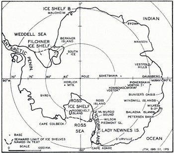
Fig. 1. Antarctica, showing places named in text

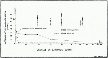
Fig. 2. Regime diagram of the ice sheet

The simplifications involved in Figure 2 are obvious. For example, to be fully useful in Section IV (p. 184), “the net balance of blown snow” should be separated into “snow blown in” and “snow blown out”, and the latter entered in the gross ablation total. But in broad outline the Figure is probably correct. The significant feature of it is that the area CDE is roughly 50 times the area ABC. In other words, assuming a mass budget in equilibrium, about 98 per cent of the accumulation on the grounded ice sheet reaches the sea, and remains to be ablated by it, either directly from the coastal ice cliffs or indirectly from the floating ice shelves. This conclusion agrees roughly with those of Reference MellorMellor (1959[b]) and Reference ListerLister (1959); the former concludes that roughly 10 per cent of the grounded ice sheet may be ablated before it reaches the sea; the latter thinks that ablation from the grounded ice sheet is not very significant at all. However, the strict quantitative accuracy of Figure 2 is not important. The main purpose of the Figure and the calculations above is to emphasize the overwhelming surplus in the budget of the grounded ice sheet. It appears now from both theory and movement studies that the Antarctic Ice Sheet is not, as it has so often been described, “static” or “sluggish” or “passive” but is in fact highly active. Indeed, its mean velocity around its periphery of roughly 15,000 km. must be of the order of hundreds of meters per year.

It will be noticed that Figure 2 does include an ablation zone. Such a zone is ice-covered only because it is supplied with ice from “up-stream”. As Avsyuk and others (Reference Avsyuk1956) have pointed out, the share of this supply entering any particular part of the ablation zone depends on the subglacial relief at the firn line. Relatively high parts of the ablation zone, especially if they are flanked by deep valleys, form the ice-free areas or “oases” such as Vestfold Hills, Bunger’s Oasis, the Windmill Islands and the mountains of south Victoria Land. However, over most of the periphery of Antarctica the supply of ice is great and the relief subdued, so that little of the ice is lost in the ablation zone and most of it reaches the sea.

(b) Ice cliffs and ice shelves

The line where the ice sheet begins to float will be referred to as “the grounding line”. Beyond this line the surplus of ice is exposed to the ablating influences of bottom melting and calving. Exactly what happens to the surplus depends on the thickness and velocity with which it reaches the coast and on the configuration of the coast and sea bed. For roughly half its margin the ice sheet terminates directly in the form of ice cliffs. Over the other half it pushes out to sea as a floating ice shelf. Eventually, even the ice shelves are limited by calving. This appears to be an extremely efficient ablating process and it is doubtful whether any ice shelf can exist beyond the limits of the relatively shallow continental shelf. This point has been developed by Reference SwithinbankSwithinbank (1955), who has shown how important to ice shelves are grounding points or anchors of rock at their seaward margins.

(a) The grounded ice sheet

The surface of the grounded ice sheet has a convex profile which is roughly similar from place to place. The profile illustrated in Figure 3 is that inland from “Mirnyy”, where most data are available; it has been drawn, as far as possible, along a line of maximum slope, using the American Geographical Society map of Antarctica, and the Soviet map which accompanies an article by Reference DolgushinDolgushin (1958). This and other profiles have been discussed by various authors, especially by Reference VyalovVyalov (1958). They are discussed briefly below, in the light of a recent paper by Reference NyeNye (1959), whose treatment is particularly suitable for use in Sections III and IV. Nye’s main conclusion is that, because the temperature of a polar ice sheet is highest at the base (due to geothermal and frictional heating) and because the plasticity of ice increases strongly with temperature, nearly all the “relative motion of the ice sheet, whether between ice and ice, or between ice and rock, is essentially concentrated at the bottom”. On this assumption he establishes the following law of sliding:

(1)

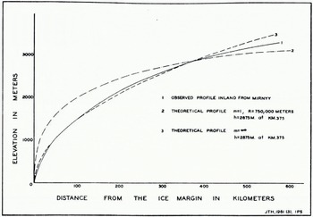
Fig. 3. Observed and theoretical profiler rf the ice sheet

and combines this equation with the following

(2)

(3)

to obtain a general expression for the profile of a circular (three-dimensional) ice sheet on a horizontal base:

(4)

where a = the accumulation rate, assumed uniform over the whole sheet, x = the distance from the center of the sheet, h = the thickness of the ice at any point, u = the horizontal velocity (assumed uniform with depth) of the ice at any point, τ = the shear stress at the bed, p = the density of the ice sheet, g = the acceleration due to gravity, α = the maximum surface slope at any point = −dh/dx(right-hand half of the ice sheet), R = the radius of the ice sheet, and A and m are constants, discussed below.

m, analogous to the exponent n in Glen’s flow law (equation (6)), is probably 4.2 (Reference GlenGlen, 1958) in the case of motion between ice and ice, which is probably the movement mechanism where the ice base is below freezing (see the theoretical discussion by Reference WeertmanWeertman (1957[a]) and field observations by Reference GoldthwaitGoldthwait (in press)); and 2 5 in the case of motion between ice and rock, which may be a major movement mechanism where the ice base is at the melting point (see Reference WeertmanWeertman’s (1957[a]) sliding model).

A ^−m , assumed uniform under the whole sheet, is a constant which allows fer the conditions at the bed, where motion takes place. It may be considered as a function of four other quantities, Z, Y, X and W, dependent on the roughness of the bed, the constitution and temperature of the ice, and on the wetness at the bed. Little is known about the effect of roughness; it is perhaps important only when the ice is at the melting point and sliding; then it may vary considerably with position but not with time (with which this paper is concerned). On the constitution of the ice, it is likely that the application of a roughly uniform shear stress for thousands of years over hundreds of kilometers produces near the bed a fairly uniform type of ice. For the purpose of this paper the most important variations in A ^−m are likely to be produced by changes in the temperature and wetness at the base, and these are discussed in Section III.

Equation (4) may be used to discuss briefly the observed profile of Figure 3. Unfortunately it is impossible to compare a curve derived from the equation directly with that of the figure, since the former has to be based on assumptions which are certainly not true: that the ice base is horizontal, Z, X and W are constant, and the accumulation is uniform. However, whereas curves for m = 1 and any reasonable value of R are all too elliptical and give a profile which is much too steep at the edge and too flat at the center (Fig. 3), by putting m = ∞ one can obtain a parabola

(5)

(when d is the distance from the edge of the ice sheet, and both d and h are expressed in meters), which fits almost exactly the observed profile as far as km. 375 (near “Pionerskaya”, Fig. 3). This parabola happens to be the profile of a perfectly plastic ice sheet with a yield stress of 1.0 bar (Reference NyeNye, 1952). That it fits so well is an argument for saying that m is relatively large, probably not less than 2.5. Because it is so simple, equation (5) is used in Section V for the reconstruction of former ice profiles. (Beyond km. 375 this theoretical parabola rises above the observed ice surface. This may be lower for a variety of reasons, of which the most likely is that, because m is in fact finite, the lower velocities needed near the center of the ice sheet can be produced by lower shear stresses. Moreover, these lower velocities are in fact very much lower, because the accumulation in the interior is so small.)

(b) Ice cliffs and shelves

Turning now to the margin of the grounded ice sheet, this normally reaches the sea and forms an ice cliff. The height of this cliff rarely exceeds 30 m. and it is presumably limited by mechanical factors (although the theory on this subject is still uncertain (Reference LoeweLoewe, 1955)). Therefore, even where the ice sheet has sufficient mass to push out into deep water, the total thickness of its margin can rarely, once it begins to float, exceed 200 m. or so. If the supply from the grounded ice sheet is initially thicker than 200 m. then the cliff will, unless it is maintained by extremely vigorous calving, spread out into a floating ice shelf, which may spread seaward for any distance between a fraction of a kilometer and hundreds of kilometers. The thickness of ice shelves has been discussed by Reference RobinRobin (1958), who has shown that “an approximate equilibrium thickness is maintained at a given locality” and that this thickness depends on, in order of importance, horizontal forces at the edges and grounding points and on the local temperature and accumulation. (The horizontal forces are the reason why large ice shelves are actually much thicker than 200 m. in their landward parts.) One would expect, from the magnitude m, that the thickness is only partly dependent on the amount or velocity of the supply from the grounded ice sheet. This supply must spread out quickly to the equilibrium thickness for the area offshore and its velocity must be transmitted to the whole shelf.

It can be seen now that for budgetary reasons the supply of ice on the grounded ice sheet is normally sufficient for it to reach the grounding line, but that for mechanical reasons the ice sheet cannot push beyond that line without being transformed into a floating ice shelf. It follows from this that the boundary of the grounded ice sheet is determined chiefly by the position of the grounding line and therefore by sea-level. The implications of this are the subject of Section V.

(a) Their chronology

Consider first in what direction the temperature changed in Antarctica during the glacial fluctuations of the Northern Hemisphere. The theoretical answer to this problem depends partly on the unknown causes of Pleistocene temperature fluctuations. If these causes affected the whole world evenly then Antarctic fluctuations were probably in phase with those of the Northern Hemisphere. If the causes were localized in the Northern Hemisphere, as in the theory of Reference Ewing and DonnEwing and Donn (1956), Antarctic fluctuations were again probably in phase, though perhaps diluted. On the other hand, according to Milankovitch’s well-known theory (reviewed by Reference FlintFlint ([1957], p. 508)) the causes of the fluctuations were not in phase in different hemispheres. However, wherever the causes of climatic change are localized, the atmospheric circulation works to spread their effects fairly uniformly over the whole globe; and Reference SimpsonSimpson (1940), for example, has argued that because of this the temperature fluctuations of different hemispheres are forced to be in phase.

This theoretical argument is supported now by a large amount of field evidence. In New Zealand, radiocarbon dating of the Otira Glaciation suggests that this was contemporary with the northern Würm (Weichsel, Wisconsin) Glaciation (Reference GageGage, 1961). In Antarctica itself four types of evidence suggest that a twentieth century warming there has paralleled that in the Northern Hemisphere.

• i. As part of the I.G.Y. program numerous snow pits and cores were dug and drilled in Antarctica, and these have yielded information on the climate for several hundred years past. Most of these investigations are still in progress; however, Reference GiovinettoGiovinetto (1960[b]) has reported at the South Pole thicker crusts which suggest warmer summers in the last 50 yr., and Cameron (personal communication) has reported at S-2, “Wilkes Station”, thickened ice layers which may suggest the same.

• ii. Reference MellorMellor (1960) has shown that a recent climatic warming provides the best explanation of a downward decrease of temperature measured in the upper 40 m. of the ice sheet south of Mawson.

• iii. In the same paper Mellor discusses air temperature changes actually measured by the Antarctic expeditions of the twentieth century. A similar discussion has been published by Reference WexlerWexler (1959). Both suggest a warming.

• iv. A recent thinning of the Antarctic Ice Sheet has been reported from at least three places: by Reference Hollin and CameronHollin and Cameron (1961) (snow patches at “Wilkes Station”), by Reference Yoshikawa and ToyaYoshikawa and Toya (1957) (snow patches at “Syowa”) and by Reference ShumskiyShumskiy (1959) (the ice sheet at Gaussberg). In the case of Gaussberg the thinning was determined by comparison with the records of the German South Polar Expedition of 1901–03, so that part at least of the thinning is definitely of this century.

(b) Their amplitude

The biggest temperature changes during the Pleistocene occurred in the neighborhood of the fluctuating ice sheets of Eurasia and North America, but away from these most evidence suggests that the temperature drop was smaller and roughly uniform. A survey of the problem by Reference FlintFlint (1957) suggests a world-wide drop of the order of 6° to 8° C. In the Southern Hemisphere, Reference WillettWillett (1950) has suggested that New Zealand at the Pleistocene temperature minimum was 6° C. colder than today. As for Antarctica itself, from Sections IV (p. 184) and V of this paper, the general configuration of the ice sheet there is fairly stable. It is probable, therefore, that the temperature drop there also may have been of the order of 6° C., and perhaps less than that in the center of the continent.

(a) Their effect on ice temperatures

The velocity of a cold ice sheet, and therefore its thickness, is dependent on the temperature of its lowest layers (Reference NyeNye, 1959). Therefore, consider how a drop of 6° C. at the surface of the Antarctic Ice Sheet would have affected its base. If the ice sheet were completely static, the vertical temperature profile in it would depend simply on the mean air temperature, the thermal diffusivity of ice and the geothermal heat flux, and would be linear. Pleistocene fluctuations of the mean air temperature would have been superposed on this profile in accordance with the equation for periodic heat flow:

(7)

If, in this equation, T _o , the range (amplitude×2) at the surface, is 6° C.; D, the distance below the surface, is 4,000 m.; Δ, the thermal diffusivity of glacial ice, is 15×10⁻³ cm.²/sec. (Reference Cameron and BullCameron and Bull, 1961) and P, the period, is 100,000 yr., then T_r , the range at the base, is negligible. In other words, the base of a static ice sheet would have been effectively insulated from the temperature changes at the surface.Footnote * In practice, however, the Antarctic Ice Sheet is not static, and the temperature distribution in it is modified by the downward and outward movement of the cold surface snow and by frictional heat generated near the hase. The effects of these “movement” factors have been considered by Reference RobinRobin (1955). In the context of this paper, which is concerned with temperature changes, it is clear that the downward movement of snow and ice must provide a cooling mechanism much more effective than the simple conduction evaluated above. A mathematical treatment of this movement cooling might be difficult; however, it follows from the argument on page 175 that each of the major Pleistocene temperature fluctuations lasted long enough for ice equal in volume to the ice sheet to have circulated through it several times over; therefore, it seems probable that movement cooling must have been able to transfer the 6° C. cooling of the surface to the major part of the ice base. The most vigorous circulation must have been through the upper and outer parts of the ice sheet but simple conduction must have completed the transfer through its long-traveled lowest layers.

Robin’s paper suggests one interesting reservation at this point. Robin showed that the smaller the accumulation is on an ice sheet then the smaller is the movement of cold into it and the greater the temperature difference that the geothermal flux can sustain between the base and the surface. For example, an ice sheet 3,000 m. thick with an accumulation of only 4 g./cm.² yr. should be 10° C. warmer at the base than one with twice that accumulation. It will he seen in Section IV that one possible result of a drop in air temperature might have been a drop in accumulation. In such a case the atmospheric cooling might have been completely offset by a decrease in the movement cooling.

(b) Their effect on velocity and thickness: the general case

With the reservation above, it appears that the greater part of the ire sheet was probably cooled by approximately 6° C. during each Pleistocene glacial stage in the Northern Hemisphere. These coolings must have caused at the ice base changes of temperature or wetness. which in turn must have produced changes in the value of A ^−m (see p. 177. It is now possible to proceed immediately to the main point of this section: that these changes have only a small effect on ice thickness. From equation (4)

(8)

i.e. h varies with only the minus one-ninth power of A ^−m in the case of a frozen base see p. 178 and the minus one-sixth power in the case of a melting base.Footnote † This result deserves a fuller explanation. If the ice at the base is cooled it becomes less plastic and the velocity of the ice sheet is reduced. To maintain the velocity needed to dispose of the accumulation an increased shear stress is required. However. since the velocity is dependent on a high power of the shear stress, this increase need not be large. Moreover, an increase in the shear stress involves an increase in thickness; any given column of the ice sheet contains more material. and consequently the velocity need not be maintained at its original value.

(c) Their effect on velocity and thickness: the Antarctic Ice Sheet

Equations (4) and (8) imply that A ^−m is uniform under the whole ice sheet, and that when this constant changes it changes everywhere by the same amount. In practice A ^−m is not uniform and during the Pleistocene it must have changed by different amounts in different parts of the Ice sheet. To determine these amounts and their actual effects on ice thickness. let us hest imagine three different ice sheets, each uniform at the base. but each distinguished try a different type elf base.

• i. Ice sheet 1. Imagine an ice sheet with its base currently below the freezing point. A cooling of 6° C. at the surface would cool the base by the same amount. In this ice sheet movement is purely by creep (see p. 178). It can be seen from equation (6) that a cooling of 6° C. would reduce the creep rate by a factor of roughly 2, and, by analogy with equation (1), this would act as a reduction in A^−m . Since the thickness of ice sheet I would be dependent on the minus one-ninth power of A^−m , it would increase by a factor of

  
  i.e. 1.08. This result is of general interest; it implies that the thickness of any icc sheet which is frozen to its base is very insensitive to temperature changes, particularly in view of the thermal restraints discussed on page 183.

• ii. Ice sheet 2. Imagine an ice sheet with its base currently at the melting point and with a small heat surplus available for basal melting. A cooling of 6° C. at the surface would freeze the base and cool it to between 0° and −6° C. Now, the mechanical behavior of ice close to the freezing point is not well known, and it is necessary to draw on a purely theoretical treatment by Reference SteinemannSteinemann (1958). (Steinemann’s treatment concerns the reverse case to ours: a change from freezing to melting.) He argues that up to the melting point a temperature dependence of the Glen type applies (equation (6)). As soon as the melting point is reached additional heating by strain-work produces an increased soaking of the ice. In the case of a glacier the bottom 1 m. or so fills with water up to a volume fraction of 0.15, at which point the water-filled pores interconnect and further melt water is pressed out and flows as free melt water. This soaking of the ice is accompanied, according to Steinemann, by an increase in plasticity much greater than that caused by any reasonable temperature changes below the melting point. He calculates, for example, for a shear stress of 1.0 bar, that the “wet” strain rate of “warm” ice is 15 times greater than the “dry” strain rate. Also, as the melting point is reached, movement mechanisms other than pure creep may develop. The “sliding” suggestion by Reference WeertmanWeertman (1957[a]) may be such a mechanism. It is difficult to predict how such mechanisms would affect the factor of 15 given above, but they are likely to increase it. Thus, in ice sheet 2, a cooling would reduce A ^−m at least 15 times, and this would produce, from equation (8), an increase in ice thickness by at least 1.6 times. This is a large increase, but there is some field evidence that changes of this magnitude would occur, An increase of thickness by a factor of 1.6 involves an increase in surface slope by 1.6 and an increase in the basal shear stress by 2.6. Several workers have pointed out that shear stress differences of this order are probably associated with temperature or wetness differences at the ice base.

• iii. Ice sheet 3. Imagine an ice sheet with its base currently at the melting point, with a large heat surplus available for basal melting. A cooling of 6° C. at the surface would merely reduce the amount of melt water produced. This might affect the velocity of the ice. However, once a warm ice base reaches the stage where water is being pressed out of it, then both creep and sliding mechanisms may have reached their maximum efficiency. Further melt water may only be squeezed out into a basal film, or, more probably, into subglacial channels. It is unlikely that these have any further “lubricating” effect. However, even if this assumption here is incorrect and wetness changes do produce velocity changes, these would still affect the thickness only to the minus one sixth or so power.

• iv. The Antarctic Ice Sheet. In summary, the base of the Antarctic Ice Sheet is probably divided into “patches” of three types, corresponding to the three imaginary ice sheets discussed above. The thickness changes in patches of types 1 and 3 were probably small, but in patches of type 2 they may have been large. Therefore, it is unfortunate that the geographical distribution and area of these patches are largely unknown, and are likely to remain so until a great deal of drilling and calculation have been carried out. For the purpose of calculating a Würm volume change for Section VII it has been assumed, which is probably reasonable, that patches of type 2 are scattered over a total of one-third of the ice sheet; but that only half of these patches would in practice be frozen by a cooling—this is because of the thermal restraints discussed below.

(a) Meteorological arguments

The first effects of a cooling were probably a reduction in the amount of water vapor that the air above Antarctica could hold and a consequent reduction in accumulation. Of other possible effects, the most important must have been caused by changes in the vigor and pattern of the atmospheric circulation. Possibly the cooling reduced the vigor but, since the general configuration of the ice sheet is fairly stable (see p. 184 and 192), the pattern probably changed little. An analysis of all these effects was made in 1928 by Meinardus (reviewed by Reference SimpsonSimpson (1940)), whose calculations should be re-examined in the light of the now greatly increased meteorological data from Antarctica. For the reasons discussed on page 186, Meinardus was interested in the effect on accumulation of a warming of Antarctica. He found that an increase of temperature by 5° C. and of the wind velocity by 24 per cent would have combined to increase the outflow of ice by a factor of 2. One might expect then that a cooling by 6° C. with no major change in the wind would have reduced accumulation but by a factor of less than 2. A more precise result is not needed for this paper.

(b) Field evidence

Such as it is, the field evidence confirms this result. The pit and core studies mentioned on page 180 have provided records of the accumulation in Antarctica for the last several hundred years. From that section, Antarctic temperatures during this period have probably risen by the order of 1° C., from the eighteenth and nineteenth centuries climax of the Little Ice Age to the relative warmth of the twentieth century. However, no comparable increase in accumulation seems to have occurred. At “Wilkes Station” (S-2) there has been no major change in the accumulation since A.D. 1783 (Reference CameronCameron and others, (1959). At the South Pole there has been no major change since a.d. 1530, apart from a minor twentieth century increase with a maximum in the 1920’s (Reference GiovinettoGiovinetto, 1960[a], Reference Giovinetto[b]). (This increase correlates well with one recorded at “South Ice” (Reference ListerLister, 1959), which Reference LambLamb (1959) thinks may be related to a world-wide intensification of the circulation.) At “Byrd Station” the accumulation has actually decreased very slightly since A.D. 1547 (Reference Bender and GowBender and Gow, 1961).

(a) The effect in the “oases”

If ever the Pleistocene values of ablation and accumulation are determined more precisely, it will be useful to plot them as additional curves on Figure 2. Meanwhile, it seems from Figure 2 that, even after a two-fold decrease in accumulation, the total budget of the grounded ice sheet would have remained strongly positive, and that the greater part of the accumulation inland would have continued to reach the sea. There may have remained, in the higher parts of a narrow ablation zone, some small ice-free areas like those of today, where the boundary of the ice sheet may have changed slightly in response to the changes in ablation and accumulation. However, even if these changes were determined it would be very difficult to calculate the new boundary, for the following reasons. The effect of the ablation change might be assessed fairly accurately. The “accumulation” changes in the “oases” depend not only on the precipitation but also on what enters them as ice flow. To calculate the change in ice flow would require both a knowledge of the changed accumulation in the interior and an almost impossibly accurate knowledge of the subglacial relief there. Therefore, it will be even more difficult to reverse this procedure and to deduce from glacial geological evidence in the “oases” what were the changes in climate. Moreover, as will be seen in Section V, the limits of the ice sheet in the “oases” are in most cases practically independent of direct climatic control.

(b) The effect on the area and volume of the ice cover

It was noted on page 179 that, no matter what the supply of ice is on the grounded ice sheet, its limits (outside the few “oases”) and therefore its area can be changed only by changes in sea-level. Also, from page 177,the peripheral ice shelves are unlikely to spread beyond the continental shelf. Concerning the volume of the ice, although it was decided above that accumulation on the ice sheet may have been reduced by as much as a factor of 2, this does not mean that its thickness and volume were changed by a similar factor. As with temperature changes, the effect of (uniform) accumulation changes on the volume of the ice sheet can be estimated from equation (4), from which

(9)

a dependence suggested earlier by Reference NyeNye (1959). Assuming m = 2.5, a reduction of accumulation by 2 would have reduced the ice sheet only to (1/2)^1/6, i.e. to 90 per cent of its original height. Some of this reduction might have been offset by an increase in precipitation on the center of the ice sheet as it dropped towards the new level.

(c) Summary

When the Antarctic Ice Sheet first formed cannot be discussed in this paper; this question may be solved by oceanographic work. Some authors appear to favor a Tertiary rather than a Pleistocene beginning. However, it is probable from the discussion on page 176 and above that once the ice sheet was formed it was never afterwards ablated away, at least by any of the climatic conditions of the Pleistocene. Also, it seems unlikely to be ablated away in the foreseeable future. It may be argued that conditions were periodically sufficient to ablate away the northern ice sheets; but those ice sheets ended chiefly on land, and the ablation at their edges must have been considerable, even as they grew. But in Antarctica there is no such intense ablation; as has been seen, only the surrounding sea is effective in this respect.

(a) Eustatic and isostatic changes

A study of world-wide sea-level changes has been published recently by Fairbridge (1961). It appears from this that the sea-level in the past is unlikely to have been more than 100 m. (possibly 150 m.; see below) below that in the present, at least since the Cretaceous. If this is so, then Voronov’s apparent lowering of 300–500 m., if it occurred, cannot be explained ecstatically but only isostatically in terms of a relatively higher continental edge. Such might have been the situation at the climax of the first glaciation of the continent, perhaps for a few thousand years until the continental shelf sank under the weight of ice to the low level it has maintained probably ever since. Once the continental shelf sank to this level the subsequent position of the grounding line was presumably governed by sea-levels which apparently oscillated during the Pleistocene between highs in the northern interglacials and lows in the glacials. According to Fairbridge the lows became progressively lower until that in the Würm. Recent evidence by Reference EwingEwing and others (1960) suggests that this Würm depression was roughly 150 m., and this value is used in Figure 4 and on page 189.

(b) Relative change by ice shelf thickening

An additional relative lowering of sea-level may have been produced by a thickening of the ice shelves as a result of the lower temperatures associated with the northern glacial stages. This thickening can be investigated quantitatively. Reference WeertmanWeertman (1957[b]) has established the following equation for the creep rate, K, of an ice shelf free to expand along the vertical and one horizontal axis:

(10)

where ρ_I and ρ_W are the densities of ice and sea-water, g is the acceleration due to gravity, H is the thickness of the shelf, and n is probably 4.2 (see p. 178). A is a constant analogous to that on page 178 and may, from there and from equation (6), be considered as the product of a constitution constant and a temperature constant exp(Q/RTn).

For K substitute a/H, where a is the accumulation rate. Equation (10) can then be solved for H in terms of T or, for interest, a. The integral is awkward; A depends on T, but T is hard to estimate (and is affected, incidentally, by a, by the Robin movement effect) and its distribution is dependent on the unknown H. However, consider temporarily the unreal case of a homogeneous, isothermal ice shelf. In that case the integral reduces to AH, and the following solutions are obtained:

(11),(12)

If equation (12) is evaluated for isothermal shelves at 0° and –30° C., H changes by only 2. Since the temperature spreads in modern ice shelves (and presumably in Pleistocene ones) are only a fraction of the above (for example, all shelves have approximately the same bottom temperature), it is clear that their thicknesses cannot be strongly dependent on temperature.

As a matter of interest this result draws attention to the problem of why, for example, parts of Maudheim Ice Shelf B (Reference RobinRobin, 1958) should be only 250 m. thick while the greater part of the Ross Ice Shelf is 350 m. thick (Reference CraryCrary, 1959). It appears from the above that differences in temperature and accumulation (note that this has to include bottom freezing or melting) are unlikely to account for all of this difference, especially since their effects in this case are probably in opposite directions. Now, inspection of Weertman’s paper suggests another factor which might well be included in Robin’s “horizontal forces”. In addition to equation (10) above, Weertman derived an equation for the creep rate, K ₁,of an ice shelf free to expand along the vertical and both horizontal axes. K ₁ ≈ 1.1 K. Now K ₁ equals not a/H ₁ but a/2H ₁(cf. Reference NyeNye’s (1959) two- and three-dimensional ice sheets). Solving both of Weertman’s equations (for homogeneous, isothermal shelves) it is found that H ₁ equals only 0.86 H. H ₁ probably applies to the outer part of the Maudhcim shelf, but H to the Ross Ice Shelf, constrained between Ross and Roosevelt Islands. Indeed, since the Ross Ice Shelf is not merely channeled but actually squeezed between these islands, the ratio of H ₁ to H may be even less.

(a) At the edge of the ice sheet

It appears then that during the Würm Glaciation the grounding line in Antarctica was 150 m. lower than it is today, chiefly because of the eustatic effect. As a result, the main grounded ice sheet advanced by a distance which depended on the angle of the sea floor. From Reference LawLaw (1961) and assuming that the sea is 200 m. deep at the present ice edge, this angle averages, very roughly, 0.1°. This would have produced an average advance of 90 km. These values are used in Figure 4. Now, it appears from Figure 4 that, because of the profile of an ice sheet, such a sheet need advance only a very small distance before its old margin is covered with a very great thickness of ice. Thus, the above-mentioned advance of 90 km. may seem small (only 4 per cent of the present radius of the ice sheet), but it would have been enough to thicken the present ice margin by 1,230 m. This is more than enough to account. for example, for the frequently-quoted previous glaciation of Gaussbcrg (373 m. high). In some cases, as was seen on page 186, a flatter sea floor, such as that beneath the Ross Ice Shelf, would have produced an advance of as much as 500 km. This in its turn would have produced an increase in ice thickness (subject to limitations discussed later in this section) of roughly 3,000 m. Clearly the history of each part of the Antarctic periphery needs to be considered in the light of its own submarine topography.

(b) An isostatic restraint

The hypothetical advances discussed above might have been reduced considerably by isostatic effects. Consider a point at the ice margin where, by a combination of a 150 m. sea-level drop and the sea-floor angle, an advance of t 3.5 km. took place. From equation (5) the additional thickness of the ice sheet at its old margin would be 545 m., which, if isostatic compensation were locally perfect, would depress the rock beneath by 545 m. multiplied by the density of ice and divided by the density of the mantle; that is by 150 m.; which would completely counteract the effect of the eustatic drop. In practice such perfect compensation is not realized, for a number of reasons. First, since the compensation is spread over a wide area, the average additional thickness rather than that at one point should be considered. Secondly, compensation is rarely complete, because the shear strength of the crust is considera-able. Indeed, at first sight it seems unlikely that a disturbance only 90 km. across should have any isostatic effect at all. However, since the other dimension of this disturbance is essentially 15,000 km. (the circumference of the continent) a limited adjustment might be expected. Thirdly, there is a time lag between loading and compensation, although this should be small compared with the periodicity of the fluctuations.

At present, after the Würm Glaciation, it is possible to study this isostatic restraint in the reverse direction only: as the rebound of the land reduces the relative post-glacial rise of sea-level. Evidence for the rebound is provided by the raised beaches reported from every coastal location in Antarctica, and possibly by the coastal gravity deficiency reported by Reference Ushakov and LazarevUshakov and Lazarev (1959). Evidence for its limited amplitude is provided by the fact that the maximum elevation of these beaches is everywhere measured in tens of meters rather than in hundreds, as in Europe and North America.

(c) At the center of the ice sheet

It will be noticed on Figure 4 that the increase in ice thickness produced by an advance becomes much less as one goes inland. This is a point which has been overlooked by several authors who, for example, have taken the evidence that the ice in Victoria Land was once 1,200 m. thicker to mean that the ice over the whole continent was that much thicker. This has led them to overestimate the volume of additional ice involved in glacial maxima. It appears from this section and from Sections III and IV that, once it was established there, the ice in central Antarctica did not fluctuate in thickness by any appreciable amount at all. A confirmation of this argument is provided by the preliminary gravity results from Antarctica: approximate isostatic equilibrium has been reported for both West Antarctica (Reference BentleyBentley and others, 1960) and East Antarctica (Reference SorokhtinSorokhtin and others, 1960). In view of what is now known of the structure of Antarctica, the negative Bouguer anomaly reported along the route of the Commonwealth Trans-Antarctic Expedition (Reference PrattPratt, 1959) is perhaps best interpreted as a normal continental rather than isostatic effect.

(a) The coastal “oases”

It follows from this section that the ice margin in an “oasis” may be determined not so much by climatic factors as by the need for the margin to be in mechanical equilibrium with surrounding glaciers whose limit is determined by sea-level. This point is illustrated below by a simplified treatment of some aspects of the glacial geology of the Windmill Islands, of which a map and general description have been published by Reference Hollin and CameronHollin and Cameron (1961). (Climatic factors were not completely unimportant in the glacial history of the Windmill Islands; the author hopes to discuss their effects in a future paper; but they were almost certainly overshadowed by the sea-level effect.)

• i. The Windmill Islands and peninsulas are currently ice-free chiefly because they are relatively high, so that the ice sheet inland from them drains more easily via the lower areas to the south-west and north-east, where its limit is determined by sea-level. To the north of the Windmill Islands the sea is extremely shallow (the Petersen Bank) and when the sea-level was lowered during the Würm Glaciation the ice sheet probably advanced across this bank for several tens of kilometers (p. 186). From equation (5) the ice must have been of the order of 1,000 m. thick in the neighborhood of the present Balaena Islands: a height it could not have maintained without covering the Windmill Islands to the south.

• ii. Conversely, at the end of the Würm Glaciation the deglaciation of the Windmill Islands was probably governed not so much by the climatic improvement as by the post-glacial rise of sea-level. Probably this rise began about 18,000 yr. b.p. and probably the retreat of the Antarctic Ice Sheet began at about the same time, From Reference FairbridgeFairbridge (1961), the main rise was not completed, however, until about 6,000 yr. b.p., which, ignoring various time lags, must have been the date at which the ice sheet assumed the general configuration it has today. Subsequent modifications to this were provided by the “ablating down” process (see p. 175) and by isostatic rebound.

• iii. It follows from the above that if the deglaciation process was still continuing as recently as 6,000 yr. b.p., then shells, whalebone, etc. from the subsequent raised beaches will tend to be younger than those from Northern Hemisphere beaches, whose emergence was governed more directly by climatic factors. In fact, all the Antarctic radiocarbon dates known to the author do post-date 6,000 yr. B.P. Clearly these low ages should not be mistaken for evidence (see p. 186 and 193) that the deglaciation of Antarctica has been produced by an accumulation decrease following the Climatic Optimum. If the search areas are chosen carefully, it should be possible to find in Antarctica post-glacial material as old as any in the Northern Hemisphere. Promising areas would be bird rookeries on high nunataks, where a useful dating material might be the thick, durable layers of oily “bird-spittle”. (The author is grateful to A. Heine of the New Zealand Geological Survey for drawing his attention to this material.)

• iv. Frequently, in the Windmill Islands and elsewhere (Reference Hollin and CameronHollin and Cameron, 1961), current ice cliffs abut against islands and peninsulas possessing undisturbed sequences of raised beaches. This argues strongly for, although it does not prove, a current advance of the ice. Originally this advance was thought by the author to be a mass budgetary phenomenon, possibly related to the Little Ice Age of the Northern Hemisphere but with a lag due to the size of Antarctica. Now, however, it seems more likely that the advance is a secondary effect of the isostatic rebound that produced the raised beaches; the rebound had the effect of relatively lowering sea-level; the budgetary and mechanical limit of the sea was removed; and the ice sheet moved forward a little.

(b) The Ross Sea area

It was seen on page 187 that a fall in sea-level of 150 m. would ground the eastern half of the Ross Ice Shell. Such a grounding would eliminate the ablation by bottom melting which probably occurs there, and a colder and shallower Ross Sea to the north would probably be capable of less calving action.at the shelf edge. On budgetary grounds, therefore, there is a strong possibility that the shelf would advance northwards towards the edge of the continental shelf (roughly a line between Capes Adare and Colbeck). As it advanced it would ground on the large and numerous banks, with a depth of less than 200 fathoms (366 m.), on the Ross Sea floor (see U.S. Navy Hydrographie Office Chart No. 6636). Where it grounded one would expect to find “ice hills” (Reference RobinRobin, 1958), similar to the present Roosevelt Island, with roughly parabolic profiles. Possibly, the horizontal forces at these ice hills would be sufficient (as in West Antarctica; see p. 185) to ground the shelf even where the water is relatively deep. On this question one can refer to the parallel case of the Filchner Ice Shelf: a large area of that shelf manages to float inland from Berkner Island, but it is over 600 m. thick, which means that it would be well grounded if it were in a Ross Sea 150 m. lower than today. In theory, it appears that a general grounding of the Ross Ice Shelf could have taken place, particularly at the beginning of the Antarctic glaciation and during the Würm; in practice, however, the isostatic restraint could have restricted this grounding to the banks. The history of the Ross Sea may be contained in its sediments and recent investigations of these have been made by Reference ThomasThomas (1960). (Thomas claims that there has been no ice shelf in McMurdo Sound for 33,000 yr.; this author feels that a more adequate dating is needed to justify this conclusion.)

Consider some probable effects of a grounding of the Ross Ice Shelf. First, the appearance of the area would be different; horizontal surfaces would be replaced by convex ones which would rise steeply to one, two or three thousand meters. Secondly, the “dry valleys” of Victoria Land would be filled not so much by the frequently postulated “ice floods” from the interior to the west (though such may have occurred) as by the intrusion of ice lobes from the grounded shelf to the east.Footnote * Thirdly, at its greatest development a Ross Ice Sheet might deflect from West Antarctica warm, moist air which today reaches it, and inhibit the katabatic winds which arc responsible for the currently great ablation in the dry valleys. Finally, with a warming climate and rising sea-level, one might expect the retreating ice sheet and ice shell to leave behind it relict masses of ice, some of them stranded by isostatic rebound. Various workers have suggested that the Lady Newnes Ice Shelf and the Wilson Piedmont Glacier originated as such relicts.