


Introduction
Process-based crop models are commonly used to simulate growth, development, yield and other characteristics of field crops as well as related soil processes such as the soil, water and nitrogen balances. These models simulate such interconnected soil–plant–atmosphere system that is influenced by agronomic practices (e.g. Ritchie, Reference Ritchie1981; Jones et al., Reference Jones, Hoogenboom, Porter, Boote, Batchelor, Hunt, Wilkens, Singh, Gijsman and Ritchie2003). The use of different crop models for assessing possible future climate change impacts, including analyses oriented to derive adaptation strategies, is increasing (Corbeels et al., Reference Corbeels, Berre, Rusinamhodzi and Lopez-ridaura2018; Rötter et al., Reference Rötter, Appiah, Fichtler, Kersebaum, Trnka and Ho2018). Due to the nature of modelling, there is always a certain degree of uncertainty (e.g. due to the need for certain simplification against the real system) within results which may raise doubts about the reliability of the results (Rötter et al., Reference Rötter, Carter, Olesen and Porter2011). The use of crop model ensembles (against only one model with its specifics) is among the recommended approaches (Martre et al., Reference Martre, Wallach, Asseng, Ewert, Jones, Rötter, Boote, Ruane, Thorburn, Cammarano, Hatfield, Rosenzweig, Aggarwal, Angulo, Basso, Bertuzzi, Biernath, Brisson, Challinor, Doltra, Gayler, Goldberg, Grant, Heng, Hooker, Hunt, Ingwersen, Izaurralde, Kersebaum, Müller, Kumar, Nendel, o'Leary, Olesen, Osborne, Palosuo, Priesack, Ripoche, Semenov, Shcherbak, Steduto, Stöckle, Stratonovitch, Streck, Supit, Tao, Travasso, Waha, White and Wolf2015; Wallach et al., Reference Wallach, Mearns, Ruane, Rötter and Asseng2016) enabling estimation of the range of outputs, leading to more robust predictions and the possibility of reducing uncertainties. Several studies that applied model ensembles across different conditions have shown that the ensemble median (EnsMED) or mean (EnsAVG) provide more robust assessments than individual models (e.g. Rötter et al., Reference Rötter, Palosuo, Christian, Angulo, Bindi, Ewert, Ferrise, Hlavinka, Moriondo, Nendel and Olesen2012; Asseng et al., Reference Asseng, Ewert, Rosenzweig, Jones, Hatfield, Ruane, Boote, Thorburn, Rötter, Cammarano, Brisson, Basso, Martre, Aggarwal, Angulo, Bertuzzi, Biernath, Challinor, Doltra, Gayler, Goldberg, Grant, Heng, Hooker, Hunt, Ingwersen, Izaurralde, Kersebaum, Müller, Naresh Kumar, Nendel, O'Leary, Olesen, Osborne, Palosuo, Priesack, Ripoche, Semenov, Shcherbak, Steduto, Stöckle, Stratonovitch, Streck, Supit, Tao, Travasso, Waha, Wallach, White, Williams and Wolf2013). Simultaneously, compliance of individual models can be shown from ensemble simulations in relation to monitored variables (e.g. Palosuo et al., Reference Palosuo, Kersebaum, Angulo, Hlavinka, Moriondo, Olesen, Patil, Ruget, Rumbaur, Takac, Trnka, Bindi, Caldag, Ewert, Ferrise, Mirschel, Saylan, Siska and Rötter2011). Usually, model ensembles were tested only for one individual crop, for example, the ensemble of 23 corn models presented by Bassu et al. (Reference Bassu, Brisson, Durand, Boote, Lizaso, Jones, Rosenzweig, Ruane, Adam, Baron, Basso, Biernath, Boogaard, Conijn, Corbeels, Deryng, De Sanctis, Gayler, Grassini, Hatfield, Hoek, Izaurralde, Jongschaap, Kemanian, Kersebaum, Kim, Kumar, Makowski, Müller, Nendel, Priesack, Pravia, Sau, Shcherbak, Tao, Teixeira, Timlin and Waha2014), the ensemble of eight models for winter wheat by Palosuo et al. (Reference Palosuo, Kersebaum, Angulo, Hlavinka, Moriondo, Olesen, Patil, Ruget, Rumbaur, Takac, Trnka, Bindi, Caldag, Ewert, Ferrise, Mirschel, Saylan, Siska and Rötter2011) or the ensemble of 11 models for spring barley (Salo et al., Reference Salo, Palosuo, Kersebaum, Nendel, Angulo, Ewert, Bindi, Calanca, Klein, Moriondo, Ferrise, Olesen, Patil, Ruget, Takáč, Hlavinka, Trnka and Rötter2016). The focus on individual crops separately is due to the fact that ensemble modelling is a technical and time-demanding procedure concerning data availability, technical aspects and personnel requirements. On the other hand, model ensemble evaluation focused simultaneously on several crops, is desired as the first step to enable simulating crop sequences and crop rotations by an ensemble approach. The simulations of crop sequences or rotations are closer to real-world conditions, with higher relevance of results (Kollas et al., Reference Kollas, Kersebaum, Nendel, Manevski, Müller, Palosuo, Armas-Herrera, Beaudoin, Bindi, Charfeddine, Conradt, Constantin, Eitzinger, Ewert, Ferrise, Gaiser, De Cortazar-Atauri, Giglio, Hlavinka, Hoffmann, Hoffmann, Launay, Manderscheid, Mary, Mirschel, Moriondo, Olesen, Öztürk, Pacholski, Ripoche-Wachter, Roggero, Roncossek, Rötter, Ruget, Sharif, Trnka, Ventrella, Waha, Wegehenkel, Weigel and Wu2015), because carry-over effects between seasons can be considered. At the same time, the long-term effects of weather, cultivated crops and agronomic management on soil properties can be assessed (Kersebaum, Reference Kersebaum2007; Hlavinka et al., Reference Hlavinka, Trnka, Kersebaum, Čermák, Pohanková, Orság, Pokorný, Fischer, Brtnický and Žalud2014), or climate change adaptation options can be tested (Hlavinka et al., Reference Hlavinka, Kersebaum, Dubrovský, Fischer, Pohanková, Balek, Žalud and Trnka2015). However, there is generally lower availability of data for model calibration from uninterrupted observations within crop rotation experiments. To cover the sufficient number of samples of each individual crop (or certain cultivars) of rotations, this could be alternatively solved through the data from individual crops experiments under defined conditions, which was applied in the current study.
The current paper focuses on simultaneous modelling of four separate crops (winter wheat, spring barley, silage maize and winter oilseed rape) based on field experiments with comparable methodology and compares 13 crop growth models. These comparisons were made under contrasting climatic conditions represented by three different sites in Central Europe. The main objective of the current study was to identify potentially best-performing models and to compare them with the ensemble approach, which could be used, for example, for impact and adaptation measures assessment studies both under present and expected climatic conditions. The present study is an essential first step for selecting the most proper models that would be suitable for modelling uninterrupted crop sequences or rotations by ensemble or individual models.
Materials and methods
Models
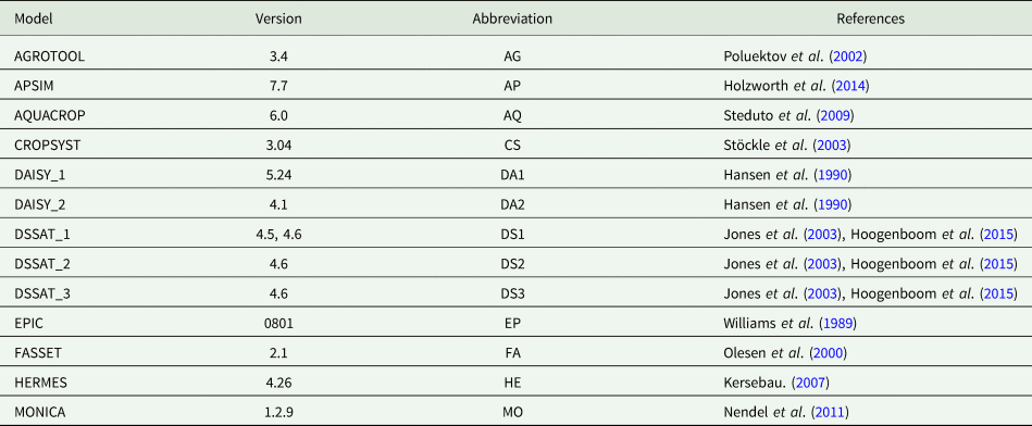
The current study included 13 crop growth models varying in complexity and functionality. Concurrently, two models were operated by different users and were independently evaluated. The DAISY model was operated by two independent modelling groups (marked as DAISY_1 and DAISY_2) and the DSSAT model was operated by three independent modelling groups (marked as DSSAT_1, DSSAT_2 and DSSAT_3). Specifically, 28 modellers from 10 countries participated in the study. The models that were used and their appropriate references are listed in Table 1, and the major characteristics of the participating models are summarized in Table 2.
Table 1. List of models, their abbreviations used in the current study and references
In the case of DAISY_1 and DAISY_2, the same model was used, but the simulations were performed by two different modelling teams. Analogously, in the case of DSSAT_1 (v4.5: spring barley, winter wheat, silage maize, v4.6 winter oilseed rape), DSSAT_2 and DSSAT_3, the simulations were performed by three separate teams.
Table 2. Parameters and modelling approaches of the included models

a Leaf area development and light interception: S – simple or D – detailed approach.
b Light utilization/biomass growth: RUE (simple approach) – Radiation use efficiency, P-R (detailed approach) – Gross photosynthesis minus respiration, and TE – transpiration efficiency biomass growth.
c Crop phenology is a function of T – temperature, DL – photoperiod (day length), V – vernalization, and O – other water (nutrient) stress effect considered.
d Yield formation depending on HI – harvest index, B – total (above-ground) biomass, Gn – number of grains, and Prt – partitioning during reproductive stages.
e Water dynamics approach (app.): C – capacity app. and R – Richards app.
f Evapo-transpiration estimation methods: P – Penman, PM – Penman-Monteith, PT – Priestley-Taylor, Mak – Makking, and mPM – modified Penman-Monteith.
g Soil CN model, C – C model, N – N model, P(x) – x = organic matter pools number, and B – microbial biomass.
Experimental sites and crop selection
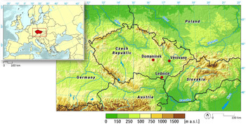
The test sites selected in the current study (spatial locations in Fig. 1) represent substantial temperature and precipitation gradients for winter wheat, spring barley, silage maize and winter oilseed rape cultivation within the Czech Republic, and the sites are also representative of wider Central European conditions. The Lednice experimental site represents a warm and relatively dry region, Věrovany is a production area with a fertile soil, where warm and mostly sufficient rainy conditions prevail and Domanínek is characterized as a colder and wetter production area (Table 3).

Fig. 1. Right: The Czech Republic within Europe (in red). Left: Locations of the Lednice, Věrovany and Domanínek experimental sites in the Czech Republic.
Table 3. Experimental sites' characteristics (the reference period for the average annual temperature and precipitation is 1981–2010)

Selected crops represent more than 0.6 of arable land in the Czech Republic and are crucial also within neighbouring countries. Winter wheat (variety Samanta), spring barley (variety Tolar), silage maize (variety Cefran in Lednice and Věrovany and variety Cingaro in Domanínek) and winter oilseed rape (variety Artus) were selected as representative varieties for each experimental site:
• Samanta (registration 2006) ranks among the semi-early winter wheat varieties with medium-grain and medium tillering. Resistance to overwintering and tolerance to late sowing are advantages of this variety.
• Spring barley variety Tolar (registration 1997) represents the semi-early malting variety preferred by malt-houses to produce Czech beer. For the warmer production area, Tolar has moderately high grain yield. The plants have medium to high heights and medium resistance to lodging (CISTA 2007).
• The Cefran variety (registration 2003) is a medium-late maize hybrid suitable for silage within the warm production area. The high yield and starch content in total dry matter are an advantage of Cefran (CISTA 2004). The variety Cingaro (registration 2006) is among the very early hybrids achieving above-average dry matter yield. Cingaro is resistant to cold weather, and its fibre is well digestible (Dobos, Reference Dobos2004).
• The Artus variety (registration 1999) of winter oilseed rape is a medium early hybrid variety. Plant height is medium to high, which causes the crop to have low to medium resistance to lodging. It tolerates overwintering and is characterized by high grain yield and very low glucosinolate content (CISTA 2006).
Model calibration and criteria for evaluation
The results of models and their ensemble were evaluated on the basis of acquired available data sets from rainfed variety trials conducted by the Central Institute for Supervising and Testing in Agriculture (CISTA). Data from the period 1991 to 2010 for the three selected experimental sites and for each crop (winter wheat, spring barley, silage maize and winter oilseed rape) were used. There was the comparable experimental protocol along all sites. Moreover, constant cultivars of selected crops were included throughout the whole period, so the technological trend did not have to be considered. The observed experimental data that were available included the dates of sowing and harvest, amounts of seeds sown per m2, observed phenological phases (emergence, tillering, shooting, heading, flowering and maturity), the number of tillers per m2, the weight of 1000 seeds, fertilizer application data (timing and amount fully representing real field experiment management) and information on the previous crop. Additionally, the information about texture, bulk density, total pores, hydrolimits (field capacity, wilting point), the content of organic carbon, total nitrogen and pH for defined layers of included soil profiles (one specific soil profile for each station) were available. Not known from the trials was information on tillage and was thus not available to the modellers. Initial conditions for the available soil water (% volumetric) at depths of 0.0–0.4 and 0.4–1.5 m and soil mineral nitrogen contents (kg N/ha) at depths 0.0–0.4 and 0.0–0.8 m were set. For winter oilseed rape, the initial conditions were defined on 1 August, for winter wheat 1 September, for spring barley and silage maize 1 November of each year (constant dates within the years for individual crops). As soil moisture was not observed, the SoilClim model (Hlavinka et al., Reference Hlavinka, Trnka, Balek, Semerádová, Hayes, Svoboda, Eitzinger, Možný, Fischer, Hunt and Žalud2011) was used to estimate soil water content at the beginning of each simulation based on preceding meteorological conditions. Further, the observed initial soil mineral nitrogen content was not available. It was alternatively estimated from the average of the measured amounts at each of included sites and from parallel CISTA field experiments focused on nitrogen balance, ranging from 85 to 140 kg of mineral N in the soil per hectare. The sowing dates within the database differed from year to year according to the suitability of the current weather conditions and soil moisture. The mean date of sowing was on 28 August for winter oilseed rape, on 2 October for winter wheat, on 3 April for spring barley and 30 April for silage maize.
The concept of the study was not in the form of a classical division into a calibration part of the database and a subsequent validation on an independent data sample. Rather only a minimal calibration concept was adopted with subsequent evaluation of results based on the whole data set (without independent data sample). This approach was used due to the absence of more detailed observations (such as the development of aboveground biomass, leaf area, nitrogen content in biomass, measured initial soil conditions before sowing, etc.), which would be required for a detailed calibration (Kersebaum et al., Reference Kersebaum, Boote, Jorgenson, Nendel, Bindi, Frühauf, Gaiser, Hoogenboom, Kollas, Olesen, Rötter, Ruget, Thorburn, Trnka and Wegehenkel2015). This mimics the typical situation of a regional parameter adjustment and assumed, that models were already parameterized for the specific crop and require only a minimum adjustment to reflect the regional varieties. This procedure was already applied by several model ensemble studies on climate change impacts (e.g. Asseng et al., Reference Asseng, Ewert, Rosenzweig, Jones, Hatfield, Ruane, Boote, Thorburn, Rötter, Cammarano, Brisson, Basso, Martre, Aggarwal, Angulo, Bertuzzi, Biernath, Challinor, Doltra, Gayler, Goldberg, Grant, Heng, Hooker, Hunt, Ingwersen, Izaurralde, Kersebaum, Müller, Naresh Kumar, Nendel, O'Leary, Olesen, Osborne, Palosuo, Priesack, Ripoche, Semenov, Shcherbak, Steduto, Stöckle, Stratonovitch, Streck, Supit, Tao, Travasso, Waha, Wallach, White, Williams and Wolf2013; Bassu et al., Reference Bassu, Brisson, Durand, Boote, Lizaso, Jones, Rosenzweig, Ruane, Adam, Baron, Basso, Biernath, Boogaard, Conijn, Corbeels, Deryng, De Sanctis, Gayler, Grassini, Hatfield, Hoek, Izaurralde, Jongschaap, Kemanian, Kersebaum, Kim, Kumar, Makowski, Müller, Nendel, Priesack, Pravia, Sau, Shcherbak, Tao, Teixeira, Timlin and Waha2014). So, it was an adjustment of temperature sums to mimic the phenological development of an included variety of each crop, cultivar coefficients (i.e. in case of DSSAT models), adjustment of the assimilates partitioning and harvest index. In the case of the DSSAT and DAISY models, the parameter settings differed from group to group, as each was calibrated independently. Each crop was represented by a constant cultivar throughout the whole period and therefore, there was a requirement to use only one parameter set per crop/cultivar by each model. The results of each model after minimum calibration were evaluated on the basis of observed phenological phases (namely, anthesis and maturity) and to fit observed average levels and variability of yearly crop yield. Because specific additional observations were not available such as for leaf area index and total aboveground biomass, the range of outputs for these variables were evaluated on the basis of reasonable range.
To evaluate the simulations, three statistical indexes were used. Mean bias error (MBE; Addiscott and Whitmore Reference Addiscott and Whitmore1987) indicates positive and negative deviations (i.e. average systematic error). Root mean square error (RMSE, Fox Reference Fox1981) is the standard deviation of residuals or prediction errors and describes the spread of residuals. If the RMSE values are lower, the simulations are concentrated around the best-fit line. Index of agreement (IA; Willmott Reference Willmott1982) can detect additive and proportional differences in the observed and simulated means and variances (Legates and McCabe, Reference Legates and McCabe1999). IA evaluates modelling interpretation results in a range between 0 and 1. An IA closer to 1 indicates a better simulation quality, similar to the coefficient of determination (Davies and McKay, Reference Davies and McKay1988).


where Si is the simulated value of the variable, Oi is the observed value of the variable, $\bar{O}$ is the mean value of the observed data and n is the number of pairs of observed/estimated values.
In addition to the evaluations of individual models, the median (abb. EnsMED) and the mean (abb. EnsAVG) from all model simulations for each combination of crop, year, station and output parameters were analyzed as separate indicators.
Results
Anthesis
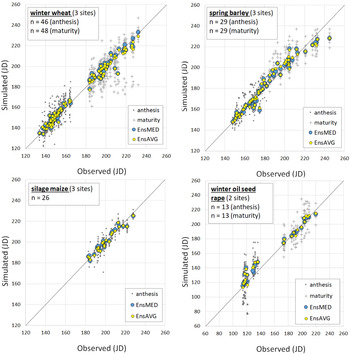
The simulations for winter wheat anthesis across all the sites showed (see Table 4 and Fig. 2) that CROPSYST and DAISY_1 simulated anthesis very well, with an IA of 0.96, followed by all other models whose results were satisfactory (IA varied from 0.84 to 0.95, except -FASSET with an IA of 0.37). Regarding the absolute error, CROPSYST and DAISY_1 achieved RMSEs equal to 2.9 days across all the sites, and the remaining models (except FASSET, which had an RMSE equal 12.6 days) achieved RMSEs ranging from 3.2 to 8.3 days. Fully comparable results with the best models for all sites together were achieved by EnsMED (IA = 0.97, MBE = 0.8 days, and RMSE = 2.9 days). EnsAVG showed a slightly lower accuracy (IA = 0.96, MBE = 1.2 days, and RMSE = 3.2 days).
Table 4. The evaluation according to the statistical parameters MBE (mean bias error), RMSE (root mean square error) and IA (index of agreement) for anthesis dates of winter wheat, spring barley, silage maize and winter oilseed rape

The evaluation involves individual experimental sites Lednice, Věrovany, Domanínek (abb. LED, VER, and DOM), respectively, and results from all the sites together. The medians (abb. EnsMED) and means (abb. EnsAVG) derived from all the model results were compared with observed data as well. Winter oilseed rape simulations within Věrovany were unavailable. When the RMSE of a model for all sites is higher than the mean RMSE plus 1.5 times the standard deviation for a certain crop, the name of a model is written in italics.

Fig. 2. Comparisons of observed and estimated anthesis (circles) and maturity (crosses) in days of the year (JD). The results based on individual model simulations are depicted in grey (or are apparent from Supplements 1–7), while the medians (EnsMED) and means (EnsAVG) from all the models for specific site-year combinations are in blue and yellow, respectively. Maturity for silage maize was not considered.
For spring barley anthesis, the best agreement was achieved by AQUACROP (all sites considered), with an IA of 0.96, MBE of 1.6 days and RMSE of 4.0 days. Models CROPSYST, DAISY_2, DSSAT_2, DSSAT_3, EPIC and MONICA achieved very similar IAs (0.95). Again, the FASSET model gave the least precise results for spring barley, but was more accurate than for winter wheat, with an IA equal to 0.77, an RMSE of 9.5 days, and simulated anthesis was systematically 7.6 days earlier (based on MBE and across all sites). EnsMED and EnsAVG provided results comparable to the best models for spring barley (IAs = 0.96, MBEs −0.6 and 0.0 days, respectively, RMSEs 4.0 and 3.7 days, respectively).
For silage maize anthesis, the AQUACROP and DAISY_1 models had the highest IA of 0.98 for all the sites. The remaining models (except FASSET) also had very satisfactory results, with IAs varying from 0.97 to 0.94 (for all the sites). The lowest value of IA (0.85) corresponded to the FASSET model. The systematic error MBEs varied from −3.0 to 1.6 days, and the absolute errors (RMSE) varied from 2.8 to 9.1 days based on individual models and considering all the sites together. EnsMED and EnsAVG had the highest indexes of agreement, 0.98 and 0.99, respectively, considering all the sites, with systematic errors of 0.1 and −0.2 days, respectively, and RMSEs of 3.0 and 2.7 days, respectively.
Although flowering was successfully estimated for the previous three crops (except for FASSET in the case of winter wheat), for winter oilseed rape, lower accuracy was generally achieved, either in terms of individual models or based on EnsMED and EnsAVG. For all the sites, the highest IAs were achieved by MONICA (0.91), AQUACROP (0.90) and FASSET (0.89). AGROTOOL had the lowest accuracy, with an IA equal to 0.38 and systematic and absolute errors of ~1 month. The general feature was a later estimate of the time of flowering (more pronouncedly in the cooler location of Domanínek). Only in the case of winter oilseed rape did EnsMED and EnsAVG produce worse results than the best individual models. Using EnsMED and EnsAVG, the indexes of the agreement were 0.76 and 0.73, respectively, the MBEs were 7.7 and 9.2 days, respectively, and the RMSEs were 9.8 and 11.5 days, respectively (considering all the sites).
Generally, the anthesis dates for winter wheat, spring barley and winter rape were overestimated (later than observed) in the case of the coolest station, Domanínek.
Maturity
In terms of winter wheat maturity, the highest IA (equal to 0.98) was achieved for model DAISY_1, with a low MBE at 1.1 days and an RMSE of 3.9 days (see Table 5). The IAs for the remaining models, except FASSET, which in this case also provided the least accurate results, varied from 0.86 to 0.96 (MBEs from −7.0 to 5.9 days and RMSEs from 4.6 to 10.8 days). Repeatedly, the FASSET model showed the poorest agreement (IA = 0.42, MBE = −16.5 days and RMSE = 24.2 days). EnsMED and EnsAVG had IAs of 0.96, MBEs in the range of −0.6 to −1.6 days and RMSEs from 4.8 to 5.0 days, respectively. Both EnsMED and EnsAVG were also able to produce reasonable values when obvious model outliers appeared (see Fig. 2, winter wheat).
Table 5. The evaluation of models according to the statistical parameters MBE (mean bias error), RMSE (root mean square error) and IA (index of agreement) for the maturity of winter wheat, spring barley and winter oilseed rape
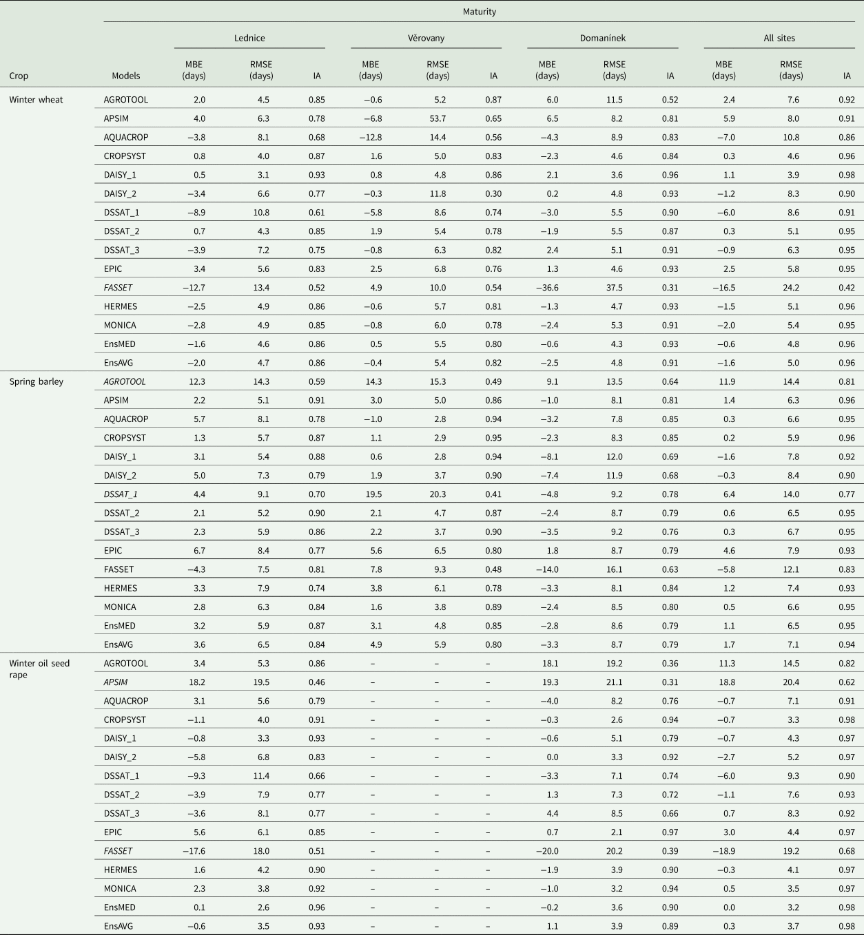
The evaluation involved individual experimental sites Lednice, Věrovany and Domanínek (abb. LED, VER and DOM, respectively) and the results from all the sites together. The medians (abb. EnsMED) and means (abb. EnsAVG) derived from all the model results were compared with observed data as well. Winter oilseed rape simulations for the Věrovany site were unavailable. When the RMSE of a model for all sites is higher than the mean RMSE plus 1.5 times the standard deviation for a certain crop, the name of a model is written in italics.
Similar results were achieved for the simulations of spring barley maturity but with more accurate results in the case of FASSET (against winter wheat). Regarding the IA, the APSIM and CROPSYST models achieved the highest values (0.96) for all the sites. AQUACROP along with DSSAT_2, DSSAT_3 and MONICA reached IAs equal to 0.95. The least accurate results were attained by DSSAT_1, with an IA of 0.77 connected with a systematically later prediction of anthesis (MBE = 6.4 days) and high absolute error (RMSE = 14.0 days). The high values of MBE (11.9 days) and RMSE (14.4 days) were also achieved by the AGROTOOL model. Using EnsMED and EnsAVG, the IAs were 0.95 and 0.94, the MBEs were 1.1 and 1.7 days, and the RMSEs were 6.5 and 7.1 days, respectively (considering all the sites); this indicates slightly lower accuracy, as in the case of anthesis. A majority of the models and, consequently, the ensemble tools had problems reproducing very late spring barley maturity dates in the case of Domanínek (see Fig. 2 and Supplement 6).
In contrast to anthesis, winter oilseed rape maturity was better estimated by the models. For CROPSYST, the IA was 0.98, and for DAISY_1, DAISY_2, EPIC, HERMES and MONICA, the IAs was equal to 0.97 considering all the sites together. The other models IA ranged from 0.62 to 0.93. For most of the models, the MBEs varied from −6.0 to 3.0 days, and the RMSEs from 3.3 to 9.3 days (considering all the sites). AGROTOOL, APSIM and FASSET presented systematic errors ranged from −18.9 to 18.8 days, and absolute errors ranged from 14.5 to 20.4 days. Using EnsMED and EnsAVG, the IAs of 0.98 for both methods were achieved with MBEs of 0.0 and 0.3 days and RMSEs from 3.2 to 3.7 days, respectively. The observed date of maturity for maize was unavailable because it was harvested for silage.
Yield
The yields were simulated with considerably lower accuracy (compared to phenology) by both the models and the ensemble methods, as is apparent from Fig. 3 and Table 6. For the winter wheat yield, the models reached IAs ranging from 0.24 to 0.60 considering all sites together, where the highest value was recorded for the AQUACROP model and the lowest IA by MONICA (0.24). The MBEs varied from −1274 kg/ha (AGROTOOL) to 1057 kg/ha (DAISY_2), whereas the lowest MBE was achieved by CROPSYST at a level of −4 kg/ha. The RMSEs varied from 1326 kg/ha (AQUACROP) to 2828 kg/ha (DAISY_2). Six out of all 13 models achieved greater or equal IAs with respect to EnsMED (IA = 0.48). The IA for EnsAVG was 0.46. Thus, from the perspective of MBE and RMSE, EnsMED and EnsAVG still performed reasonably and are comparable to the best models (MBEs of 88 and 141 kg/ha, RMSEs of 1365 and 1439 kg/ha for EnsMED and EnsAVG, respectively). Although the individual runs resulted in highly variable winter wheat yield outputs (~10 tons/ha based on the difference between the minimal and maximal values of all runs) compared to the observed variability (about 7 t/ha), using EnsMED and EnsAVG for the seasonal yield resulted in an even lower variability of ~3 t/ha. This feature is similar for all crops, as can be seen in Fig. 4, where a comparison of the observed yield variability with each model and its ensemble (both as EnsAVG and EnsMED) can be seen. This figure shows that the higher variability of simulated yields (when considering all runs together) is mainly due to the differences between individual models than to the variability within the outputs of the single models.

Fig. 3. Comparisons of observed and simulated yield (in kg/ha) within 13 crop growth models for winter wheat, spring barley, silage maize and winter oilseed rape. The results based on individual model simulations are depicted in grey (or are apparent from Supplements 8–11), while the medians (EnsMED) and means (EnsAVG) from all the models for specific site-year combinations are in blue and yellow, respectively.

Fig. 4. Boxplots for values of observed and estimated yields by the models and on the ensemble basis. The boxes delimit the medians and interquartile ranges (25–75 percentiles), and the whiskers link the high and low extreme values.
Table 6. Model evaluation according to the statistical parameters MBE (mean bias error), RMSE (root mean square error) and IA (index of agreement) for yields of winter wheat, spring barley, silage maize and winter oilseed rape

The evaluation involved the individual Lednice, Věrovany and Domanínek (abb. LED, VER and DOM, respectively) experimental sites and results from all the sites together. Median (abb. EnsMED) and mean (abb. EnsAVG) derived from all the model results were compared with observed data as well. When the RMSE of a model for all sites is higher than the mean RMSE plus 1.5 times the standard deviation for a certain crop, the name of a model is written in italics.
For spring barley yield, the models achieved better estimates than for winter wheat (Table 6); the AQUACROP model obtained the highest IA (0.87), with an MBE equal to −151 kg/ha and an RMSE equal to 807 kg/ha when all the sites are considered. The lowest IA was observed for the MONICA model, i.e. 0.32. For the other models, the IAs varied from 0.36 to 0.74 for all the sites. Three models (AQUACROP, EPIC, CROPSYST) achieved better results for annual yield estimates with respect to using EnsMED, which had an IA of 0.64. The IA for EnsAVG was 0.61. The ensemble MBEs were −148 and −190 kg/ha, the RMSEs ranged from 1105 to 1136 kg/ha.
For silage maize yield, large differences also existed among the models, as is apparent from Table 6. Specifically, the AQUACROP model provided the highest value of IA, which was equal to 0.93 if all the sites were considered together. The other models had IAs ranging from 0.32 (AGROTOOL) to 0.84 (CROPSYST), MBE varied from −6784 to 716 kg/ha, and the RMSEs varied from 1355 to 7674 kg/ha. Among the individual localities, the AQUACROP model simulated Domanínek very accurately (IA = 0.96; MBE = 216 kg/ha, and RMSE = 1325 kg/ha). On the other hand, almost all the models underestimated the observed highest yield (Fig. 3) from the most fertile station, Věrovany. Based on IA, two of the models were better than EnsMED, and seven of the models were better than EnsAVG. Based on the IA, the ensemble models were able to most accurately simulate (compared to all the tested crops) silage maize yield.
The winter oilseed rape yield results are shown in Table 6 and Figs 3 and 4. Across all the sites, the highest value of IA was recorded for the EPIC model (0.74). On the other hand, the DSSAT_3 model had the lowest overall value of IA (0.20). Among the individual sites, the Lednice experimental site, especially when using the EPIC model, achieved the highest value of IA (0.84). The MBE and RMSE for the EPIC model and Lednice were 40 and 731 kg/ha, respectively. Generally, MBE and RMSE, based on individual models, varied from −518 to 815 kg/ha and from 719 to 1466 kg/ha, respectively (all sites considered together). Although the variabilities among the models are clear, EnsMED and EnsAVG produced quite narrow and low variable estimates close to 4 t/ha on average (see Fig. 4 for winter oilseed rape). Based on IA, the lowest agreements between the simulated (both by individual models and ensemble products) and observed yield were achieved for winter oilseed rape. For winter wheat, spring barley and silage maize, EnsMED produced more accurate yield estimates than EnsAVG (based on MBE, RMSE and IA). For winter oilseed rape, a lower IA for EnsMED was achieved (against EnsAVG) but also with lower MBE and RMSE.
Table 7 depicts a general overview of the observed and simulated yield of the four crops, including the ranges of errors, indexes of agreement and best performing simulations/models (based on all the statistical parameters individually). Overall and considering RMSE and IA, AQUACROP performed best for winter wheat, spring barley and silage maize, whereas EPIC performed best for winter oilseed rape. Although these models performed well overall, individual models outperformed the obtained results for specific locations or different statistical metrics. For example, considering MBE, CROPSYST performed best overall for winter wheat, DSSAT1 performed best for spring barley and MONICA performed best for silage maize and winter oilseed rape.
Table 7. Observed and simulated ranges of yields for all the sites and seasons using mean and ± standard deviation and agreements between simulated and observed yields using MBE, RMSE and IA

The most precise models are indicated using abbreviations within brackets
Figure 5 depicts the arrangement of models in order of their accuracies (considering average order based on RMSE and IA) for phenology, yields and their combination. The most successful models are AQUACROP and EPIC, but the best predictions were based on ensemble products. Considering all parameters and crops, EnsMED achieved the best results according to this evaluation. This was true at each individual station (so regardless of the climatic conditions) as well as considering all stations together. The EnsAVG indicator was in the second place if all stations are considered together, and in the individual stations, it was twice in the second place (Lednice, Věrovany) and once on the fourth place (Domanínek). CROPSYST is fine overall but not for estimated winter oilseed rape yield, low leaf area and high harvest index (see Figs 6 and 7). The AGROTOOL model resulted in less accurate results in general, and FASSET experienced some difficulties when reproducing crop phenology. For some models (AQUACROP, CROPSYST, DSSAT_3) a different behaviour (lower order) was found in the case of winter oilseed rape yields compared to the remaining crops in the case of the achieved order of models (Fig. 5b).
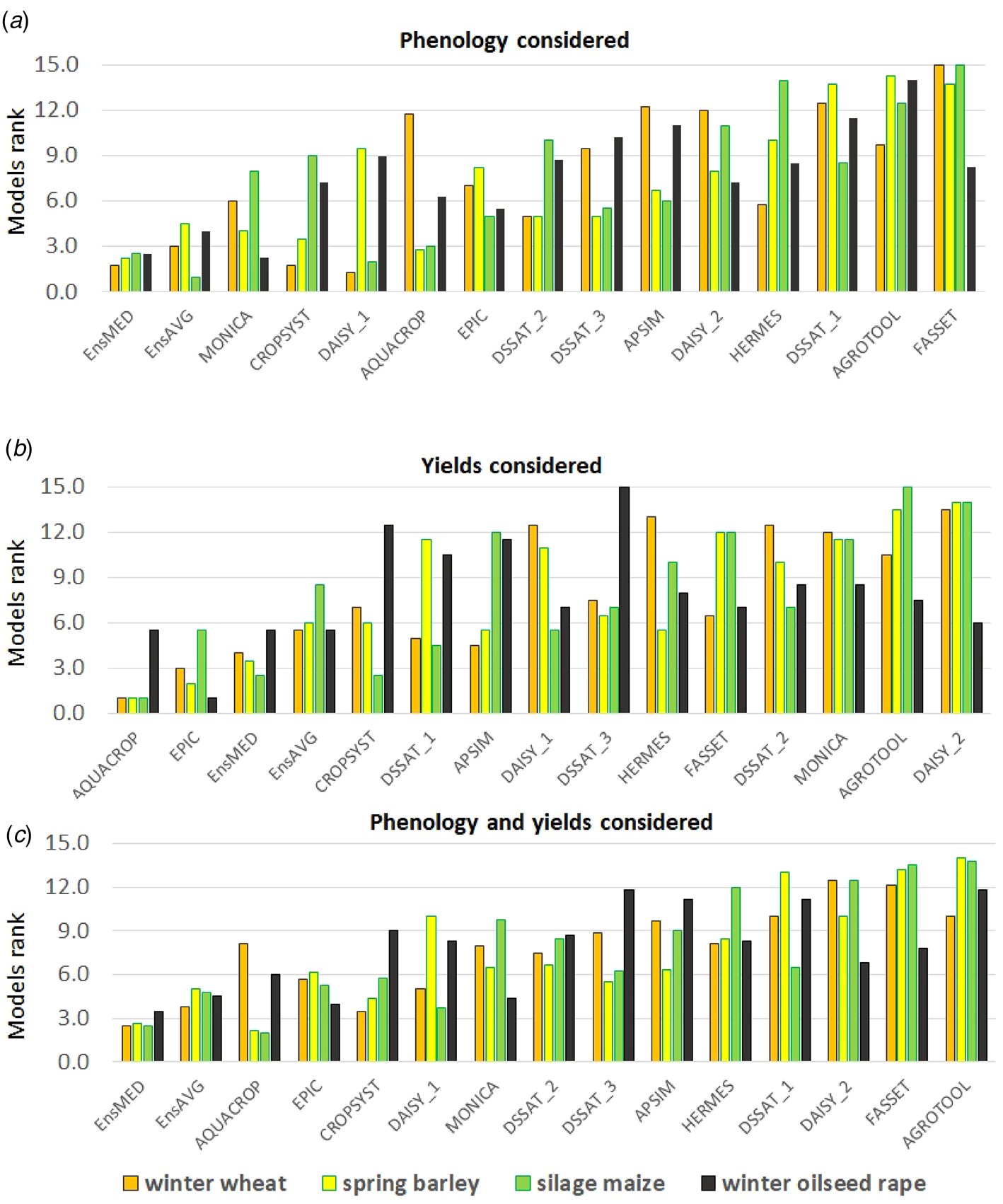
Fig. 5. Arrangement of the crop model tools based on RMSE and IA for phenology (a), yield (b) and combined for both phenology and yields (c) through the tested four crops and within the three experimental sites.

Fig. 6. Boxplots for maximum values of leaf area indexes during the season (LAImax) by the models. The comparisons include medians from single models, processed data from all the simulations, and averages and medians of the model ensemble for all the crops. The boxes delimit the interquartile ranges (25–75 percentiles), and the whiskers link the high and low extreme values.

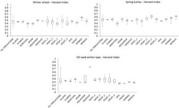
Fig. 7. Boxplots for values of harvest indexes within the employed models. The comparisons include medians from the single models, processed data from all the simulations, and the averages and medians of the model ensemble for all the crops. The boxes delimit the interquartile ranges (25–75 percentiles), and the whiskers link the high and low extreme values.
Although the study is not based on data from crop rotation experiments, the 112 seasons (sum through all crops) with observed yield bring the opportunity to evaluate the set of crops and models under uniform methodology. In the current study, IA was higher when simulating the development stages than when simulating yield. In the case of anthesis, the timing was simulated at similar levels of accuracy for winter wheat, spring barley and silage maize but less satisfactory for winter oilseed rape. On the other hand, IA for the maturity of winter oilseed rape was higher. In the cases of winter wheat and spring barley, the results were worse for maturity compared to anthesis. For most of the crops, no significant feature was identified between simulations, except at the Lednice station (warmer and drier), where the models' performances were better for the anthesis of winter oilseed rape when compared to those for Domanínek (colder and wetter).
Discussion
Crop yield prediction is at a less accurate level compared to phenology. One of the reasons is that the yield formation process is naturally more complex than phenology, as soil conditions and processes as well as biomass production and allocation, including root growth, which has large effects on water and nutrient availability, are estimated. One explanation for weaker model performances in simulating interannual and site variabilities could be related to the fact that crops within the experimental sites were not always grown on exactly the same plots over the years. Although the representative soil profiles for each trial site in the current study used estimated initial conditions as inputs to the crop growth models, slight deviations in the defined soil properties between years could affect the results. Moreover, spatial variations of soil conditions could exist within plots affecting the representation of soil model inputs. These factors can be one source of uncertainty, which may partly explain the spread of model outputs and correspondence with observed values. At the same time, however, it can be said, that the quality of the soil input data can be considered as completely appropriate to the concept of minimum calibration, also with respect that they are used by CISTA for description of field experiment conditions. Furthermore, although some models responded very sensitively to differences in site conditions, e.g. soil, water and nitrogen supply, others are less sensitive (Zhao et al., Reference Zhao, Hoffmann, Yeluripati, Specka, Nendel, Coucheney, Kuhnert, Tao, Constantin, Raynal, Teixeira, Grosz, Doro, Kiese, Eckersten, Haas, Cammarano, Kassie, Moriondo, Trombi, Bindi, Biernath, Heinlein, Klein, Priesack, Lewan, Kersebaum, Rötter, Roggero, Wallach, Asseng, Siebert, Gaiser and Ewert2016; Wallor et al., Reference Wallor, Kersebaum, Ventrella, Bindi, Cammarano, Coucheney, Gaiser, Garofalo, Giglio, Giola, Hoffmann, Iocola, Lana, Lewan, Maharjan, Moriondo, Mula, Nendel, Pohankova, Roggero, Trnka and Trombi2018). Another point is that yield extremes, especially at the lower end, are often caused by environmental conditions that most models have no available algorithm to represent their impact. For example, the influences of pests, diseases and other adverse conditions such as lodging, harvest losses and damage caused by rodents (e.g. Nendel et al., Reference Nendel, Wieland, Mirschel, Specka, Guddat and Kersebaum2013; Gobin, Reference Gobin2018) were not directly considered by the crop models. To understand some model overestimations, modellers need to have a good description or database of how observed yield decreases can be explained. No information or evidence was available in the study database on the actual occurrence of phenomena such as lodging, hail, pest and diseases, etc. which could cause some reduction in the observed yield.
Considering yield combined for all sites, the best models (e.g. AQUACROP, EPIC) produced higher IAs than EnsMED and EnsAVG. This is in agreement with Soltani and Sinclair (Reference Soltani and Sinclair2015), as simpler models tend to be more robust. The better results from some individual models (against the ensemble outputs) are not in line with the results of previous studies (e.g. Asseng et al., Reference Asseng, Ewert, Martre, Rötter, Lobell, Cammarano, Kimball, Ottman, Wall, White, Reynolds, Alderman, Prasad, Aggarwal, Anothai, Basso, Biernath, Challinor, De Sanctis, Doltra, Fereres, Garcia-Vila, Gayler, Hoogenboom, Hunt, Izaurralde, Jabloun, Jones, Kersebaum, Koehler, Müller, Naresh Kumar, Nendel, O’Leary, Olesen, Palosuo, Priesack, Eyshi Rezaei, Ruane, Semenov, Shcherbak, Stöckle, Stratonovitch, Streck, Supit, Tao, Thorburn, Waha, Wang, Wallach, Wolf, Zhao and Zhu2015), which concluded that EnsMED is more accurate than any individual member in simulating the response of crop (as determined from experiments and observations across a wide range of environments). In addition, Martre et al. (Reference Martre, Wallach, Asseng, Ewert, Jones, Rötter, Boote, Ruane, Thorburn, Cammarano, Hatfield, Rosenzweig, Aggarwal, Angulo, Basso, Bertuzzi, Biernath, Brisson, Challinor, Doltra, Gayler, Goldberg, Grant, Heng, Hooker, Hunt, Ingwersen, Izaurralde, Kersebaum, Müller, Kumar, Nendel, o'Leary, Olesen, Osborne, Palosuo, Priesack, Ripoche, Semenov, Shcherbak, Steduto, Stöckle, Stratonovitch, Streck, Supit, Tao, Travasso, Waha, White and Wolf2015) found both median and mean estimates to be better predictors than any individual model outcomes. However, collecting a high number of members within the ensemble still does assure that certain ensemble outcomes or their interpretation might not change if some members were added or removed from the ensemble (e.g. Rodriguez et al., Reference Rodríguez, Ruiz-ramos, Palosuo, Carter, Fronzek, Lorite, Ferrise, Pirttioja, Bindi, Baranowski, Buis, Cammarano, Chen, Dumont, Ewert, Gaiser, Hlavinka, Ho, Höhn, Jurecka, Kersebaum, Trnka, De Wit and Rötter2018).
Another point to consider is model accuracy across all the sites together or at each single site where other models may achieve better results. For instance, for winter wheat at Věrovany, EPIC can be ranked first (lowest RMSE and highest IA), whereas AQUACROP's IA is fourth lowest. Therefore, when it comes to selecting the best model(s) or ensemble composition (based on a set of models with the best performance) for specific conditions or range of conditions, the priority between accuracy and robustness (maintaining good performance in different environments) should be resolved. This can be supported by a good calibration and validation procedure, for which detailed and extensive databases are absolutely essential. Especially in the case of more complex models, this plays an important role, where detailed information is crucial for calibration. Based on the results of global large model ensemble studies, pre-selection of models would not be possible due to their complexity and it is not always true that higher complexity means higher accuracy. For example, a model such as Aquacrop may be preferred when information is limited (Confalonieri et al., Reference Confalonieri, Orlando, Paleari, Stella, Gilardelli, Movedi, Pagani, Cappelli, Vertemara, Alberti, Alberti, Atanassiu, Bonaiti, Cappelletti, Ceruti, Confalonieri, Corgatelli, Corti, Dell'Oro, Ghidoni, Lamarta, Maghini, Mambretti, Manchia, Massoni, Mutti, Pariani, Pasini, Pesenti, Pizzamiglio, Ravasio, Rea, Santorsola, Serafini, Slavazza and Acutis2016).
In addition to the models' characteristics, the variation in modellers' knowledge, experiences, parametrization and subjective approaches for study-specific conditions and target crops could be factors affecting accuracy, as the same models (DAISY_1 v. DAISY_2 and DSSAT_1 v. DSSAT_2 v. DSSAT_3) did not produce the same phenology or yield (Figs 4 and 5). The input data was the same, but the parameter settings differed for each model. Generally, for phenology, lower differences between the same models (except DAISY for winter oilseed rape anthesis) resulted with respect to yield. The differences between the same models are also evident within the maximum estimated values of leaf area index (Fig. 6), especially for DSSAT models. On the other hand, the harvest index results were more stable between the same models as well as through all the models (Fig. 7).
Generally, the highest variability in modelled annual yield was achieved considering individual models. For example, in our study, simulated winter wheat yield ranged from 2164 to 12 185 kg/ha, whereas the observed yield range was narrower, 2442 to 9297 kg/ha, across all the sites. A similar trend was achieved by Palosuo et al. (Reference Palosuo, Kersebaum, Angulo, Hlavinka, Moriondo, Olesen, Patil, Ruget, Rumbaur, Takac, Trnka, Bindi, Caldag, Ewert, Ferrise, Mirschel, Saylan, Siska and Rötter2011), in which the modelled winter wheat yield results ranged from 1800 to 12 000 kg/ha compared against a similar real yield range. Here, the same field experiments with Samanta variety in Lednice and Věrovany were included. The different feature of the mentioned study was that several of their models showed a larger yield range than the observed data. Palosuo et al. (Reference Palosuo, Kersebaum, Angulo, Hlavinka, Moriondo, Olesen, Patil, Ruget, Rumbaur, Takac, Trnka, Bindi, Caldag, Ewert, Ferrise, Mirschel, Saylan, Siska and Rötter2011) also listed a wide range of IA (0.40–0.74) and RMSE (1400–2300 kg/ha) for winter wheat and similarly Rötter et al. (Reference Rötter, Palosuo, Christian, Angulo, Bindi, Ewert, Ferrise, Hlavinka, Moriondo, Nendel and Olesen2012) for spring barley (RMSE from 1120 to 1940 kg/ha and IA from 0.31 to 0.63). However, the observed yield was not known to the modellers for the model's setting.
The feature about lower reported variability by EnsMED and EnsAVG is not valid for phenology (Fig. 2), perhaps as an effect of the higher accuracies of individual models in phenology simulations compared to yield, where the errors of individual models are equally reduced. Based on the IAs for winter wheat, spring barley and silage maize, EnsMED produced more accurate estimates than EnsAVG, whereas, in the case of winter oilseed rape, that was reversed. The better performance of EnsMEDs is in accordance with results from previous multimodel ensemble studies and is reflected within the impact and adaptation studies (Pirttioja et al., Reference Pirttioja, Carter, Fronzek, Bindi, Hoffmann, Palosuo, Ruiz-Ramos, Tao, Trnka, Acutis, Asseng, Baranowski, Basso, Bodin, Buis, Cammarano, Deligios, Destain, Dumont, Ewert, Ferrise, Francois, Gaiser, Hlavinka, Jacquemin, Kersebaum, Kollas, Krzyszczak, Lorite, Minet, Minguez, Montesino, Moriondo, Muller, Nendel, Öztürk, Perego, Rodríguez, Ruane, Ruget, Sanna, Semenov, Slawinski, Stratonovitch, Supit, Waha, Wang, Wu, Zhao and Rötter2015; Ruiz-Ramos et al., Reference Ruiz-ramos, Ferrise, Rodríguez, Lorite, Bindi, Carter, Fronzek, Palosuo, Pirttioja, Baranowski, Buis, Cammarano, Chen, Dumont, Ewert, Gaiser, Hlavinka, Hoffmann, Höhn, Jurecka, Kersebaum, Krzyszczak, Lana, Mechiche-alami, Minet, Montesino, Nendel, Porter, Ruget, Semenov, Steinmetz, Stratonovitch, Supit, Tao, Trnka, De Wit and Rötter2018). In the case of an ensemble based on verified and suitable models for target crops, EnsAVG likely provides higher informative value, but when there is uncertainty regarding some of the models, less experience and a smaller number of studies for a crop, EnsAVG is more prone to bias due to the higher impact of a model failure (Wallach et al., Reference Wallach, Martre, Liu, Asseng, Ewert, Thorburn, van Ittersum, Aggarwal, Ahmed, Basso, Biernath, Cammarano, Challinor, De Sanctis, Dumont, Rezaei, Fereres, Fitzgerald, Gao, Garcia-Vila, Gayler, Girousse, Hoogenboom, Horan, Izaurralde, Jones, Kassie, Kersebaum, Klein, Koehler, Maiorano, Minoli, Müller, Naresh Kumar, Nendel, O'Leary, Palosuo, Priesack, Ripoche, Rötter, Semenov, Stöckle, Stratonovitch, Streck, Supit, Tao, Wolf and Zhang2018).
Using the ensemble, better yield results (IA-based) were achieved for spring crops, and worse results were obtained for winter crops. This is in contrast with Rötter et al. (Reference Rötter, Palosuo, Christian, Angulo, Bindi, Ewert, Ferrise, Hlavinka, Moriondo, Nendel and Olesen2012) who compared models for spring barley (represented by cultivar Orbit from the Lednice and Věrovany experiments conducted between 1984 and 1998) and concluded, using RMSE and IA, that models performed slightly, but not significantly, better for winter wheat. For instance, the worst results were achieved for yield of winter oilseed rape. This could be explained by the influence of overwintering conditions and modelling of connected impacts (low-temperature stresses, presence and influence of snow cover). Moreover, modellers' experience when simulating winter oilseed rape is usually lower, and the amount of data for calibration as well as the number of studies are much smaller than for main staple crops, e.g. wheat and maize (see e.g. Kollas et al., Reference Kollas, Kersebaum, Nendel, Manevski, Müller, Palosuo, Armas-Herrera, Beaudoin, Bindi, Charfeddine, Conradt, Constantin, Eitzinger, Ewert, Ferrise, Gaiser, De Cortazar-Atauri, Giglio, Hlavinka, Hoffmann, Hoffmann, Launay, Manderscheid, Mary, Mirschel, Moriondo, Olesen, Öztürk, Pacholski, Ripoche-Wachter, Roggero, Roncossek, Rötter, Ruget, Sharif, Trnka, Ventrella, Waha, Wegehenkel, Weigel and Wu2015) as it is obvious from the different number of studies focused on modelling of individual field crops (e.g. Web of Science, Orlandini et al., Reference Orlandini, Nejedlik, Eitzinger, Alexandrov, Toulios, Calanca, Trnka and Olesen2008). The relatively poor performance of most models for oilseed rape yields indicates that the database for many models for parameterizing oilseed rape was not sufficient so far or important crop-specific responses, e.g. frost damage and recovery, were not sufficiently considered in some models. In principle, however, the experience of modellers can influence simulation accuracy for all the crops involved, when the calibration procedure could by burdened to some extent due to the user's subjectivity. The example could be the possibility to simulate similar phenological development with different combinations of cardinal temperatures and thermal sums or due to the large variability in the values available in the literature for the parameters involved (Confalonieri et al., Reference Confalonieri, Orlando, Paleari, Stella, Gilardelli, Movedi, Pagani, Cappelli, Vertemara, Alberti, Alberti, Atanassiu, Bonaiti, Cappelletti, Ceruti, Confalonieri, Corgatelli, Corti, Dell'Oro, Ghidoni, Lamarta, Maghini, Mambretti, Manchia, Massoni, Mutti, Pariani, Pasini, Pesenti, Pizzamiglio, Ravasio, Rea, Santorsola, Serafini, Slavazza and Acutis2016). In consequence, extending research to less modelled crops such as winter oilseed rape is strongly recommended (e.g. Rötter et al., Reference Rötter, Appiah, Fichtler, Kersebaum, Trnka and Ho2018). In the case of CROPSYST, the robustness of winter oilseed rape should be reconsidered due to the very high harvest index results from the current study (Fig. 7). On the other hand, errors within some models under such conditions are quite surprising, and their reparameterization or improvement should be considered. Especially in the case of winter crops, the relative RMSEs (normalized by the average observed yield) for a majority of the models exceeded 20%, which could be considered as a threshold for successful calibration (e.g. Ruiz-Ramos et al., Reference Ruiz-ramos, Ferrise, Rodríguez, Lorite, Bindi, Carter, Fronzek, Palosuo, Pirttioja, Baranowski, Buis, Cammarano, Chen, Dumont, Ewert, Gaiser, Hlavinka, Hoffmann, Höhn, Jurecka, Kersebaum, Krzyszczak, Lana, Mechiche-alami, Minet, Montesino, Nendel, Porter, Ruget, Semenov, Steinmetz, Stratonovitch, Supit, Tao, Trnka, De Wit and Rötter2018).
The ability of models to explain yield variability could be attributed to the differences within their characteristics (Table 2). Consequences could be evident also from individual growth outputs such as the simulated maximum values of leaf area index during the season (LAIMAX) (Fig. 6). Relevant differences in leaf area index were reported for various models for winter wheat in Palosuo et al. (Reference Palosuo, Kersebaum, Angulo, Hlavinka, Moriondo, Olesen, Patil, Ruget, Rumbaur, Takac, Trnka, Bindi, Caldag, Ewert, Ferrise, Mirschel, Saylan, Siska and Rötter2011) as well. On the other hand, the reported harvest indexes by models were at a stable level (except CROPSYST for winter oilseed rape) in the current study (Fig. 7).
In some cases, the individual models failed completely, even for variables with known target values, e.g. FASSET for winter crops maturity dates and AGROTOOL for silage maize yield. Failure is defined here if the RMSE of a model to a specific target variable is higher than the mean RMSE of all models plus 1.5 times of the standard deviation (as it is indicated within Tables 4−6). This is another argument for preferring EnsMED to EnsAVG (or use at least both of them) to avoid effects due to simulated outliers in multi-model ensembles (Wallach et al., Reference Wallach, Martre, Liu, Asseng, Ewert, Thorburn, van Ittersum, Aggarwal, Ahmed, Basso, Biernath, Cammarano, Challinor, De Sanctis, Dumont, Rezaei, Fereres, Fitzgerald, Gao, Garcia-Vila, Gayler, Girousse, Hoogenboom, Horan, Izaurralde, Jones, Kassie, Kersebaum, Klein, Koehler, Maiorano, Minoli, Müller, Naresh Kumar, Nendel, O'Leary, Palosuo, Priesack, Ripoche, Rötter, Semenov, Stöckle, Stratonovitch, Streck, Supit, Tao, Wolf and Zhang2018). Using EnsMED and EnsAVG for seasonal yield estimates results in lower variability than the observed values. This is somewhat problematic in terms of the desired capability of model ensembles to simulate extremely low yield under adverse conditions (e.g. future droughts and heat stress). Simultaneously simpler models could also bring important robustness, but it is necessary to balance such approaches by the parallel use of more complex models, which allows more processes to be analyzed. In some cases, the yields formation based on the harvest index approach brings problems (e.g. in the case of winter oilseed rape by CROPSYST), but a similar approach was also used within the most successful of included models EPIC and AQUACROP (see Table 2). Fronzek et al. (Reference Fronzek, Pirttioja, Carter, Bindi, Ho, Palosuo, Ruiz-ramos, Tao, Trnka, Acutis, Asseng, Baranowski, Basso, Bodin, Buis, Cammarano, Deligios, Destain, Dumont, Ewert, Ferrise, François, Gaiser, Hlavinka, Jacquemin, Christian, Kollas, Krzyszczak, Lorite, Minet, Minguez, Montesino, Moriondo, Müller, Nendel, Öztürk, Perego, Rodríguez, Ruane, Ruget, Sanna, Semenov, Slawinski, Stratonovitch, Supit, Waha, Wang, Wu, Zhao and Rötter2018) provided insight into differences within wheat models behaviour and concluded about the closer correspondence of sensitivity to temperature and precipitation change in models using partitioning schemes for yield formation than in those using a harvest index approach.
Conclusions
The responses of the single models and the multi-model ensemble were not found to be consistent through all the tested crops, primarily because although there are countless calibration studies for winter wheat, spring barley and silage maize, a smaller number of studies have focused on winter oilseed rape, and modellers have less experience with modelling this crop. Hence, further calibration works and connected research are recommended for crops, that are less common for crop modellers. Also, such crops are necessary for successful simulations of crop rotations and more complex soil–atmosphere–crop–farmer interaction assessments.
It can be concluded that even in cases when yields are known, there are significant differences in results between individual models. In general, spring crop yield was simulated more satisfactorily than winter crops. The poorest results were obtained for winter oilseed rape.
For correct ensemble crop rotation simulations, only models with reasonable accuracy (i.e. without failures) across all included crops and investigated variables within the target environment (which is not automatic) should be selected and based on robust calibration/verification studies. Modelling of anthesis and maturity was generally best simulated by the ensemble compared to the individual model results, whereas EnsMED is better than EnsAVG. The yield was better estimated by the best models than by the tested ensemble, which nevertheless provided robust results. Considering RMSE and IA, and all the sites together, AQUACROP resulted in the best model for simulating the yield of winter wheat, spring barley, and silage maize, and EPIC resulted in the best model for winter oilseed rape. Regarding the MBE metric, CROPSYST was best for winter wheat, DSSAT1 was best for spring barley, and MONICA was best for silage maize and winter oilseed rape. Taking into account phenology and yields together, EnsMED was identified as the most universal predictor (compared to EnsAVG and individual crop models). This was also proved within the individual stations, so across the tested climatic conditions. This is despite ensemble composition and the inclusion of less accurate models. Some degree of simulations uncertainty could be connected to the user´s subjectivity within the calibration process. Also, in this case, the ensemble approach (including ensembles of the same models) can help increase the accuracy and robustness of estimates and with quantification of uncertainty. Achieved results together with the characteristic lower variability of ensemble outputs against the observed values can be used for planning and interpretation of studies focused on the impacts of changed agrometeorological conditions on individual crops as well as crop rotations.
Supplementary material
The supplementary material for this article can be found at https://doi.org/10.1017/S0021859621000216
Financial Support
This work is part of the research supported by the projects:
− SustES – Adaptation strategies for sustainable ecosystem services and food security under adverse environmental conditions (CZ.02.1.01/0.0/0.0/16_019/0000797);
− IGA AF MENDELU No. TP 7/2015 with the support of the Specific University Research Grant, provided by the Ministry of Education, Youth and Sports of the Czech Republic;
− the I4S Project within the BMBF BonaRes Program (031B0513I);
− RPR was supported by the German Federal Ministry of Education and Research (BMBF) via the BARISTA project (031B0811A) and via SALLnet (01LL1304A);
− Scientific support of climate change adaptation in agriculture and mitigation of soil degradation (ITMS2014+ 313011W580) supported by the Integrated Infrastructure Operational Programme funded by the ERDF’;
− MRR and AR were supported by Spanish National Institute for Agricultural and Food Research and Technology and
− Agencia Estatal de Investigación;
− Grant MACSUR02 – APCIN2016-0005-00-00;
− RF, CD, DV, LG and MM acknowledge financial support from MACSUR-2 knowledge hub funded for the Italian partnership by the Ministry of Agricultural, Food and Forestry Policies (D.M. 24064/7303/15 of 16/Nov/2015);
− SUSTAg project (INIA, 652915 ERA-NET co-funded by FACCE-SURPLUS);
− the Comunidad de Madrid (Spain) and structural funds 2014-2020 (ERDF and ESF);
− project AGRISOST-CM S2018/BAA-4330;
− Spanish MINECO AgroScena-UP (PID2019-107972RB-I00).
Conflict of interest
None.
Ethical standards
Not applicable.


 Open access