


1. Introduction
Coherent structures including horseshoe vortices and very-large-scale structures in the near and intermediate fields of an axisymmetric jet issuing from a contracting nozzle are the subject of this study. The near field, which appears only for jets exiting from a contracting nozzle, is defined by its potential core, and is usually within  $z/d=0-7$ (z is the streamwise direction and d is the jet nozzle diameter). The far field, located from approximately
  $z/d \geq 70$, is the self-similar region of the jet. The intermediate field is the streamwise region between the near and far fields and becomes fully turbulent from approximately
  $z/d=10$ (Ball, Fellouah & Pollard Reference Ball, Fellouah and Pollard2012). It is noted that the onset of the self-similar region for various free shear flows such as axisymmetric turbulent wakes (Dairay, Obligado & Vassilicos Reference Dairay, Obligado and Vassilicos2015) and turbulent planar jets (Cafiero & Vassilicos Reference Cafiero and Vassilicos2019) has been reconsidered recently.
A coherent structure is defined as a connected, large-scale turbulent fluid mass, with a phase-correlated vorticity over its spatial extent (Hussain Reference Hussain1983), and survives long enough to be traceable in a flow visualization movie and/or contribute significantly to time-averaged statistics of the turbulent flow (Adrian Reference Adrian2007); i.e. it is coherent in time and space. Such structures are known to contribute significantly to noise generation (Crow & Champagne Reference Crow and Champagne1971; Mankbadi & Liu Reference Mankbadi and Liu1984; Cavalieri et al. Reference Cavalieri, Rodríguez, Jordan, Colonius and Gervais2013; Fu et al. Reference Fu, Agarwal, Cavalieri, Jordan and Brès2017), mixing and entrainment (Winant & Browand Reference Winant and Browand1974; Philip & Marusic Reference Philip and Marusic2012) and drag (Orlandi & Jiménez Reference Orlandi and Jiménez1994; Schoppa & Hussain Reference Schoppa and Hussain1998; Abbassi et al. Reference Abbassi, Baars, Hutchins and Marusic2017). Therefore, a thorough understanding of their underlying physics can facilitate modelling and prediction of turbulent flows by breaking down the complex, multiscaled, seemingly random fields of turbulent motion into simpler orderly structures. Moreover, coherent structures and their interactions could be artificially magnified or suppressed through excitation or interruption imposed on the flow with the purpose of enhancing heat transfer, mixing and entrainment as well as drag reduction.
The existence of horseshoe/hairpin vortices, arch-like vortex tubes with one or both of their legs attached to the wall and their head parallel to the wall, in wall-bounded turbulent flows has long been acknowledged dating back at least to Theodorsen (Reference Theodorsen1952), who proposed the existence of such vortices as a dominant structure in turbulent boundary layers. Since then, hairpin vortices have been studied intensively in wall-bounded turbulence (see e.g. Falco Reference Falco1977; Head & Bandyopadhyay Reference Head and Bandyopadhyay1981; Ganapathisubramani et al. Reference Ganapathisubramani, Hutchins, Hambleton, Longmire and Marusic2005; Dennis & Nickels Reference Dennis and Nickels2011; Eitel-Amor et al. Reference Eitel-Amor, Örlü, Schlatter and Flores2015). These structures have also been used to model the turbulent boundary layer and predict various statistics in it successfully (see Marusic & Monty (Reference Marusic and Monty2019), and references therein). Hairpin vortices are the dominant structures in the logarithmic layer, and are understood to be responsible for the production of Reynolds shear stresses and turbulence kinetic energy through inducing ejections of low-speed fluid outward from the wall and sweeps of high-speed fluid inward toward the wall (Robinson Reference Robinson1991). Several experimental and numerical studies suggest that the hairpin vortices tend to spatially align in the streamwise direction, forming correlated packets or trains of vortices called hairpin packets (e.g. Adrian, Meinhart & Tomkins Reference Adrian, Meinhart and Tomkins2000; Marusic Reference Marusic2001; Ganapathisubramani, Longmire & Marusic Reference Ganapathisubramani, Longmire and Marusic2003). Moreover, these hairpin packets concatenate and form very long meandering regions of momentum deficit surrounded by high-speed fluid called superstructures or very large-scale motions (Hutchins & Marusic Reference Hutchins and Marusic2007; Lee, Sung & Adrian Reference Lee, Sung and Adrian2019; Eich et al. Reference Eich, de Silva, Marusic and Kähler2020). The contribution of superstructures to the streamwise turbulence kinetic energy increases with Reynolds number.
While horseshoe/hairpin vortices have been the subject of extensive research in wall-bounded turbulent flows and their significance has been manifested over several decades, they have received significantly less attention in the context of free shear flows. Based on the correlation measurements of three velocity components in turbulent free shear flows, Townsend (Reference Townsend1976) postulated that the free shear flow dynamics is dominated by double-roller eddy structures that are inclined to the axial direction. Following Townsend's hypothesis, Nickels & Perry (Reference Nickels and Perry1996) modelled the turbulent round jet using double-roller eddies with a characteristic radial length that is proportional to the characteristic radius of the jet and a limited azimuthal extent; a number of these structures are randomly distributed in different azimuthal and axial positions with equal probability to form the flow. They observed fairly good agreement between the Reynolds stresses and energy spectra calculated from this model compared with those from experiments.
Suto et al. (Reference Suto, Matsubara, Kobayashi, Watanabe and Matsudaira2004) used direct numerical simulations and experiments to study coherent structures in the turbulent round jet at a relatively low jet Reynolds number of  $Re_d=U_j d/\nu =1200$. Here,
  $U_j$,
  $d$ and
  $\nu$ are the jet exit mean velocity, the nozzle diameter and the kinematic viscosity of the fluid, respectively. Consistent with two-point correlations, they proposed a conceptual model of a horseshoe-like eddy in the jet. Their analyses revealed that the eddies stand with their legs inclined downstream at an inclination angle of
  $45^{\circ }$. These eddies were geometrically similar to those reported in wall-bounded flows. Matsuda & Sakakibara (Reference Matsuda and Sakakibara2005) used time-resolved stereo particle image velocimetry (PIV) measurements together with the frozen turbulence eddy hypothesis to form three-dimensional flow fields of the jet up to
  $Re_d = 5000$. They used isosurfaces of the swirling strength and revealed a group of horseshoe-like vortices around the rim of the shear region of the jet in the pseudo-instantaneous flow fields. Further, they used linear stochastic estimation to conditionally average these structures and found ring-shaped structures at the radial location
  $r=r_{0.5}$ and horseshoe-like structures at
  $r=1.5r_{0.5}$; here,
  $r_{0.5}$ is the jet half-radius. Recently, Samie, Lavoie & Pollard (Reference Samie, Lavoie and Pollard2020) applied a spectral correlation analysis to two-point measurement datasets with radial separations between the sensors in the jet, and showed that the eddy structures embedded in the turbulent jet are hierarchical rather than single sized.
Hairpin/horseshoe vortices have been documented in other unbounded shear flows as well. Vanderwel & Tavoularis (Reference Vanderwel and Tavoularis2011) reported both upright and inverted vortices in uniformly sheared turbulent flow. They observed that the dominant coherent structures of fully developed uniformly sheared flow are very different from the structures present in the flow exiting the shear-generating apparatus, which suggested that these hairpin-like structures are insensitive to initial conditions. Recently, Kirchner, Elliott & Dutton (Reference Kirchner, Elliott and Dutton2020) studied the near-wake flow structure behind a blunt-based cylinder aligned with a Mach 2.49 free stream using tomographic PIV, and observed upright and inverted hairpin structures throughout this flow. Using linear stochastic estimation, they conditionally averaged these structures and provided statistical evidence of their existence in various subregions of the flow.
Despite the lack of sufficient knowledge about horseshoe/hairpin vortices in round jet flow, coherent structures in the near field and far field of the jet have been investigated intensively in the past five decades or so. The vortex ring, which is formed as a result of large radial shear and Kelvin–Helmholtz instability in the near field of the axisymmetric jet, is known as the dominant coherent structure in this region, and has been investigated by many researchers (Crow & Champagne Reference Crow and Champagne1971; Browand & Laufer Reference Browand and Laufer1975; Yule Reference Yule1978; Liepmann & Gharib Reference Liepmann and Gharib1992, among others). Moving downstream, the vortex ring breaks into smaller structures due to the growth of azimuthal instabilities. Using two-dimensional laser-induced fluorescence images acquired at the round jet transverse planes at various streamwise locations, Liepmann & Gharib (Reference Liepmann and Gharib1992) showed that, as the jet progresses into the turbulent region, azimuthal instabilities break the vortex ring and produce axial vortex pairs in what is referred to as the braid region. Lacking a three-dimensional vision of this phenomenon, they concluded that streamwise vortices play a central role in the entrainment rate and in the dynamics of the jet. Jung, Gamard & George (Reference Jung, Gamard and George2004) used 138 hot-wires to acquire streamwise velocity fields at several cross-stream planes in the near field of the round jet. Applying proper orthogonal decomposition (POD) to the data at two diameters downstream of the jet nozzle, they observed structures that were similar to those reported by Liepmann & Gharib (Reference Liepmann and Gharib1992). More recently, the significance of streamwise vortices in the jet dynamics has been revisited by Davoust, Jacquin & Leclaire (Reference Davoust, Jacquin and Leclaire2012) and Nogueira et al. (Reference Nogueira, Cavalieri, Jordan and Jaunet2019) by applying POD and spectral proper orthogonal decomposition to two-dimensional PIV data acquired on cross-stream planes in the jet near field. Nogueira et al. (Reference Nogueira, Cavalieri, Jordan and Jaunet2019) observed that, similar to wall-bounded flows, large-scale streaky structures are present in the turbulent jet near field.
The intermediate and far fields of a turbulent round jet are dominated by axisymmetric, and single and double helix very-large-scale coherent structures (see e.g. Dimotakis, Miake-Lye & Papantoniou Reference Dimotakis, Miake-Lye and Papantoniou1983; Tso & Hussain Reference Tso and Hussain1989; Yoda, Hesselink & Mungal Reference Yoda, Hesselink and Mungal1994). Recently, Mullyadzhanov et al. (Reference Mullyadzhanov, Sandberg, Abdurakipov, George and Hanjalić2018) analysed results from direct numerical simulation (DNS) of a turbulent round jet issuing from a fully developed pipe, and showed that a propagating helical wave represents the optimal eigenfunction for the flow, and the first two mirror-symmetric modes, containing nearly  $5\,\%$ of the total turbulence kinetic energy, capture all significant very-large-scale features. Samie, Lavoie & Pollard (Reference Samie, Lavoie and Pollard2021) applied a spectral correlation analysis to two-point velocity datasets obtained in the turbulent region of the round jet with radial and azimuthal separations between the sensors. Using a data-driven spectral filter, they decomposed the streamwise velocity into an eddy structure component and a very-large-scale motion (VLSM) one. They used these filtered velocities to construct the eddy structure component and VLSM component of correlation maps, thereby concluding that helical structures were significant features of the jet intermediate field. Their conclusion was drawn based on two-dimensional axial–radial and axial–azimuthal data. Samie et al. (Reference Samie, Lavoie and Pollard2021) also postulated that the VLSMs are formed as a result of the concatenation of large-scale horseshoe vortices in a preferred order in the jet intermediate field.
Works of Nickels & Perry (Reference Nickels and Perry1996) and Nickels & Marusic (Reference Nickels and Marusic2001) highlight the contribution of horseshoe vortices to the Reynolds stresses, and Philip & Marusic (Reference Philip and Marusic2012) demonstrated the role of these coherent structures in the entrainment in turbulent jets. Despite the significance of horseshoe vortices in the dynamics of turbulent round jets, several questions about them remain unanswered or vaguely answered: (i) Is there any link between the horseshoe vortices and the large-scale streaky structures and streamwise vortices in the jet near field? (ii) Is there any link between the horseshoe vortices and the VLSMs in the jet far field? (iii) How do horseshoe vortices evolve with increasing distance from the jet origin? (iv) Are all horseshoe vortices in the jet upright (similar to the turbulent boundary layer), or are inverted horseshoe vortices also present in the jet (similar to the wake and uniformly sheared turbulent flows)? In this paper, these questions are addressed using a DNS jet dataset from Shin, Sandberg & Richardson (Reference Shin, Sandberg and Richardson2017) conducted at  $Re_d=7300$. To this end, three-dimensional coherent structures are visualized. Further, conditionally averaged three-dimensional horseshoe-like and very-large-scale coherent structures in the near and intermediate fields of the turbulent round jet are educed, and evolution of these structures and their interactions are inspected.
2. Numerical details
The simulations were conducted using the High Performance Solver for Aeroacoustic Research (HiPSTAR) compressible DNS code (Sandberg Reference Sandberg2013). The flow domain has a cylindrical configuration with a structured grid. The grid is stretched in the streamwise direction. A fifth-order finite differencing scheme is used for the axial and radial directions, along with a spectral decomposition in the azimuthal direction. The simulated fluid is treated as an ideal, incompressible gas, with the same density and temperature as the ambient fluid. The Reynolds number calculated based on the jet inlet diameter is 7300 and the initial Mach number is 0.304, based on the volumetric flow rate. The mean density and fluctuations around the mean remain smaller than  $0.6\,\%$ and
  $0.01\,\%$, respectively, of inlet density.
The mean exit velocity follows a top-hat profile up to a fixed radius, with half-cosine functions smoothly decreasing the velocity to 0 near the inlet walls. No-slip boundary conditions are imposed along the inlet walls. The mean velocity has a superimposed artificial turbulent profile with a turbulence intensity of  $1.68\,\%$, which is generated based on the method of Kempf, Wysocki & Pettit (Reference Kempf, Wysocki and Pettit2012). The statistically steady-state jet is established after 540 jet characteristic times
  $\tau$, with
  $\tau =d/U_j$, where
  $d$ is the nozzle diameter and
  $U_j$ is the jet exit velocity. The statistics and conditioned structures were obtained by temporal and spatial averaging 1585 independent flow fields; the spatial averaging is performed along the azimuthal direction due to statistical stationarity and azimuthal homogeneity of the round jet flow. A more detailed description of the code and numerical set-up can be found in Shin et al. (Reference Shin, Sandberg and Richardson2017).
3. Results and discussion
3.1. Quadrant analysis and azimuthal vorticity distribution
Horseshoe vortices are closely related to the Reynolds shear stress in wall-bounded turbulence. In fact, one of the main criteria to detect horseshoe vortices involves determining the mean turbulent flow field about a point where the flow makes a strong contribution to the mean Reynolds shear stress (Adrian Reference Adrian2007). Therefore, it seems reasonable to inspect the Reynolds shear stress,  $\overline {u_r u_z}$, in the turbulent jet. Here
  $u_r(=U_r-\overline {U_r})$ and
  $u_z(=U_z-\overline {U_z})$ denote the radial and streamwise fluctuating velocity components, respectively, and the overline indicates ensemble-averaged quantities. The contour map of Reynolds shear stress normalized by the centreline velocity,
  $\overline {u_r u_z}/U_{cl}^2$, against the normalized radial distance from the jet centreline,
  $r/d$, and the normalized axial distance from the jet nozzle,
  $z/d$, is displayed in figure 1. The locus of the maxima of the Reynolds shear stress is marked by the solid line, while the dashed lines correspond to the normalized shear stress level
  $\overline {u_r u_z}/U_{cl}^2=0.002$. The latter can be regarded as the indicator of the boundary between the shear and potential regions; the potential core is visible in the axial range
  $z/d=0-5$. Note that the criterion used to indicate the boundary between the shear and potential regions is not critical in our analysis, and any other indicator such as turbulence kinetic energy level or vorticity magnitude could be used instead. Nowhere in the jet field is the Reynolds shear stress negative, implying that, more often than not,
  $u_r$ and
  $u_z$ are of similar signs; that is,
  $u_r$ and
  $u_z$ are positively correlated in the turbulent jet. A quadrant analysis (Wallace, Eckelmann & Brodkey Reference Wallace, Eckelmann and Brodkey1972), which sorts the
  $u_r$ and
  $u_z$ fluctuations based on their sign, and presents their probability on a
  $u_r$–
 $u_z$ plane, can shed light on the contribution of various turbulent events to the Reynolds shear stress in the round jet.

Figure 1. The normalized Reynolds shear stress,  $\overline {u_r u_z}/U_{cl}^2$, as a function of
  $z/d$ and
  $r/d$. The solid line marks the locus of maxima of
  $\overline {u_r u_z}/U_{cl}^2$ while the dotted lines indicate the contour level
  $\overline {u_r u_z}/U_{cl}^2=0.002$.
In the quadrant analysis, the  $u_r$–
 $u_z$ plane is divided into 4 quadrants:
  $Q1$ where
  $u_r>0$ and
  $u_z>0$,
  $Q2$ where
  $u_r>0$ and
  $u_z<0$,
  $Q3$ where
  $u_r<0$ and
  $u_z<0$ and
  $Q4$ where
  ${u_r<0}$ and
  $u_z>0$. Here, a modified version of the quadrant analysis will be presented, which provides a better spatial understanding of these turbulent events (Kirchner et al. Reference Kirchner, Elliott and Dutton2020). To ensure that only the strong events associated with the large-scale horseshoe vortices are included in the analysis, first a three-dimensional (3-D) elliptic high-pass filter with the cutoff wavelengths
  $(\lambda _{r_c}, \lambda _{s_c}, \lambda _{z_c})=d\times (0.1,0.05,0.05)$ is applied to the flow fields. This filter attenuates fluid structures with wavelengths smaller than the cutoff wavelengths in the radial, azimuthal and axial directions. Then, a threshold,
  $H_Q=0.0004$, is chosen such that only the events that satisfy
  $| u_r u_z |/U_{cl}^2>H_Q$ are sorted into
  $Q1$–
$Q1$– $Q4$ bins. This is the concept of the ‘hyperbolic hole’ first introduced by Willmarth & Lu (Reference Willmarth and Lu1972). The sensitivity of the quadrant analysis to the threshold was tested by comparing
  $Q1/Q3-1$ contours for
  $H_Q=0.0001$, 0.0004 and 0.0016 and no difference was observed. Given that
  $\overline {u_r u_z}>0$ everywhere,
  $Q1$ and
  $Q3$ events are dominant in the jet; therefore, our focus will be on
  $Q1$ and
  $Q3$ events. These are displayed in figure 2(a–d) where contribution of
  $Q1$ and
  $Q3$ events to the jet turbulence against
  $r/d$ and
  $z/d$ in the near and intermediate fields are plotted as contour maps. Here, the solid and dashed lines are the same as those in figure 1. The
  $Q1$ and
  $Q3$ events outside the shear region are not taken into account as they do not contribute to the horseshoe vortex structures. It is evident that each of
  $Q1$ and
  $Q3$ events constitute between
  $30\,\%$ and
  $45\,\%$ of the total turbulent events. Furthermore,
  $Q3$ events dominate the outer edge of the shear region. For a better comparison of
  $Q1$ and
  $Q3$ events, contour maps of
  $Q1/Q3-1$ are plotted in figure 2(e,f), which illustrate that
  $Q3$ events are considerably more frequent than
  $Q1$ events in the outer part of the shear region in the jet near field, while their dominance is less noticeable in the outer part of the shear region in the intermediate field. On the other hand,
  $Q1$ events exhibit a clear dominance near the potential core in the jet near field. Contributions of
  $Q1$ and
  $Q3$ events appear to be virtually equal below the locus of the maxima of the Reynolds shear stress (solid line in figure 2f) in the jet intermediate field. It is stressed that the dominance of either
  $Q1$ or
  $Q3$ events in the near field is more conspicuous than that of
  $Q3$ events in the intermediate field. As it will be shown, this difference between the near and intermediate fields affects the conditionally averaged horseshoe vortices in these domains.

Figure 2. Percentage contribution of (a,b)  $Q1$ and (c,d)
  $Q3$ events to
  $\overline {u_r u_z}$. (e,f) Comparison of contributions of
  $Q1$ and
  $Q3$ events in the form of
  $Q1/Q3-1$. Panels (a), (c) and (e) are associated with the near field (
 $z/d=0-5$), while panels (b), (d) and (f) correspond to the intermediate field (
 $z/d=15-25$). The solid and dotted lines are same as those in figure 1. The open circle and square symbols in panel (e) indicate the location of conditional vortices displayed in figures 7 and 8, respectively. The open triangle and the filled star symbols in panel (f) indicate the location of conditional vortices illustrated in figures 9 and 12, respectively.
Another parameter that is closely associated with the horseshoe vortices in turbulent flows is the spanwise vorticity in wall-bounded flows, which is equivalent to the azimuthal vorticity ( $\omega _\theta$) in the axisymmetric jet. Elsinga et al. (Reference Elsinga, Adrian, Van Oudheusden and Scarano2010) and Dennis & Nickels (Reference Dennis and Nickels2011) selected the signed spanwise swirl (
 $\lambda _{ci,span} \cdot \mathrm {sign}(\omega _{span})$) as their conditional averaging event in wall-bounded turbulence. The spanwise swirl (
 $\lambda _{ci,span}$) is the characteristic swirl of a horseshoe vortex head; while it has no sign on its own, it can be signed using the spanwise vorticity via
  $\mathrm {sign}(\omega _{span})$. Similarly, Kirchner et al. (Reference Kirchner, Elliott and Dutton2020) adopted the negative component of the signed azimuthal swirl as the signature event for conditional averaging of the hairpin structures in the supersonic wake flow. The signed azimuthal swirl is closely related to the azimuthal vorticity (Kirchner et al. Reference Kirchner, Elliott and Dutton2020); therefore, it is crucial to determine whether positive azimuthal vorticity (
 $\omega _{\theta,p}$) or negative azimuthal vorticity (
 $\omega _{\theta,n}$) events prevail in different regions of the jet flow. Since only the
  $\omega _\theta$ events that correspond to the large-scale horseshoe vortices are of interest, a threshold
  $H_{\omega _\theta }=0.05$ is adopted such that
  $\omega _{\theta,p}/\omega _{\theta _{max}}>H_{\omega _\theta }$ and
  $\omega _{\theta,n}/\omega _{\theta _{max}}<-H_{\omega _\theta }$ need to be satisfied. Here,
  $\omega _{\theta _{max}}$ is the maximum of
  ${\omega _\theta }$ in the flow field. Figure 3 presents contour maps of
  $(\omega _{\theta,p}-\omega _{\theta,n})/\omega _{\theta,pmax}$ in which
  $\omega _{\theta,pmax}$ is the maximum of
  $\omega _{\theta,p}$. Similar to figure 2, the dashed lines indicate the shear region borders. In the near field,
  $\omega _{\theta,p}$ events are more frequent in the shear region close to the borders with the potential core and potential outer layer, while
  $\omega _{\theta,n}$ events prevail in the core of the shear region. In the intermediate field,
  $\omega _{\theta,p}$ events are predominant closer to the edge of the shear region, while
  $\omega _{\theta,n}$ events predominate in the region closer to the jet centreline. It is noted that adopting other values for
  $H_{\omega _\theta }$ in the range 0.05–0.1 does not affect conclusions drawn.

Figure 3. Comparison of the positive azimuthal vorticity,  $\omega _{\theta,p}$ and negative azimuthal vorticity,
  $\omega _{\theta,n}$, contribution to the total
  $\omega _\theta$ events presented as
  $(\omega _{\theta,p}-\omega _{\theta,n})/\omega _{\theta,pmax}$. (a) Near field. (b) Intermediate field. The lines and symbols are same as those in figure 2.
3.2. Horseshoe vortices
Horseshoe vortices and their association with ejection ( $Q2$) and sweep (
 $Q4$) events have been well studied in wall-bounded flows. It was shown in § 3.1 that
  $Q1$ and
  $Q3$ events dominate the turbulent fluctuations in the round jet. Here, we present sample instantaneous flow visualizations to demonstrate the correspondence between vortical structures and
  $Q1$ and
  $Q3$ events, and also the rationale behind the conditional averaging procedure used for the statistical analysis of vortical structures later. The swirling strength,
  $\lambda _{ci}$, will be used to visualize the vortical structures in the present study. The swirling strength criterion, introduced by Zhou et al. (Reference Zhou, Adrian, Balachandar and Kendall1999), uses the imaginary part of the complex eigenvalue of the velocity gradient tensor to identify vortical structures in the flow. Examples of typical 3-D instantaneous vortical structures (grey isosurfaces) in the jet near field, visualized by isosurfaces of
  $\lambda _{ci}$, are displayed in figure 4(a) and 4(c). Overlaid on the
  $\lambda _{ci}$ isosurfaces are the
  $Q1$ and
  $Q3$ events, which are represented by red and cyan isosurfaces, respectively. These latter isosurfaces are defined by some constant values of
  $u_r u_z>0$, which define
  $Q1$ and
  $Q3$ events. Here, the mean velocities have been subtracted from all velocity components to reveal the fluctuating velocity fields.

Figure 4. Example near field instantaneous snapshots where the swirling strength isosurfaces with a surface level of  $\lambda _{ci}=3.5U_{cl}/d$ are overlaid on the
  $Q1$ events (red isosurfaces with the surface level
  $\overline {u_z u_r}=0.02 U_{cl}^2$) and
  $Q3$ events (cyan isosurfaces with the surface level
  $\overline {u_z u_r}=0.01 U_{cl}^2$). (a) Outside view of the shear region, and (b) corresponding 2-D velocity vector field at
  $x/d=0$. (c) Inside view of the shear region, and (d) corresponding 2-D velocity vector field at
  $x/d=-0.18$.
Figure 4(a) presents an instantaneous fluctuating flow field in the jet near field, viewed from the outer side of the shear region. Several arch-like vortical structures are visible in this snapshot. The heads of these arch-like structures are located farther away from the centreline, while their legs are closer to the jet centreline, i.e. ‘upright’ horseshoe vortices. Although some of these vortical structures are complete horseshoe-like vortices (with two visible legs), the majority of them are asymmetric and they usually appear to have one leg only. It can be seen that the majority of vortical structures surround  $Q1$ isosurfaces, while the cyan
  $Q3$ isosurfaces are located on both sides of the vortical structures. Moreover, three horseshoe-like vortices labelled as V1, V2 and V3, form a group, inducing between their legs a long
  $Q1$ in the
  $z$ direction. To gain a better understanding of the link between the vortical structures and the
  $Q1$ streak, figure 4(b) presents the corresponding velocity vectors at
  $x/d=0$, after subtracting a convection velocity (the local mean velocity). The velocity vectors in the
  $z$–
$z$– $y$ plane (figure 4b) display three swirling regions, marked by blue circles, which correspond to the heads of the horseshoe vortices V1, V2 and V3. An induced
  $Q1$ region is visible on the left-hand side of the horseshoe vortices’ heads in figure 4(b). Ejection events similar to those reported in wall-bounded flows appear to be induced by the horseshoe vortices in the jet flow. This mechanism in the jet involves ejections of high-speed fluid from the jet centreline to the low-speed regions away from the centreline. This is in contrast to the ejection in wall-bounded flows where low-speed fluid is ejected to the high-speed regions away from the wall (Robinson Reference Robinson1991). Recently, Nogueira et al. (Reference Nogueira, Cavalieri, Jordan and Jaunet2019) and Pickering et al. (Reference Pickering, Rigas, Nogueira, Cavalieri, Schmidt and Colonius2020) reported such events in the near field of a round jet and referred to them as lift-up motions, drawing an analogy between these events in the jet near field and the lift-up motion near the wall in wall-bounded turbulence (Kline et al. Reference Kline, Reynolds, Schraub and Runstadler1967). Given that these motions in the jet seem to be induced by a number of horseshoe-like vortices, which are angled in the streamwise direction, rather than elongated streamwise vortices associated with the lift-up motions in wall-bounded flows, sweep and ejection mechanisms, which are associated with horseshoe vortices, seem to better explain these events in the jet. The statistical evidence for the link between the horseshoe-like vortices and streaky structures in the jet near field will be provided in § 3.3.
Figure 4(c) presents an example 3-D instantaneous flow field in the jet near field, viewed from the inner side of the shear region (near the potential core); several horseshoe-like vortical structures are visible hugging  $Q3$ events (cyan isosurfaces) in this snapshot. Contrast this with the voritcal structures in the outer edge of the shear region, where they hug
  $Q1$ events. Heads of the horseshoe vortices located near the potential core seem to be positioned close to the jet centreline, while their legs are farther away from the centreline; i.e. these are ‘inverted’ horseshoe vortices. Three horseshoe-like vortices are labelled as V1, V2 and V3 in figure 4(c);
  $Q3$ events (cyan isosurfaces) are visible between their legs. Moreover,
  $Q1$ events (red isosurfaces) are present near the heads of V2 and V3 on the side that faces the centreline. To further demonstrate the correlation between the
  $Q3$ events and the inverted horseshoe vortices, figure 4(d) presents the corresponding velocity vectors, after subtracting a convection velocity (local mean velocity), in the 2-D streamwise plane
  $x/d=-0.18$. The signatures of horseshoe vortices V1, V2 and V3 are marked in the 2-D velocity vector field. One can see that a
  $Q3$ region and a
  $Q1$ region are induced on the left-hand side and right-hand side of each of these horseshoe heads, respectively.
Vortical structures contribute to the  $Q1$ and
  $Q3$ events in the jet intermediate field as well. An example 3-D instantaneous snapshot of the vortical structures (grey isosurfaces) together with the
  $Q1$ (red isosurfaces) and
  $Q3$ (cyan isosurfaces) events in the streamwise range
  $z/d=16-22$ is displayed in figure 5. Vortical structures in the jet intermediate field resemble upright horseshoe vortices, which were visible in the outer edge of the shear region in the jet near field displayed in figure 4(a) as well. They also appear to coincide with the
  $Q1$ regions. Moreover, very long
  $Q1$ and
  $Q3$ regions are present in the flow, stretching from
  $z/d=16$ to
  $z/d=22$. Samie et al. (Reference Samie, Lavoie and Pollard2021) referred to these structures as VLSMs and proposed that they are formed by the concatenation of large-scale horseshoe vortices; this is compatible with the instantaneous snapshot in which long high-speed regions are formed by the grouping of horseshoe vortices in the streamwise direction. They also showed that the VLSMs are statistically significant structures in the turbulent jet.

Figure 5. Example intermediate field instantaneous snapshot where the swirling strength isosurfaces (grey isosurfaces) with a surface level of  $\lambda _{ci}=1.5U_{cl}/d$ are overlaid on the
  $Q1$ events (red isosurfaces with the surface level
  $\overline {u_z u_r}=0.03 U_{cl}^2$) and
  $Q3$ events (cyan isosurfaces with the surface level
  $\overline {u_z u_r}=0.02 U_{cl}^2$).
Statistical evidence for the presence of upright and inverted horseshoe vortices in the near and intermediate fields of the turbulent round jet is provided by conditionally averaged vortical structures. To illustrate the event used for conditional averaging, schematics of upright and inverted horseshoe vortices are presented in figures 6(a) and 6(b), respectively. These schematic vortices are inspired from the instantaneous vortical structures as well as the quadrant analysis and azimuthal vorticity distribution. The quadrant analysis revealed that  $Q3$ events dominate the outer side of the shear region in both the near and intermediate fields, while
  $Q1$ events are dominant in the shear region close to the potential core in the near field. In all of these regions, the azimuthal vorticity,
  $\omega _{\theta }$, is overwhelmingly positive. Consistent with the azimuthal vorticity analysis, heads of both the upright and inverted schematic vortices are associated with positive azimuthal vorticity. The upright horseshoe vortex is accompanied by an induced
  $Q1$ event located between its legs and head, and an induced
  $Q3$ event above its head. In contrast, the region between the head and legs of the inverted horseshoe vortex is occupied by an induced
  $Q3$ event, while an induced
  $Q1$ event is located outside of the horseshoe vortex. It is noted that the appearance of
  $Q3$ (
 $Q1$) events outside of upright (inverted) horseshoe vortices in the instantaneous flow fields, such as those illustrated in figure 4, depends on the chosen level of isosurface. For example, in figure 4(c), if the level of isosurface is reduced, larger regions of
  $Q1$ events will appear. With the current isosurface levels one can still see
  $Q1$ regions (red isosurfaces) adjacent to the head of V2 and V3 close to the potential core in figure 4(c). Since the dominance of
  $Q1$ and
  $Q3$ events is observed near the edges of the shear region, and the azimuthal vorticity is overwhelmingly positive in these locations,
  $\omega _\theta >0$ is used as the condition event, and the shear region edges are considered for determining conditional vortical structures. Moreover, the head of the horseshoe vortex is sought, so the symmetry condition
  $u_\theta =0$, or more practically
  $\lvert u_\theta \rvert /u_{\theta,max}<\epsilon$, is used in addition to the positive azimuthal vorticity condition. Here,
  $u_\theta$ is the azimuthal fluctuating velocity,
  $u_{\theta,max}$ is its maximum in a snapshot and
  $\epsilon$ is a very small quantity;
  $\epsilon =0.01$ was used in the present study. Note that the conditional averaging criterion mentioned above is expected to yield a horseshoe-like vortex only in the regions where either
  $Q1$ or
  $Q3$ events are dominant. It will be shown that, in the shear regions where these events are in balance, more conditions are required to select between the upright or inverted horseshoe vortices.

Figure 6. Schematic of horseshoe vortices (grey isosurface) together with the induced  $Q1$ (red isosurface) and
  $Q3$ events (cyan isosurface). (a) Upright horseshoe vortex and (b) inverted horseshoe vortex. The vertical dashed line represents the jet centreline.
The conditions  $\omega _\theta >0$ and
  $\lvert u_\theta \rvert <0.01u_{\theta,max}$ were applied at
  $(r_{ref}/d,z_{ref}/d)=(0.33,2.7)$ (marked with an open circle symbol in figures 2e and 3a), to obtain a velocity field around the reference point
  $(r_{ref}, z_{ref})$ satisfying the condition event as
 \begin{align} &\tilde{u}_i ({\rm \Delta} r, {\rm \Delta} \theta, {\rm \Delta} z) \nonumber\\ &\quad=\langle u_i(r_{ref}+{\rm \Delta} r, {\rm \Delta} \theta, z_{ref}+{\rm \Delta} z) \,|\, \omega_\theta (r_{ref}, z_{ref})>0\ \&\ \lvert u_\theta (r_{ref}, z_{ref}) \rvert <0.01u_{\theta,max} \rangle, \end{align}
where angled brackets indicate spatial and temporal averaging, tilde signifies conditional features and  $i \in \{r,\theta,z\}$. The swirling strength was then computed for the conditional field. The isosurface
  $\lambda _{ci}=0.22\lambda _{ci,max}$ is used to visualize the vortical structure as displayed in figure 7. Further, a high-speed (positive
  $u_z$) and a low-speed (negative
  $u_z$) region are highlighted in the figure, using the isosurface levels
  $\tilde {u}_z=0.5 \tilde {u}_{z,max}$ and
  $\tilde {u}_z=0.7 \tilde {u}_{z,min}$, respectively. It is reiterated that the event seeks the points in the flow that correspond to a positive azimuthal vorticity and a negligible azimuthal velocity, i.e. part of a straight vortex tube that is parallel with the
  $x\unicode{x2013}y$ cross-stream planes. The fact that the resulting averaged vortex tube is part of a horseshoe-like vortex implies that horseshoe vortex structures are statistically significant features at the location of conditional averaging. This is in addition to the presence of such structures in the instantaneous flow field illustrated earlier. As expected from the instantaneous flow field observations, the conditional vortical structure at
  $(r_{ref}/d,z_{ref}/d)=(0.33,2.7)$ (which is a location in the near field shear region near the potential core) is an inverted horseshoe vortex. The leg of the conditional horseshoe vortex is at a
  $25^{\circ }$ angle with respect to the jet centreline, and the distance between the legs, based on the in-plane vector field illustrated in figure 7(c), is approximately
  $0.14d$. This is estimated by measuring the distance between the centres of two counter-rotating streamwise vortices. The in-plane velocity vectors in figure 7(b) reveal a region of zero radial velocity below the horseshoe vortex head in the domain
  ${\rm \Delta} z/d=2.5\unicode{x2013}2.7$ and
  ${\rm \Delta} y/d=0.18\unicode{x2013}0.22$, while above the horseshoe vortex head in the region
  ${\rm \Delta} z/d>2.7$, a positive radial mean velocity is observed. This is compatible with the positive mean radial velocity near the jet centreline in round jets, and demonstrates how inverted horseshoe structures contribute to the mixing of the potential core with the turbulent shear region in the jet near field by inducing large-scale transport of fluid mass from the potential core to the turbulent shear region. The presence of such inverted horseshoe-like vortices near the outer edge of the shear region results in detrainment, i.e. transport of fluid from the turbulent shear region to the non-turbulent region.

Figure 7. Conditional horseshoe vortex with its head located at  $(r_{ref}/d,z_{ref}/d)=(0.33,2.7)$. The red and cyan isosurfaces correspond to the conditional high-speed and low-speed regions, respectively. (a) Isometric view. (b) Side view with the vector field located at
  ${\rm \Delta} x/d=0$. (c) Top view with the vector field located at
  ${\rm \Delta} z/d=2.67$. Grey isosurface:
  $\lambda _{ci}=0.22 \lambda _{ci,max}$. Red isosurfaces:
  $\tilde {u}_z=0.5 \tilde {u}_{z,max}$. Cyan isosurface:
  $\tilde {u}_z=0.7 \tilde {u}_{z,min}$. Events used for conditional averaging are
  $\omega _\theta >0$ and
  $\lvert u_\theta \rvert <0.01u_{\theta,max}$.
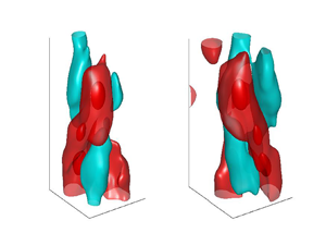
The same events used earlier (i.e.  $\omega _\theta >0$ and
  $\lvert u_\theta \rvert <0.01u_{\theta,max}$) were used to conditionally average the 3-D velocity field at
  $(r_{ref}/d,z_{ref}/d)=(0.82,2.7)$. This location is marked with open square symbols in figures 2(e) and 3(a), where
  $Q3$ events dominate
  $Q1$ events, and positive azimuthal vorticity events are more frequent than negative counterparts. The conditional horseshoe vortex associated with this event is displayed in figure 8 visualized by the swirling strength isosurface
  $\lambda _{ci}=0.22 \lambda _{ci,max}$. Consistent with the instantaneous vortical structures observed in the outer edge of the jet near field shear region, the conditional vortical structure is an upright horseshoe vortex. The leg of this horseshoe vortex is at a
  $50^{\circ }$ angle with respect to the jet centreline, and the distance between the legs, based on the in-plane vector field illustrated in figure 8(c), is approximately
  $0.27d$. Aside from the high-speed region between the head and legs of the conditional horseshoe vortex and the low-speed region above its head, there are two nearly symmetrical low-speed regions on both sides of the horseshoe vortex legs (shown in figure 8c only). These low-speed events are consistent with those on both sides of the vortical structures in the instantaneous flow field presented in figure 4(a). A stagnation line is visible in the in-plane velocity vector field shown in figure 8(b) above the horseshoe vortex head in the streamwise range
  ${\rm \Delta} z/d>2.7$. However, in the streamwise range
  ${\rm \Delta} z/d<2.7$, the mean radial velocity is negative. From this velocity vector field one can conclude that a net flow of fluid from outside of the shear region is induced by the horseshoe vortex into the shear region. This scenario is consistent with the negative mean radial velocity at this location and the positive entrainment of irrotational fluid from outside of the shear region into the turbulent jet. This implies that the large-scale vortical structures are tied to the entrainment in the turbulent jet as suggested by Philip & Marusic (Reference Philip and Marusic2012).

Figure 8. Conditional horseshoe vortex with its head located at  $(r_{ref}/d,z_{ref}/d)=(0.82,2.7)$. The red and cyan isosurfaces show the conditional high-speed and low-speed regions, respectively. (a) Isometric view. (b) Side view with the vector field at
  ${\rm \Delta} x/d=0$. (c) Top view with the vector field at
  ${\rm \Delta} z/d=2.8$. Grey isosurface:
  $\lambda _{ci}=0.22 \lambda _{ci,max}$. Red isosurface:
  $\tilde {u}_z=0.5 \tilde {u}_{z,max}$. Cyan isosurfaces:
  $\tilde {u}_z=0.7 \tilde {u}_{z,min}$ in panels (a) and (b) and
  $\tilde {u}_z=0.3 \tilde {u}_{z,min}$ in panel (c). Events used for conditional averaging are
  $\omega _\theta >0$ and
  $\lvert u_\theta \rvert <0.01u_{\theta,max}$.
The same events used earlier (i.e.  $\omega _\theta >0$ and
  $\lvert u_\theta \rvert <0.01u_{\theta,max}$) were used to conditionally average the 3-D velocity field at
  $(r_{ref}/d,z_{ref}/d)=(2.1,17.4)$ in the jet intermediate field. This location is marked with an open triangle symbol in figures 2(f) and 3(b). The conditional vortical structure associated with this event is displayed in figure 9 using the swirling strength isosurface
  $\lambda _{ci}=0.12 \lambda _{ci,max}$. This is an upright horseshoe vortex, the leg of which is at an approximately
  $40^{\circ }$ angle with respect to the jet centreline. Similar to the conditional horseshoe vortex at the outer edge of the shear region in the jet near field, the conditional horseshoe vortex in the intermediate field induces a negative mean radial velocity, contributing to the entrainment of the irrotational fluid into the turbulent shear region. This is because of the stagnation line in the streamwise range
  ${\rm \Delta} z/d>17.3$ (above the hairpin vortex head), and a negative mean radial velocity in the streamwise range
  ${\rm \Delta} z/d<17.3$ (below the horseshoe vortex head), which are visible in figure 9(b). Based on the velocity vectors in the
  $z\unicode{x2013}y$ plane, the induced negative radial velocity due to the horseshoe vortex in the intermediate field is noticeably smaller than that corresponding to the horseshoe vortex in the jet near field.

Figure 9. Conditional horseshoe vortex with its head located at  $(r_{ref}/d,z_{ref}/d)=(2.1,17.4)$. The red and cyan isosurfaces correspond to the conditional high-speed and low-speed regions, respectively. (a) Isometric view. (b) Side view with the vector field at
  ${\rm \Delta} x/d=0$. (c) Top view with the vector field at
  ${\rm \Delta} z/d=17.5$. Grey isosurface:
  $\lambda _{ci}=0.12 \lambda _{ci,max}$. Red isosurfaces:
 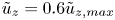 $\tilde {u}_z=0.6 \tilde {u}_{z,max}$. Cyan isosurfaces:
  $\tilde {u}_z=0.8 \tilde {u}_{z,min}$ (in panels a and b) and
  $\tilde {u}_z=0.2 \tilde {u}_{z,min}$ in panel (c). Events used for conditional averaging are
  $\omega _\theta >0$ and
 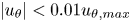 $\lvert u_\theta \rvert <0.01u_{\theta,max}$.
The conditional horseshoe vortices at various streamwise points near the edge of the boundary between the shear region and the potential core in the jet near field were calculated, and their evolution is presented in figure 10. The dashed line represents the jet centreline, while the dotted line denotes the boundary between the shear region and the potential core. It is noted that these conditional vortical structures have been calculated separately, and presented in a single plot for comparison. The conditional vortical structures in this region are inverted horseshoe vortices, and their legs are at a  $30^{\circ}\unicode{x2013}45^{\circ }$ angle with respect to the jet centreline. Moreover, their size appears to remain virtually unchanged with
  $z/d$. This trend is consistent with the nearly constant jet half-radius
  $r_{0.5}$, implying that these large-scale horseshoe vortices probably scale on
  $r_{0.5}$. The jet half-radius is determined as the radial location at which the mean axial velocity is equal to half of the mean axial velocity at the centreline.

Figure 10. Evolution of the conditionally averaged horseshoe vortex close to the potential core in the near field. (a) Isometric view. (b) Side view. (c) Top view. Isosurfaces correspond to  $\lambda _{ci}=0.22 \lambda _{ci,max}$. The dashed line represents the jet centreline, while the dotted line denotes the boundary between the shear region and potential core.
The evolution of horseshoe vortices near the outer edge of the shear region in the jet intermediate field is illustrated in figure 11. Similar to those presented in figure 10, the conditional horseshoe vortices here have been calculated separately, and presented in a single plot for comparison. The  $x$ and
  $y$ axes in figures 11(a) and 11(b) are normalized with the jet diameter
  $d$, while the jet half-radius
  $r_{0.5}$ is used to normalize the
  $x$ and
  $y$ axes in figure 11(c). Evidently, the conditional vortical structures in the jet intermediate field are upright horseshoe vortices and, moving along the streamwise direction, their azimuthal extent increases proportional to
  $r_{0.5}$. Legs of these horseshoe vortices are at an angle in the range
  $35$–
$35$– $45^{\circ }$ with respect to the jet centreline. Comparing the conditional horseshoe vortices in the intermediate field with those in the near field, it is noted that they distinctly differ in shape. Specifically, while the near field conditional vortical structures are horseshoe-shaped structures, those in the intermediate field look like an ‘H’ with shorter upper caps compared with their lower caps. This is highlighted in figure 11(c) by the blue dashed lines. It is probably due to the fact that the conditional vortical structures in the jet intermediate field are formed by both the upright and inverted horseshoe-like vortices. This is because of the weak dominance of
  $Q3$ over
  $Q1$ events near the outer edge of the shear region in the jet intermediate field, which stems from the weak dominance of upright vortical structures over inverted ones in that region. This is one possible explanation for this observation. Alternative valid explanations may exist for this phenomenon.

Figure 11. Evolution of the conditionally averaged horseshoe vortex in the jet intermediate field. (a) Isometric view. (b) Side view. (c) Top view. Isosurfaces correspond to  $\lambda _{ci}=0.11 \lambda _{ci,max}$. The dashed line represents the jet centreline, while the dotted line denotes the boundary between the shear region and outer non-turbulent region. Note that the
  $x$ and
  $y$ axes in panels (a) and (b) are normalized with the jet diameter
  $d$, while the jet half-radius
  $r_{0.5}$ is used to normalize the
  $x$ and
  $y$ axes in panel(c).
The conditional vortical structures presented so far were computed near the boundaries of the shear region with the potential core or the non-turbulent surrounding fluid. According to figure 2, the regions near the boundaries are dominated by either  $Q1$ or
  $Q3$ events. It is proposed that the prevalence of
  $Q1$ or
  $Q3$ events corresponds to one of the two types of horseshoe-like vortex, i.e. an upright or inverted horseshoe vortex. To further illustrate this, the same events used earlier (i.e.
  $\omega _\theta >0$ and
  $\lvert u_\theta \rvert <0.01u_{\theta,max}$) were used to compute the conditional vortical structure at
  $(r_{ref}/d, z_{ref}/d)=(1.3,20.7)$ (marked with a black star in figure 2f), where
  $Q1$ and
  $Q3$ events are in balance. The result, which is displayed in 12(a), is an azimuthally aligned vortex tube (grey isosurface) with no sign of preference for either an upright or inverted horseshoe structure. An induced high-speed region (red isosurface) and an induced low-speed region (cyan isosurface) are also illustrated in figure 12(a). If the constraints
  $u_r>0$ and
  $u_z>0$, i.e. a
  $Q1$ event, are added to the previous conditions at the same location in the flow, an upright conditional horseshoe vortex will be obtained as presented in figure 12(b) in which the red isosurface is a high-speed region corresponding to the conditional streamwise velocity
  $\tilde {u}_z=0.5 \tilde {u}_{z,max}$. On the other hand, if a
  $Q3$ event is applied as the additional constraint, an inverted conditional horseshoe-like vortex is resolved as plotted in figure 12(c). These results clearly demonstrate that, where
  $Q1$ and
  $Q3$ events are in balance, both upright and inverted horseshoe vortices coexist with similar probabilities. They also support the notion that horseshoe vortices correspond closely to
  $Q1$ and
  $Q3$ events and therefore to the entrainment and turbulence production.

Figure 12. Conditional horseshoe vortex with its head located at  $(r_{ref}/d,z_{ref}/d)=(1.3,20.7)$. The red and cyan isosurfaces show the conditional high-speed and low-speed regions, respectively. The condition events are (a)
  $\omega _\theta >0$ and
  $\lvert u_\theta \rvert <0.01u_{\theta,max}$, (b)
  $\omega _\theta >0$,
  $\lvert u_\theta \rvert <0.01u_{\theta,max}$,
  $u_r>0$ and
  $u_z>0$ and (c)
  $\omega _\theta >0$,
  $\lvert u_\theta \rvert <0.01u_{\theta,max}$,
  $u_r<0$ and
  $u_z<0$. Grey isosurface:
  $\lambda _{ci}=0.18 \lambda _{ci,max}$. Red isosurface:
  $\tilde {u}_z=0.5 \tilde {u}_{z,max}$. Cyan isosurface:
 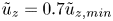 $\tilde {u}_z=0.7 \tilde {u}_{z,min}$.
3.3. Long structures
In the instantaneous flow fields presented in figures 4 and 5, besides horseshoe vortices visualized by the swirling strength, long regions of  $Q1$ and
  $Q3$ are visible. It appears that the high-speed/
 $Q1$ regions, extended in the
  $z$-direction, are induced by the streamwise organization of large-scale horseshoe vortices. Such long structures have been extensively studied in wall-bounded turbulent flows and are referred to as large-scale motions and VLSMs depending on their extension in the streamwise direction (e.g. Hutchins & Marusic Reference Hutchins and Marusic2007; Monty et al. Reference Monty, Stewart, Williams and Chong2007; Lee et al. Reference Lee, Sung and Adrian2019). These structures in wall-bounded flows are low-speed regions, flanked by high-speed regions on either side, and it is believed that they are formed by organized concatenation of large-scale eddy packets (Kevin, Monty & Hutchins Reference Kevin, Monty and Hutchins2019; Lee et al. Reference Lee, Sung and Adrian2019).
Isosurfaces of  $u_z$-fluctuations can be used to visualize these long structures, as shown in figure 13(a), where a sample instantaneous flow field from the jet near field is displayed. To obtain the flow field, the mean streamwise velocity is subtracted to obtain the
  $u_z$-fluctuations, and isosurfaces of
  $u_z=0.1U_j$ (red isosurfaces) and
  $u_z=-0.1U_j$ (cyan isosurfaces) represent the high-speed and low-speed regions, respectively. Isosurfaces with the surface level
  $u_z=0.1U_j$ envelope all the isosurfaces with
  $u_z>0.1U_j$, and similarly isosurfaces with the surface level
  $u_z=-0.1U_j$ encompass all the isosurfaces with
  $u_z<-0.1U_j$. It is worth noting that the overall shapes of the long structures are not overly sensitive to the choice of the isosurface level. Figures 13(b) and 13(c) present isocontours of
  $u_z$-fluctuations on the cross-stream plane
  $z/d=2.8$ and the unwrapped streamwise–azimuthal plane at
  $r/d=0.6$, respectively. Several long streaky high-speed regions flanked by low-speed regions on either side are seen in the 3-D flow field as well as the unwrapped streamwise–azimuthal plane. The length and azimuthal width of these structures increase with
  $z$. The cross-stream
  $u_z$-contours displayed in figure 13(b) exhibit a clear periodic behaviour between the high-speed and low-speed structures in the azimuthal direction; each of these structures spans almost the entire shear region in the radial direction (
 $r/d=0.3\unicode{x2013}1$). In this particular instance, six high-speed and low-speed events are visible in the cross-stream plane at
  $z/d=2.8$. In the majority of cross-stream instances at this streamwise location, four to six high-speed and low-speed events dominate the flow. This is consistent with the findings of Jung et al. (Reference Jung, Gamard and George2004), whose results revealed that, for a round jet, the first POD mode energy distribution peaks at the azimuthal modes
  $m=4\unicode{x2013}6$ in the streamwise range
  $z/d=2\unicode{x2013}3$.

Figure 13. Example instantaneous normalized  $u_z$-fluctuations in the near field. (a) Red isosurface:
  $u_z=0.1U_j$, cyan isosurface:
  $u_z=-0.1U_j$. (b) Contours of normalized
  $u_z$-fluctuations at
  $z/d=2.8$ denoted by a horizontal plane in panel(a). (c) Contours of normalized
  $u_z$-fluctuations on a azimuthal–axial plane at
  $r/d=0.6$. The radial location of this plane is indicated by a circle in panel (b).
Moving on to the intermediate field, an example 3-D instantaneous flow field visualized by isosurfaces of  $u_z$-fluctuations is displayed in figure 14(a). In this plot, the isosurface levels
  $u_z=\pm 0.2U_{cl}$ (where
  $U_{cl}$ is the jet centreline velocity) are chosen for presenting the high-speed and low-speed events. Corresponding 2-D contour maps are plotted in figures 14(b) and 14(c) at the cross-stream plane
  $z/d=21$ and the unwrapped streamwise–azimuthal plane at
  $r/d=1.5$, respectively. A long spiral high-speed region is visible in figure 14(a) extending from
  $z/d=16$ to 27. This is equivalent to an axial length that is
  $\sim$6.7 times the jet half-radius at the centre of this spiral structure. The signature of a 3-D spiral VLSM in an unwrapped streamwise–azimuthal plane is a long structure with an oblique angle relative to the main flow direction. Three such structures are marked with solid lines in figure 14(c). Note that the lines in this figure are for presentation purposes only to highlight the obliqueness of the structures, and are not used in the statistical analysis presented afterwards. An objective detection scheme is presented later (see figure 15). Axisymmetry requires that the probability of occurrences of right-handed and left-handed spirals are equal. In figure 14(c), signatures of both right-handed and left-handed spirals are visible; that is, VLSMs with both negative and positive oblique angles with the main flow direction are present in the flow. Also, seen in this figure is a straight long high-speed event stretching from
  $z/d=15$ to
  $z/d=20$. The long coherent structures appear to extend more than
  $10d$ in the streamwise direction, as seen in figure 14(c), and span between the centreline and the outer edge of the shear region, as it is evident in figure 14(b). Moreover, the cross-stream velocity field corresponds to an azimuthal mode
  $m=2$ in this snapshot, i.e. two high-speed and two low-speed regions. Recently, Samie et al. (Reference Samie, Lavoie and Pollard2021) used two-point velocity measurements, and proposed that an organized concatenation of large-scale structures along the
  $z$-direction results in the formation of spiral VLSMs in the round jet intermediate field. They reached this conclusion based on the configuration of the VLSM component of (two-dimensional) two-point correlation maps. According to Samie et al. (Reference Samie, Lavoie and Pollard2021), these spiral structures consist of high-speed regions flanked on either side by low-speed regions, and are formed by the concatenation of horseshoe vortices. Samie et al. (Reference Samie, Lavoie and Pollard2021) showed that, depending on the radial location, VLSMs constitute between
  $30\,\%$ and
  $80\,\%$ of the total streamwise turbulence intensity in the jet flow. Therefore, VLSMs notably contribute to the dynamics of the jet flow.

Figure 14. Example instantaneous normalized  $u_z$-fluctuations in the fully turbulent region. (a) Red isosurface:
  $u_z=0.2U_{cl}$, cyan isosurface:
  $u_z=-0.2U_{cl}$. (b) Normalized
  $u_z$-fluctuations at
  $z/d=21$ denoted by a horizontal plane on panel (a). (c) Normalized
  $u_z$-fluctuations on an unwrapped azimuthal–axial plane at
  $r/d=1.5$. The radial location of this plane is indicated by the circle in panel (b).

Figure 15. Illustration of the conditional averaging scheme for long coherent structures on an axial–azimuthal plane. (a,b) Two modes of schematic oblique structures. (c) A schematic axially aligned structure.
Instantaneous flow fields such as those presented above reveal long streaky structures in the jet near field and axially aligned and spiral VLSMs in the jet intermediate field. The statistical significance of these coherent features is investigated in greater detail using volumetric conditional averages. The long coherent structures are detected on 2-D streamwise–azimuthal planes using the conditions illustrated in figure 15. Two modes of spiral VLSMs as well as axially aligned VLSMs are detected by this scheme, which relies on a streamwise length ( $l_z$) and an azimuthal length (
 $l_s$) as the input.
The detection scheme was used to conditionally average axially aligned streaky coherent structures in the jet near field ( $z/d=1\unicode{x2013}5$). That is because only these structures were observed in the instantaneous flow field in this region. A 3-D view of the conditional
  $u_z$ flow field around the reference point
  $(z_{ref},r_{ref})=(2.8d,0.6d)$, denoted by
  $\tilde {u}_z$, is displayed in figure 16(a), while corresponding 2-D contour maps on a cross-stream plane at
  $z/d=2.8$ and on an unwrapped streamwise–azimuthal plane at
  $r/d=0.6$ are presented in figures 16(b) and 16(c), respectively. Following the dimensions of the instantaneous streaky structures, the detection input values
  $l_z=d$ and
  $l_s=0.03d$ were used here. Different values of
  $l_z$ and
  $l_s$ were tested to explore the sensitivity of the conditional structure dimensions to the choice of
  $l_z$ and
  $l_s$ (see figure 18 in the Appendix for details). One can see that, while the final conditional velocity field is not sensitive to the value of the azimuthal span
  $l_s$, the length of the main structure increases with increasing
  $l_z$. Nonetheless, this does not affect the qualitative features of the conditional streaky structures. The azimuthal periodicity of the coherent structures, which were observed in the instantaneous flow field, are confirmed by the conditional structure. The
  $\tilde {u}_z$ flow field contains four positive and four negative
  $\tilde {u}_z$ regions corresponding to the azimuthal mode
  $m=4$, implying that the azimuthal mode
  $m=4$ statistically dominates other azimuthal wavenumbers. However, given the superposition of the flow fields associated with all azimuthal wavenumbers in the conditional averaging, structures other than the central structure (located at
  $({\rm \Delta} x/d, {\rm \Delta} y/d)=(0.5, 0)$ in figure 16b) are weak. In addition to the azimuthal periodicity, a streamwise periodicity is implied from figure 16. That is, a negative
  $\tilde {u}_z$ region follows the main positive
  $\tilde {u}_z$ region in the streamwise direction, which is in turn flanked on either side by two positive
  $\tilde {u}_z$ regions. In-plane conditional velocity vectors obtained for a conditional horseshoe vortex in the near field (presented in figure 8) is overlaid on the 2-D contour plots in figure 16(b,c). It is noted that the vector fields are not computed along with the streaky structures using the detection scheme illustrated in figure 15; instead, they correspond to the conditional horseshoe vortex computed in § 3.2 at the same streamwise location. The comparison of the velocity vector field and the
  $\tilde {u}_z$ field reveals that the size of the conditional horseshoe vortex matches that of the conditional streaky structure. This observation lends support to the notion that the streaky structures are induced by 3-D horseshoe vortices that are inclined to the axial direction, rather than purely streamwise vortices.

Figure 16. Conditionally averaged axially aligned streaky structures in the near field based on the conditional scheme illustrated in figure 15(c) with the reference point at  $(z_{ref}, r_{ref})=(2.8d, 0.6d)$. (a) Red isosurfaces:
 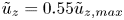 $\tilde {u}_z=0.55\tilde {u}_{z,max}$ and
  $0.12\tilde {u}_{z,max}$ , cyan isosurface:
  $\tilde {u}_z=0.12\tilde {u}_{z,min}$. (b) Contour map of
  $\tilde {u}_z/\tilde {u}_{z,max}$ at
  $z/d=2.8$ denoted by a horizontal plane in panel(a). (c) Contour map of
  $\tilde {u}_z/\tilde {u}_{z,max}$ on a streamwise–azimuthal plane at
  $r/d=0.6$. The radial location of this plane is indicated by the circle in panel (b).
The evidence for the statistical significance of spiral VLSMs is provided here by conditionally averaging these structures using the detection scheme presented in figure 15, after applying a filter to the DNS flow fields that removes small-scale motions. The conditional inputs used for the spiral VLSMs are  $l_z=7d$ and
  $l_s=3d$, and the reference location of the detection is
  $(z_{ref},r_{ref})=(19.7d,1.48d)$. Different combinations of
  $l_z$ and
  $l_s$ were applied to obtain the right-handed spiral (see figure 19 in the Appendix for details). The salient features of the resulting conditional structures remain unchanged for the values of
  $l_z$ and
  $l_s$ considered here, which were chosen upon inspection of several instantaneous flow fields. Three-dimensional views of the conditional VLSMs (two spiral VLSM modes and one axially aligned VLSM) are presented in figure 17(a–c), while corresponding 2-D contour maps on the unwrapped streamwise–azimuthal plane corresponding to the radial location
  $r=1.48d=r_{0.5}$ are displayed in figure 17(d–f). The 3-D structures are visualized by
  $\tilde {u}_z$-isosurfaces, in which conditional high-speed regions correspond to
  $\tilde {u}_z/\tilde {u}_{z,max}=0.1$ and 0.6 (red isosurfaces), and conditional low-speed regions are associated with
  $\tilde {u}_z/\tilde {u}_{z,max}=-0.15$ (cyan isosurfaces). In total, 500 independent flow fields were used for the conditional averaging;
  $34\,\%$ of the total detected VLSMs were right-handed spirals,
  $38\,\%$ were left-handed spirals and
  $28\,\%$ were axially aligned VLSMs. While the percentage contribution from the right-handed and left-handed spirals to the VLSMs are close, they are expected to be equal due to axisymmetry. The observed difference between the percentage for the spiral cases is not statistically significant given the finite number of snapshots available. These percentage contribution values reveal that the spiral VLSMs play a key role in the dynamics of turbulent round jets. The conditional spiral VLSMs are comprised of two high-speed and two low-speed spiral structures, where one high-speed structure is more pronounced than the other one. This is consistent with the azimuthal mode
  $m=2$ in the instantaneous flow fields (figure 14) as well as dominance of the POD eigenspectra (integrated over frequency) at azimuthal modes
  $m=2$ and
  $m=1$ in the jet intermediate and far fields reported in Gamard, Jung & George (Reference Gamard, Jung and George2004). The combination of modes 1 and 2 results in the conditional VLSM displayed in figure 17 in which the second high-speed structure is weak. It can be seen that the long VLSMs constitute three large-scale high-speed features that are aligned diagonally (in spiral VLSMs) or axially (in the axially aligned VLSM) along the
  $z$-direction. The in-plane velocity vector field corresponding to the conditional horseshoe vortex obtained in § 3.2 (see figure 9) is overlaid on the
  $\tilde {u}_z$ contour map depicted in figure 17(d). It is stressed that the velocity vector field has been computed through a separate conditional scheme than the one introduced for the conditional VLSM, and is presented here to compare the conditional horseshoe vortex width with that of the VLSM. The widths of the horseshoe vortex and the spiral VLSM appear to be comparable, promoting the notion that VLSMs are formed by the diagonal concatenation of horseshoe vortices. These 3-D conditional structures are very similar to the conceptual model of spiral VLSMs proposed by Samie et al. (Reference Samie, Lavoie and Pollard2021).

Figure 17. Conditionally averaged VLSMs in the axial range  $z/d=14.5-26.8$ based on the conditional scheme illustrated in figure 15 with the reference point at
  $(z_{ref}, r_{ref})=(19.7d, 1.48d)$. (a–c) Isometric view of VLSMs. The red isosurfaces correspond to
  $\tilde {u}_z/\tilde {u}_{z,max}=0.1$ and 0.6, while the cyan isosurfaces are associated with
  $\tilde {u}_z/\tilde {u}_{z,max}=-0.15$. (d–f) Contour map of
  $\tilde {u}_z/\tilde {u}_{z,max}$ on a streamwise–azimuthal plane at
  $r=r_{ref}$ associated with the (d) right-handed spiral, (e) left-handed spiral and (f) axially aligned VLSM.
4. Concluding remarks
In this paper we used a DNS database from Shin et al. (Reference Shin, Sandberg and Richardson2017) to assess the vortical structures and VLSMs in a turbulent round jet at  $Re_d=7300$. A quadrant analysis applied to the dataset showed that strong
  $Q1$ and
  $Q3$ events, which greatly contribute to the Reynolds shear stress, dominate the turbulent round jet. Further, the analysis revealed that strong
  $Q3$ events dominate the dynamics of the round jet near the outer edge of the shear region in both near and intermediate fields, while strong
  $Q1$ events are more frequent in the shear region close to the potential core in the jet near field. Everywhere else,
  $Q1$ and
  $Q3$ events appear to be in balance. An azimuthal vorticity analysis was also performed on the dataset, which showed that, in the locations where strong
  $Q1$ or
  $Q3$ were dominant, strong positive azimuthal vorticity events prevailed over strong negative counterparts.
Vortex structures in the jet flow fields were visualized using isosurfaces of constant swirling strength, revealing that these structures are frequently present in the turbulent shear regions. Vortical structures in the instantaneous flow fields appeared to be symmetric arch-like as well as asymmetric vortex tubes. It was inferred from instantaneous 3-D flow fields together with the 2-D vector fields that upright horseshoe-like vortex filaments, located near the outer edge of the turbulent shear region, induced regions of  $Q1$ events between their legs and below their heads. These events cause the ejection of high-momentum fluid from the turbulent shear regions to the non-turbulent regions away from the centreline. Moreover,
  $Q3$ events induced above their head entrained non-turbulent fluid into the turbulent shear region. Conversely, inverted horseshoe vortices were frequently present in the turbulent shear region near the potential core (in the jet near field), and induced
  $Q3$ events between their legs and
  $Q1$ events outside of their legs, causing the mixing of the potential core and the turbulent shear region.
The statistical characteristics of vortical structures were assessed by conditional averaging. Informed by the quadrant and azimuthal vorticity sign analyses, physically relevant events were used to obtain conditional volumetric horseshoe vortices by detecting the head of vortex filaments. This yielded a conditional inverted horseshoe vortex in the jet near field in the turbulent shear region near the potential core. Similar conditional averaging revealed upright conditional horseshoe vortices in the jet near and intermediate fields close to the outer edge of the shear region. Moreover, the conditional horseshoe vortices in the intermediate field appeared to be formed by the fusion of upright and inverted vortices with the upright contribution being stronger; this was attributed to the weak dominance of  $Q3$ over
  $Q1$ events in the intermediate field revealed by the quadrant analysis. This suggests that the dominance of upright vortices over the inverted ones near the outer edge of the shear region in the jet intermediate field is weak. It was also shown that dimensions of horseshoe vortices in the near field did not change with the streamwise distance from the jet origin (
 $z$), while the horseshoe vortices in the intermediate field grew in size with the increase in
  $z$.
$z$.
Instantaneous long high-speed regions ( $u_z>0$) flanked on either side by low-speed regions (
 $u_z<0$) were observed in the shear region of the jet near and intermediate fields. They were largely in the form of axially aligned streaky structures in the near field, while in the intermediate field long spiral and axially aligned VLSMs dominated the fluid structures. The positioning of the upright instantaneous horseshoe vortices suggested that these long coherent features were formed by the streamwise grouping of horseshoe vortices. A detection scheme was introduced to detect and average over these long coherent structures. Conditional averaging of these structures in the jet near field resulted in a periodic flow field in both azimuthal and streamwise directions with a dominant azimuthal mode
  $m=4$. Comparing the 2-D velocity vectors corresponding to the conditional near field horseshoe vortex with the conditional large streaky structures indicated that their sizes were identical. This supports the correlation of instantaneous horseshoe vortices and large streaky structures in the near field. The conditionally averaged VLSMs in the jet intermediate field revealed that right-handed and left-handed spiral VLSMs constitute
  $72\,\%$ of the total VLSMs, while the percentage contribution for the axially aligned VLSMs was
  $28\,\%$. Moreover, the conditional spiral and axially aligned VLSMs confirm that the azimuthal mode
  $m=2$ is the dominant azimuthal mode in the jet intermediate field.
Acknowledgements
This collaboration originated from D.S. and A.P. meeting at TSFP-Chicago 2017.
Funding
Financial support of the Natural Sciences and Engineering Research Council of Canada (NSERC) is gratefully acknowledged. This work was supported by the Ministry of Trade, Industry and Energy of the Korean government (20206710100060) and the National Supercomputing Center (KSC-2020-CHA-0006) with supercomputing resources, including technical support.
Declaration of interests
The authors report no conflict of interest.
Appendix
The detection scheme illustrated in figure 15 needs two input parameters, namely, a streamwise dimension denoted by  $l_z$ and an azimuthal dimension given by
  $l_s$. The sensitivity of the conditional structure in the near field is investigated by trying a range of
  $(l_z,l_s)$ combinations, where
  $l_z$ is varied in the range
  $0.5d$–
 $2d$, and
  $l_s$ is changed in the range
  $0.015d$–
 $0.07d$. The values for the pair were chosen based on the dimensions of the instantaneous structures. The effect of
  $l_z$ and
  $l_s$ on the conditional long structures in the near field are presented as conditional streamwise velocity contour maps in figure 18. One can see that
  $l_s$ has minimal effect on the azimuthal span of the conditional structure. However, the streamwise length of the conditional structures increases with increasing
  $l_z$.

Figure 18. Effect of the conditional averaging parameters  $l_z$ and
  $l_s$ on the conditional streaky structure in the jet near field.
Similarly, the sensitivity of the conditional VLSMs in the jet intermediate field to the choice of  $l_z$ and
  $l_s$ was tested by comparing the conditional VLSMs obtained by the detection scheme with various
  $(l_z,l_s)$ pairs as its input. The result is displayed in figure 19. Comparing different conditional VLSMs reveals that changing the input parameters in the range considered here does not affect the salient features of the conditional VLSMs. Note that the values used in this test are chosen based on the dimensions of instantaneous VLSMs.

Figure 19. Effect of the conditional averaging parameters  $l_z$ and
  $l_s$ on the conditional spiral VLSM in the jet intermediate field.


 Open access