


1 Introduction
Quasisymmetry is a type of continuous symmetry in the strength of a toroidal magnetic field
 $B=|\boldsymbol{B}|$
that does not require continuous symmetry of the magnetic field vector
$B=|\boldsymbol{B}|$
that does not require continuous symmetry of the magnetic field vector
 $\boldsymbol{B}$
(Boozer Reference Boozer1983; Nührenberg & Zille Reference Nührenberg and Zille1988; Boozer Reference Boozer1995; Helander Reference Helander2014). As a consequence of the conservation laws associated with quasisymmetry or full axisymmetry of
$\boldsymbol{B}$
(Boozer Reference Boozer1983; Nührenberg & Zille Reference Nührenberg and Zille1988; Boozer Reference Boozer1995; Helander Reference Helander2014). As a consequence of the conservation laws associated with quasisymmetry or full axisymmetry of
 $\boldsymbol{B}$
, both symmetries enable confinement of charged particles and plasma. However, confinement with axisymmetric
$\boldsymbol{B}$
, both symmetries enable confinement of charged particles and plasma. However, confinement with axisymmetric
 $\boldsymbol{B}$
requires a large electric current in the confinement region that is prone to instabilities and hard to sustain, while quasisymmetric confinement does not. Hence, non-axisymmetric toroidal magnetic fields (‘stellarators’) with quasisymmetry offer the promise of stable and efficient confinement of high-temperature plasma for fusion energy. Quasisymmetric stellarators would also enable magnetic confinement of plasmas with density that is too low to support a substantial electric current, such as electron–positron plasmas for basic physics studies (Pedersen et al.
Reference Pedersen, Danielson, Hugenschmidt, Marx, Sarasola, Schauer, Schweikhard, Surko and Winkler2012).
$\boldsymbol{B}$
requires a large electric current in the confinement region that is prone to instabilities and hard to sustain, while quasisymmetric confinement does not. Hence, non-axisymmetric toroidal magnetic fields (‘stellarators’) with quasisymmetry offer the promise of stable and efficient confinement of high-temperature plasma for fusion energy. Quasisymmetric stellarators would also enable magnetic confinement of plasmas with density that is too low to support a substantial electric current, such as electron–positron plasmas for basic physics studies (Pedersen et al.
Reference Pedersen, Danielson, Hugenschmidt, Marx, Sarasola, Schauer, Schweikhard, Surko and Winkler2012).
Several quasisymmetric magnetic field configurations have been found numerically, mostly by using optimization over the space of boundary magnetic surface shapes to minimize symmetry-breaking Fourier modes of
 $B$
(Nührenberg & Zille Reference Nührenberg and Zille1988; Anderson et al.
Reference Anderson, Almagri, Anderson, Matthews, Talmadge and Shohet1995; Garabedian Reference Garabedian1996; Zarnstorff et al.
Reference Zarnstorff, Berry, Brooks, Fredrickson, Fu, Hirshman, Hudson, Ku, Lazarus and Mikkelsen2001; Ku & Boozer Reference Ku and Boozer2011; Drevlak et al.
Reference Drevlak, Brochard, Helander, Kisslinger, Mikhailov, Nührenberg, Nührenberg and Turkin2013; Henneberg et al.
Reference Henneberg, Drevlak, Nührenberg, Beidler, Turkin, Loizu and Helander2019). While this optimization approach is effective, it does not provide much insight into the size and character of the solution space, and it requires good initial guesses for the numerical iteration. Hence, one can never be sure that all the interesting regions of parameter space have been found, for perhaps a different initial guess would yield a new solution. The optimization approach requires significant computation time, and so it is expensive to generate parameterized families of solutions.
$B$
(Nührenberg & Zille Reference Nührenberg and Zille1988; Anderson et al.
Reference Anderson, Almagri, Anderson, Matthews, Talmadge and Shohet1995; Garabedian Reference Garabedian1996; Zarnstorff et al.
Reference Zarnstorff, Berry, Brooks, Fredrickson, Fu, Hirshman, Hudson, Ku, Lazarus and Mikkelsen2001; Ku & Boozer Reference Ku and Boozer2011; Drevlak et al.
Reference Drevlak, Brochard, Helander, Kisslinger, Mikhailov, Nührenberg, Nührenberg and Turkin2013; Henneberg et al.
Reference Henneberg, Drevlak, Nührenberg, Beidler, Turkin, Loizu and Helander2019). While this optimization approach is effective, it does not provide much insight into the size and character of the solution space, and it requires good initial guesses for the numerical iteration. Hence, one can never be sure that all the interesting regions of parameter space have been found, for perhaps a different initial guess would yield a new solution. The optimization approach requires significant computation time, and so it is expensive to generate parameterized families of solutions.
An alternative to the optimization approach is to construct quasisymmetric configurations directly using an analytic expansion, in the smallness of either the departure from axisymmetry of
 $\boldsymbol{B}$
(Plunk & Helander Reference Plunk and Helander2018) or in the distance from the magnetic axis (equivalent to an expansion in large aspect ratio). Near-axis expansions have been explored by several authors (Mercier Reference Mercier1964; Solov’ev & Shafranov Reference Solov’ev and Shafranov1970; Lortz & Nührenberg Reference Lortz and Nührenberg1976), with the particular case of quasisymmetry examined by Garren & Boozer (Reference Garren and Boozer1991a
,Reference Garren and Boozer
b
). The near-axis expansion, although it is an approximation, is always accurate in the core of any stellarator, even stellarators for which the aspect ratio of the outermost surface is not large. In a recent series of papers (Landreman & Sengupta Reference Landreman and Sengupta2018; Landreman, Sengupta & Plunk Reference Landreman, Sengupta and Plunk2019; Plunk, Landreman & Helander Reference Plunk, Landreman and Helander2019), the near-axis expansion was developed into practical procedures for constructing fields with quasisymmetry, or the more general condition of omnigenity. It was also shown that, close to the axis, quasisymmetric configurations obtained by conventional optimization closely match configurations generated by the construction (Landreman Reference Landreman2019). The configurations presented to date from this near-axis construction have been quasisymmetric to first order in
$\boldsymbol{B}$
(Plunk & Helander Reference Plunk and Helander2018) or in the distance from the magnetic axis (equivalent to an expansion in large aspect ratio). Near-axis expansions have been explored by several authors (Mercier Reference Mercier1964; Solov’ev & Shafranov Reference Solov’ev and Shafranov1970; Lortz & Nührenberg Reference Lortz and Nührenberg1976), with the particular case of quasisymmetry examined by Garren & Boozer (Reference Garren and Boozer1991a
,Reference Garren and Boozer
b
). The near-axis expansion, although it is an approximation, is always accurate in the core of any stellarator, even stellarators for which the aspect ratio of the outermost surface is not large. In a recent series of papers (Landreman & Sengupta Reference Landreman and Sengupta2018; Landreman, Sengupta & Plunk Reference Landreman, Sengupta and Plunk2019; Plunk, Landreman & Helander Reference Plunk, Landreman and Helander2019), the near-axis expansion was developed into practical procedures for constructing fields with quasisymmetry, or the more general condition of omnigenity. It was also shown that, close to the axis, quasisymmetric configurations obtained by conventional optimization closely match configurations generated by the construction (Landreman Reference Landreman2019). The configurations presented to date from this near-axis construction have been quasisymmetric to first order in
 $r/{\mathcal{R}}$
, where
$r/{\mathcal{R}}$
, where
 $r$
is the typical distance from the axis and
$r$
is the typical distance from the axis and
 ${\mathcal{R}}$
denotes a scale length of the magnetic axis (such as a typical radius of curvature). At this order, due to regularity conditions at the magnetic axis, the magnetic surfaces must have an elliptical cross-section. It was found that the space of quasisymmetric configurations to this order can be parameterized by the shape of the axis together with three other numbers.
${\mathcal{R}}$
denotes a scale length of the magnetic axis (such as a typical radius of curvature). At this order, due to regularity conditions at the magnetic axis, the magnetic surfaces must have an elliptical cross-section. It was found that the space of quasisymmetric configurations to this order can be parameterized by the shape of the axis together with three other numbers.
In the present paper, we extend the construction to next order in
 $r/{\mathcal{R}}$
. The equations describing quasisymmetry to
$r/{\mathcal{R}}$
. The equations describing quasisymmetry to
 $O((r/{\mathcal{R}})^{2})$
were derived in the appendix of Garren & Boozer (Reference Garren and Boozer1991a
), but no solutions were presented before now. At this order, several important effects appear for the first time, including triangularity and Shafranov shift. By extending the construction to
$O((r/{\mathcal{R}})^{2})$
were derived in the appendix of Garren & Boozer (Reference Garren and Boozer1991a
), but no solutions were presented before now. At this order, several important effects appear for the first time, including triangularity and Shafranov shift. By extending the construction to
 $O((r/{\mathcal{R}})^{2})$
, more complicated and realistic stellarator shapes will be generated, and quasisymmetry will be achieved to higher accuracy. The extension of the model to
$O((r/{\mathcal{R}})^{2})$
, more complicated and realistic stellarator shapes will be generated, and quasisymmetry will be achieved to higher accuracy. The extension of the model to
 $O((r/{\mathcal{R}})^{2})$
only slightly increases the computational cost of solving the equations, which remains on the level of milliseconds on one CPU. This time is far faster than a traditional three-dimensional (3-D) equilibrium calculation, which typically requires of the order of 10 seconds or more.
$O((r/{\mathcal{R}})^{2})$
only slightly increases the computational cost of solving the equations, which remains on the level of milliseconds on one CPU. This time is far faster than a traditional three-dimensional (3-D) equilibrium calculation, which typically requires of the order of 10 seconds or more.
In Garren and Boozer’s original work, it was argued quasisymmetry can be achieved (in the absence of axisymmetry) to
 $O((r/{\mathcal{R}})^{2})$
but not to
$O((r/{\mathcal{R}})^{2})$
but not to
 $O((r/{\mathcal{R}})^{3})$
, so departures from quasisymmetry should scale as the cube of the inverse aspect ratio. However, despite various numerical calculations of quasisymmetric configurations using optimization since 1991, there does not appear to have been a numerical demonstration of this predicted scaling. Using the construction here we are able to numerically demonstrate this predicted ideal scaling for the first time (figure 8). An implication of this scaling is that quasisymmetry can be achieved to arbitrary precision, in the following sense. Given any desired small level of symmetry-breaking Fourier modes in
$O((r/{\mathcal{R}})^{3})$
, so departures from quasisymmetry should scale as the cube of the inverse aspect ratio. However, despite various numerical calculations of quasisymmetric configurations using optimization since 1991, there does not appear to have been a numerical demonstration of this predicted scaling. Using the construction here we are able to numerically demonstrate this predicted ideal scaling for the first time (figure 8). An implication of this scaling is that quasisymmetry can be achieved to arbitrary precision, in the following sense. Given any desired small level of symmetry-breaking Fourier modes in
 $B$
, and given any desired axis shape (constrained only by the requirement that its curvature cannot vanish), there is some aspect ratio above which quasisymmetry can be achieved to the desired precision. To emphasize this point, we will present examples of non-axisymmetric configurations in which quasisymmetry is realized to unprecedented precision, with the symmetry-breaking mode amplitudes orders of magnitude smaller than in previously reported configurations.
$B$
, and given any desired axis shape (constrained only by the requirement that its curvature cannot vanish), there is some aspect ratio above which quasisymmetry can be achieved to the desired precision. To emphasize this point, we will present examples of non-axisymmetric configurations in which quasisymmetry is realized to unprecedented precision, with the symmetry-breaking mode amplitudes orders of magnitude smaller than in previously reported configurations.
A primary application of the work here is to generate input data for stellarator equilibrium codes such as VMEC (Hirshman & Whitson Reference Hirshman and Whitson1983) or optimization codes such as STELLOPT (Spong et al.
Reference Spong, Hirshman, Whitson, Batchelor, Carreras, Lynch and Rome1998; Reiman et al.
Reference Reiman, Fu, Hirshman, Ku, Monticello, Mynick, Redi, Spong, Zarnstorff and Blackwell1999) or ROSE (Drevlak et al.
Reference Drevlak, Beidler, Geiger, Helander and Turkin2019). For these applications, the input we must generate is the shape (or initial shape) of a boundary magnetic surface. In the
 $O(r/{\mathcal{R}})$
construction (Landreman et al.
Reference Landreman, Sengupta and Plunk2019; Plunk et al.
Reference Plunk, Landreman and Helander2019), it was possible to plug a finite value of
$O(r/{\mathcal{R}})$
construction (Landreman et al.
Reference Landreman, Sengupta and Plunk2019; Plunk et al.
Reference Plunk, Landreman and Helander2019), it was possible to plug a finite value of
 $r$
into the near-axis expansion to obtain the boundary surface. In turns out that, at
$r$
into the near-axis expansion to obtain the boundary surface. In turns out that, at
 $O((r/{\mathcal{R}})^{2})$
, this substitution requires some care. We will show that, in fact, a part of the
$O((r/{\mathcal{R}})^{2})$
, this substitution requires some care. We will show that, in fact, a part of the
 $O((r/{\mathcal{R}})^{3})$
shape must be retained in order to generate a boundary surface that is consistent with the desired field strength to
$O((r/{\mathcal{R}})^{3})$
shape must be retained in order to generate a boundary surface that is consistent with the desired field strength to
 $O((r/{\mathcal{R}})^{2})$
. Once this step is taken, we will construct boundary surfaces, then use the VMEC code to generate 3-D equilibria inside the boundaries, and show that quasisymmetry-breaking modes of
$O((r/{\mathcal{R}})^{2})$
. Once this step is taken, we will construct boundary surfaces, then use the VMEC code to generate 3-D equilibria inside the boundaries, and show that quasisymmetry-breaking modes of
 $B$
in these equilibria are small and scale with the aspect ratio, as expected.
$B$
in these equilibria are small and scale with the aspect ratio, as expected.
In the following section, notation will be introduced and the near-axis expansion will be outlined. Section 3 describes the analysis of generating a finite-aspect-ratio boundary surface from the near-axis expansion, and the need for including some
 $O((r/{\mathcal{R}})^{3})$
terms. The numerical method for solving the equations is detailed in § 4, and several examples of constructed quasi-axisymmetric and quasi-helically symmetric configurations are presented in § 5. We discuss the results and conclude in § 6. Several detailed analytic calculations can be found in the appendices. Appendix A gives the equations for
$O((r/{\mathcal{R}})^{3})$
terms. The numerical method for solving the equations is detailed in § 4, and several examples of constructed quasi-axisymmetric and quasi-helically symmetric configurations are presented in § 5. We discuss the results and conclude in § 6. Several detailed analytic calculations can be found in the appendices. Appendix A gives the equations for
 $O((r/{\mathcal{R}})^{2})$
quasisymmetry, derived using a new method that reduces the algebra required. Appendix B gives a detailed proof of results presented in § 3. Finally, one method for converting the constructed boundary shapes to cylindrical coordinates is presented in appendix C.
$O((r/{\mathcal{R}})^{2})$
quasisymmetry, derived using a new method that reduces the algebra required. Appendix B gives a detailed proof of results presented in § 3. Finally, one method for converting the constructed boundary shapes to cylindrical coordinates is presented in appendix C.
2 Near-axis expansion
Our goal is to relate the three-dimensional shapes of flux surfaces to the magnetic field strength in Boozer coordinates
 $(\unicode[STIX]{x1D703},\unicode[STIX]{x1D711})$
. In this section, we introduce the main features of the expansion, and many of the explicit expressions are given in appendix A. While the expansion here is equivalent to the one in Garren & Boozer (Reference Garren and Boozer1991a
,Reference Garren and Boozer
b
), our approach in appendix A provides a streamlined method to derive the equations at each order. Throughout the analysis, we assume that good nested flux surfaces exist in the region of interest near the axis.
$(\unicode[STIX]{x1D703},\unicode[STIX]{x1D711})$
. In this section, we introduce the main features of the expansion, and many of the explicit expressions are given in appendix A. While the expansion here is equivalent to the one in Garren & Boozer (Reference Garren and Boozer1991a
,Reference Garren and Boozer
b
), our approach in appendix A provides a streamlined method to derive the equations at each order. Throughout the analysis, we assume that good nested flux surfaces exist in the region of interest near the axis.
In Boozer coordinates, the magnetic field has the forms
 $$\begin{eqnarray}\displaystyle \boldsymbol{B} & = & \displaystyle \unicode[STIX]{x1D735}\unicode[STIX]{x1D713}\times \unicode[STIX]{x1D735}\unicode[STIX]{x1D703}+\unicode[STIX]{x1D704}\unicode[STIX]{x1D735}\unicode[STIX]{x1D711}\times \unicode[STIX]{x1D735}\unicode[STIX]{x1D713},\nonumber\\ \displaystyle & = & \displaystyle \unicode[STIX]{x1D6FD}\unicode[STIX]{x1D735}\unicode[STIX]{x1D713}+I\unicode[STIX]{x1D735}\unicode[STIX]{x1D703}+G\unicode[STIX]{x1D735}\unicode[STIX]{x1D711},\end{eqnarray}$$
where
 $2\unicode[STIX]{x03C0}\unicode[STIX]{x1D713}$
is the toroidal flux,
$2\unicode[STIX]{x03C0}\unicode[STIX]{x1D713}$
is the toroidal flux,
 $\unicode[STIX]{x1D704}(\unicode[STIX]{x1D713})$
is the rotational transform,
$\unicode[STIX]{x1D704}(\unicode[STIX]{x1D713})$
is the rotational transform,
 $\unicode[STIX]{x1D703}$
and
$\unicode[STIX]{x1D703}$
and
 $\unicode[STIX]{x1D711}$
are the poloidal and toroidal Boozer angles and
$\unicode[STIX]{x1D711}$
are the poloidal and toroidal Boozer angles and
 $I$
and
$I$
and
 $G$
are constant on
$G$
are constant on
 $\unicode[STIX]{x1D713}$
surfaces. To consider quasi-helical symmetry later in the analysis, it is convenient to introduce a helical angle
$\unicode[STIX]{x1D713}$
surfaces. To consider quasi-helical symmetry later in the analysis, it is convenient to introduce a helical angle
 $\unicode[STIX]{x1D717}=\unicode[STIX]{x1D703}-N\unicode[STIX]{x1D711}$
, where
$\unicode[STIX]{x1D717}=\unicode[STIX]{x1D703}-N\unicode[STIX]{x1D711}$
, where
 $N$
is a constant integer. Then
$N$
is a constant integer. Then
 $$\begin{eqnarray}\displaystyle \boldsymbol{B} & = & \displaystyle \unicode[STIX]{x1D735}\unicode[STIX]{x1D713}\times \unicode[STIX]{x1D735}\unicode[STIX]{x1D717}+\unicode[STIX]{x1D704}_{N}\unicode[STIX]{x1D735}\unicode[STIX]{x1D711}\times \unicode[STIX]{x1D735}\unicode[STIX]{x1D713},\end{eqnarray}$$
 $$\begin{eqnarray}\displaystyle & = & \displaystyle \unicode[STIX]{x1D6FD}\unicode[STIX]{x1D735}\unicode[STIX]{x1D713}+I\unicode[STIX]{x1D735}\unicode[STIX]{x1D717}+(G+NI)\unicode[STIX]{x1D735}\unicode[STIX]{x1D711},\end{eqnarray}$$
where
 $\unicode[STIX]{x1D704}_{N}=\unicode[STIX]{x1D704}-N$
.
$\unicode[STIX]{x1D704}_{N}=\unicode[STIX]{x1D704}-N$
.
The position vector
 $\boldsymbol{r}$
at a general point in a neighbourhood of the axis can be described by
$\boldsymbol{r}$
at a general point in a neighbourhood of the axis can be described by
 $$\begin{eqnarray}\boldsymbol{r}(r,\unicode[STIX]{x1D717},\unicode[STIX]{x1D711})=\boldsymbol{r}_{0}(\unicode[STIX]{x1D711})+X(r,\unicode[STIX]{x1D717},\unicode[STIX]{x1D711})\boldsymbol{n}(\unicode[STIX]{x1D711})+Y(r,\unicode[STIX]{x1D717},\unicode[STIX]{x1D711})\boldsymbol{b}(\unicode[STIX]{x1D711})+Z(r,\unicode[STIX]{x1D717},\unicode[STIX]{x1D711})\boldsymbol{t}(\unicode[STIX]{x1D711}),\end{eqnarray}$$
where
 $r$
is the flux surface label defined by
$r$
is the flux surface label defined by
 $2\unicode[STIX]{x03C0}\unicode[STIX]{x1D713}=\unicode[STIX]{x03C0}r^{2}\bar{B}$
, with
$2\unicode[STIX]{x03C0}\unicode[STIX]{x1D713}=\unicode[STIX]{x03C0}r^{2}\bar{B}$
, with
 $\bar{B}$
a constant reference field strength, and
$\bar{B}$
a constant reference field strength, and
 $\boldsymbol{r}_{0}(\unicode[STIX]{x1D711})$
is the position vector along the magnetic axis. Here, the orthonormal vectors
$\boldsymbol{r}_{0}(\unicode[STIX]{x1D711})$
is the position vector along the magnetic axis. Here, the orthonormal vectors
 $(\boldsymbol{t},\boldsymbol{n},\boldsymbol{b})$
give the Frenet–Serret frame of the magnetic axis. These vectors satisfy
$(\boldsymbol{t},\boldsymbol{n},\boldsymbol{b})$
give the Frenet–Serret frame of the magnetic axis. These vectors satisfy
 $$\begin{eqnarray}\frac{\text{d}\unicode[STIX]{x1D711}}{\text{d}\ell }\frac{\text{d}\boldsymbol{r}_{0}}{\text{d}\unicode[STIX]{x1D711}}=\boldsymbol{t},\quad \frac{\text{d}\unicode[STIX]{x1D711}}{\text{d}\ell }\frac{\text{d}\boldsymbol{t}}{\text{d}\unicode[STIX]{x1D711}}=\unicode[STIX]{x1D705}\boldsymbol{n},\quad \frac{\text{d}\unicode[STIX]{x1D711}}{\text{d}\ell }\frac{\text{d}\boldsymbol{n}}{\text{d}\unicode[STIX]{x1D711}}=-\unicode[STIX]{x1D705}\boldsymbol{t}+\unicode[STIX]{x1D70F}\boldsymbol{b},\quad \frac{\text{d}\unicode[STIX]{x1D711}}{\text{d}\ell }\frac{\text{d}\boldsymbol{b}}{\text{d}\unicode[STIX]{x1D711}}=-\unicode[STIX]{x1D70F}\boldsymbol{n},\end{eqnarray}$$
and
 $\boldsymbol{t}\times \boldsymbol{n}=\boldsymbol{b}$
, where
$\boldsymbol{t}\times \boldsymbol{n}=\boldsymbol{b}$
, where
 $\ell$
is the arclength along the axis,
$\ell$
is the arclength along the axis,
 $\unicode[STIX]{x1D705}(\unicode[STIX]{x1D711})$
is the axis curvature and
$\unicode[STIX]{x1D705}(\unicode[STIX]{x1D711})$
is the axis curvature and
 $\unicode[STIX]{x1D70F}(\unicode[STIX]{x1D711})$
is the axis torsion. (Garren and Boozer use the opposite sign convention for torsion.) Using the dual relations,
$\unicode[STIX]{x1D70F}(\unicode[STIX]{x1D711})$
is the axis torsion. (Garren and Boozer use the opposite sign convention for torsion.) Using the dual relations,
 $$\begin{eqnarray}\unicode[STIX]{x1D735}\unicode[STIX]{x1D711}=\frac{1}{\sqrt{g}}\frac{\unicode[STIX]{x2202}\boldsymbol{r}}{\unicode[STIX]{x2202}r}\times \frac{\unicode[STIX]{x2202}\boldsymbol{r}}{\unicode[STIX]{x2202}\unicode[STIX]{x1D717}}\quad \text{and cyclic permutations},\end{eqnarray}$$
where
 $\sqrt{g}=(\unicode[STIX]{x2202}\boldsymbol{r}/\unicode[STIX]{x2202}r)\cdot (\unicode[STIX]{x2202}\boldsymbol{r}/\unicode[STIX]{x2202}\unicode[STIX]{x1D717})\times (\unicode[STIX]{x2202}\boldsymbol{r}/\unicode[STIX]{x2202}\unicode[STIX]{x1D711})$
is the Jacobian, then (2.2)–(2.3) can be expressed in terms of the
$\sqrt{g}=(\unicode[STIX]{x2202}\boldsymbol{r}/\unicode[STIX]{x2202}r)\cdot (\unicode[STIX]{x2202}\boldsymbol{r}/\unicode[STIX]{x2202}\unicode[STIX]{x1D717})\times (\unicode[STIX]{x2202}\boldsymbol{r}/\unicode[STIX]{x2202}\unicode[STIX]{x1D711})$
is the Jacobian, then (2.2)–(2.3) can be expressed in terms of the
 $(\boldsymbol{t},\boldsymbol{n},\boldsymbol{b})$
vectors and derivatives of
$(\boldsymbol{t},\boldsymbol{n},\boldsymbol{b})$
vectors and derivatives of
 $(X,Y,Z)$
. Equating (2.2)–(2.3) then gives three scalar equations, (A 2)–(A 4). The field strength can be expressed in terms of derivatives of
$(X,Y,Z)$
. Equating (2.2)–(2.3) then gives three scalar equations, (A 2)–(A 4). The field strength can be expressed in terms of derivatives of
 $(X,Y,Z)$
using the square of either (2.2) or (2.3). The former turns out to be more useful, and is given in (A 19).
$(X,Y,Z)$
using the square of either (2.2) or (2.3). The former turns out to be more useful, and is given in (A 19).
These equations are supplemented by the equilibrium condition [𝜵 × (2.3) ]× (2.2) =𝜇 0𝜵p, where
 $p(r)$
is the pressure. The average of this condition over
$p(r)$
is the pressure. The average of this condition over
 $\unicode[STIX]{x1D717}$
and
$\unicode[STIX]{x1D717}$
and
 $\unicode[STIX]{x1D711}$
gives
$\unicode[STIX]{x1D711}$
gives
 $$\begin{eqnarray}\frac{\text{d}G}{\text{d}r}+\unicode[STIX]{x1D704}\frac{\text{d}I}{\text{d}r}=-\frac{\unicode[STIX]{x1D707}_{0}}{(2\unicode[STIX]{x03C0})^{2}}(G+\unicode[STIX]{x1D704}I)\frac{\text{d}p}{\text{d}r}\int _{0}^{2\unicode[STIX]{x03C0}}\text{d}\unicode[STIX]{x1D717}\int _{0}^{2\unicode[STIX]{x03C0}}\text{d}\unicode[STIX]{x1D711}\frac{1}{B^{2}},\end{eqnarray}$$
while the
 $\unicode[STIX]{x1D717}$
and
$\unicode[STIX]{x1D717}$
and
 $\unicode[STIX]{x1D711}$
dependence of the equilibrium condition implies
$\unicode[STIX]{x1D711}$
dependence of the equilibrium condition implies
 $$\begin{eqnarray}\frac{\unicode[STIX]{x2202}\unicode[STIX]{x1D6FD}}{\unicode[STIX]{x2202}\unicode[STIX]{x1D711}}+\unicode[STIX]{x1D704}_{N}\frac{\unicode[STIX]{x2202}\unicode[STIX]{x1D6FD}}{\unicode[STIX]{x2202}\unicode[STIX]{x1D717}}=\frac{\unicode[STIX]{x1D707}_{0}}{r\bar{B}}\frac{\text{d}p}{\text{d}r}(G+\unicode[STIX]{x1D704}I)\left[\frac{1}{B^{2}}-\frac{1}{(2\unicode[STIX]{x03C0})^{2}}\int _{0}^{2\unicode[STIX]{x03C0}}\text{d}\unicode[STIX]{x1D717}\int _{0}^{2\unicode[STIX]{x03C0}}\text{d}\unicode[STIX]{x1D711}\frac{1}{B^{2}}\right].\end{eqnarray}$$
The near-axis expansion is then introduced by writing
 $$\begin{eqnarray}X(r,\unicode[STIX]{x1D717},\unicode[STIX]{x1D711})=rX_{1}(\unicode[STIX]{x1D717},\unicode[STIX]{x1D711})+r^{2}X_{2}(\unicode[STIX]{x1D717},\unicode[STIX]{x1D711})+r^{3}X_{3}(\unicode[STIX]{x1D717},\unicode[STIX]{x1D711})+\cdots \,,\end{eqnarray}$$
with analogous expressions for
 $Y$
and
$Y$
and
 $Z$
. Other than
$Z$
. Other than
 $r$
, all scale lengths in the system are ordered as
$r$
, all scale lengths in the system are ordered as
 ${\mathcal{R}}$
, so (2.9) represents an expansion in
${\mathcal{R}}$
, so (2.9) represents an expansion in
 $r/{\mathcal{R}}$
. The field strength is expanded similarly but with an
$r/{\mathcal{R}}$
. The field strength is expanded similarly but with an
 $O((r/{\mathcal{R}})^{0})$
term,
$O((r/{\mathcal{R}})^{0})$
term,
 $$\begin{eqnarray}B(r,\unicode[STIX]{x1D717},\unicode[STIX]{x1D711})=B_{0}(\unicode[STIX]{x1D711})+rB_{1}(\unicode[STIX]{x1D717},\unicode[STIX]{x1D711})+r^{2}B_{2}(\unicode[STIX]{x1D717},\unicode[STIX]{x1D711})+r^{3}B_{3}(\unicode[STIX]{x1D717},\unicode[STIX]{x1D711})+\cdots \,,\end{eqnarray}$$
and
 $\unicode[STIX]{x1D6FD}(r,\unicode[STIX]{x1D717},\unicode[STIX]{x1D711})$
is expanded in the same way. The profile functions
$\unicode[STIX]{x1D6FD}(r,\unicode[STIX]{x1D717},\unicode[STIX]{x1D711})$
is expanded in the same way. The profile functions
 $G(r)$
,
$G(r)$
,
 $I(r)$
,
$I(r)$
,
 $p(r)$
and
$p(r)$
and
 $\unicode[STIX]{x1D704}_{N}(r)$
are analytic functions of
$\unicode[STIX]{x1D704}_{N}(r)$
are analytic functions of
 $\unicode[STIX]{x1D713}$
, so their expansions contain only even powers of
$\unicode[STIX]{x1D713}$
, so their expansions contain only even powers of
 $r$
,
$r$
,
 $$\begin{eqnarray}G(r)=G_{0}+r^{2}G_{2}+r^{4}G_{4}+\cdots \,.\end{eqnarray}$$
Since
 $I(r)$
is proportional to the toroidal current inside the surface
$I(r)$
is proportional to the toroidal current inside the surface
 $r$
, then
$r$
, then
 $I_{0}=0$
. From analyticity considerations near the axis (see appendix A of Landreman & Sengupta (Reference Landreman and Sengupta2018)), the expansion coefficients have the form
$I_{0}=0$
. From analyticity considerations near the axis (see appendix A of Landreman & Sengupta (Reference Landreman and Sengupta2018)), the expansion coefficients have the form
 $$\begin{eqnarray}\left.\begin{array}{@{}rcl@{}}X_{1}(\unicode[STIX]{x1D717},\unicode[STIX]{x1D711})\ & =\ & X_{1s}(\unicode[STIX]{x1D711})\sin (\unicode[STIX]{x1D717})+X_{1c}(\unicode[STIX]{x1D711})\cos (\unicode[STIX]{x1D717}),\\ X_{2}(\unicode[STIX]{x1D717},\unicode[STIX]{x1D711})\ & =\ & X_{20}(\unicode[STIX]{x1D711})+X_{2s}(\unicode[STIX]{x1D711})\sin (2\unicode[STIX]{x1D717})+X_{2c}(\unicode[STIX]{x1D711})\cos (2\unicode[STIX]{x1D717}),\\ X_{3}(\unicode[STIX]{x1D717},\unicode[STIX]{x1D711})\ & =\ & X_{3s3}(\unicode[STIX]{x1D711})\sin (3\unicode[STIX]{x1D717})+X_{3s1}(\unicode[STIX]{x1D711})\sin (\unicode[STIX]{x1D717})+X_{3c3}(\unicode[STIX]{x1D711})\cos (3\unicode[STIX]{x1D717})+X_{3c1}(\unicode[STIX]{x1D711})\cos (\unicode[STIX]{x1D717}).\end{array}\right\}\end{eqnarray}$$
The expansions of
 $Y$
,
$Y$
,
 $Z$
,
$Z$
,
 $B$
and
$B$
and
 $\unicode[STIX]{x1D6FD}$
have the same form. The expansions (2.9)–(2.12) are then substituted into (A 2)–(A 4), (A 19) and (2.7)–(2.8), and terms at each order in
$\unicode[STIX]{x1D6FD}$
have the same form. The expansions (2.9)–(2.12) are then substituted into (A 2)–(A 4), (A 19) and (2.7)–(2.8), and terms at each order in
 $r/{\mathcal{R}}$
are collected. We can thereby relate the surface shape coefficients
$r/{\mathcal{R}}$
are collected. We can thereby relate the surface shape coefficients
 $(X,Y,Z)$
to the field strength through a desired order in
$(X,Y,Z)$
to the field strength through a desired order in
 $r/{\mathcal{R}}$
. Explicit results through
$r/{\mathcal{R}}$
. Explicit results through
 $O((r/{\mathcal{R}})^{2})$
are given in (A 20)–(A 52).
$O((r/{\mathcal{R}})^{2})$
are given in (A 20)–(A 52).
Quasisymmetry is achieved through order
 $O((r/{\mathcal{R}})^{j})$
when
$O((r/{\mathcal{R}})^{j})$
when
 $\unicode[STIX]{x2202}B_{k}/\unicode[STIX]{x2202}\unicode[STIX]{x1D711}=0$
for
$\unicode[STIX]{x2202}B_{k}/\unicode[STIX]{x2202}\unicode[STIX]{x1D711}=0$
for
 $k\leqslant \,j$
. At
$k\leqslant \,j$
. At
 $O((r/{\mathcal{R}})^{1})$
, the analysis in appendix A shows quasisymmetric fields are described by
$O((r/{\mathcal{R}})^{1})$
, the analysis in appendix A shows quasisymmetric fields are described by
 $$\begin{eqnarray}\boldsymbol{r}(r,\unicode[STIX]{x1D717},\unicode[STIX]{x1D711})=\boldsymbol{r}_{0}(\unicode[STIX]{x1D711})+\frac{r\bar{\unicode[STIX]{x1D702}}}{\unicode[STIX]{x1D705}(\unicode[STIX]{x1D711})}\cos \unicode[STIX]{x1D717}\boldsymbol{n}(\unicode[STIX]{x1D711})+\frac{rs_{\unicode[STIX]{x1D713}}s_{G}\unicode[STIX]{x1D705}(\unicode[STIX]{x1D711})}{\bar{\unicode[STIX]{x1D702}}}\left[\sin \unicode[STIX]{x1D717}+\unicode[STIX]{x1D70E}(\unicode[STIX]{x1D711})\cos \unicode[STIX]{x1D717}\right]\boldsymbol{b}(\unicode[STIX]{x1D711})+O(r^{2}/{\mathcal{R}}),\end{eqnarray}$$
where
 $s_{\unicode[STIX]{x1D713}}=\text{sign}(\unicode[STIX]{x1D713})$
,
$s_{\unicode[STIX]{x1D713}}=\text{sign}(\unicode[STIX]{x1D713})$
,
 $s_{G}=\text{sign}(G_{0})$
,
$s_{G}=\text{sign}(G_{0})$
,
 $\bar{\unicode[STIX]{x1D702}}$
is a constant and
$\bar{\unicode[STIX]{x1D702}}$
is a constant and
 $\unicode[STIX]{x1D70E}(\unicode[STIX]{x1D711})$
is a solution of
$\unicode[STIX]{x1D70E}(\unicode[STIX]{x1D711})$
is a solution of
 $$\begin{eqnarray}\frac{\text{d}\unicode[STIX]{x1D70E}}{\text{d}\unicode[STIX]{x1D711}}+(\unicode[STIX]{x1D704}_{0}-N)\left[\frac{\bar{\unicode[STIX]{x1D702}}^{4}}{\unicode[STIX]{x1D705}^{4}}+1+\unicode[STIX]{x1D70E}^{2}\right]-\frac{2G_{0}\bar{\unicode[STIX]{x1D702}}^{2}}{B_{0}\unicode[STIX]{x1D705}^{2}}\left[\frac{I_{2}}{B_{0}}-s_{\unicode[STIX]{x1D713}}\unicode[STIX]{x1D70F}\right]=0.\end{eqnarray}$$
Here, the constant
 $I_{2}$
is the leading term in the coefficient
$I_{2}$
is the leading term in the coefficient
 $I(r)$
of (2.1), and is proportional to the on-axis toroidal current density, which is typically zero. The constant
$I(r)$
of (2.1), and is proportional to the on-axis toroidal current density, which is typically zero. The constant
 $\bar{\unicode[STIX]{x1D702}}=B_{1c}/B_{0}$
(introduced by Garren & Boozer (Reference Garren and Boozer1991b
)) reflects the magnitude by which
$\bar{\unicode[STIX]{x1D702}}=B_{1c}/B_{0}$
(introduced by Garren & Boozer (Reference Garren and Boozer1991b
)) reflects the magnitude by which
 $B$
varies on surfaces,
$B$
varies on surfaces,
 $$\begin{eqnarray}B\approx B_{0}[1+r\bar{\unicode[STIX]{x1D702}}\cos \unicode[STIX]{x1D717}+O((r/{\mathcal{R}})^{2})].\end{eqnarray}$$
The surface shapes corresponding to (2.13) are ellipses in the plane perpendicular to the axis (the
 $\boldsymbol{n}$
–
$\boldsymbol{n}$
–
 $\boldsymbol{b}$
plane). The ellipses are centred on the magnetic axis, so there is no Shafranov shift to this order.
$\boldsymbol{b}$
plane). The ellipses are centred on the magnetic axis, so there is no Shafranov shift to this order.
It can be proved (Landreman et al.
Reference Landreman, Sengupta and Plunk2019) that quasisymmetric fields to
 $O(r/{\mathcal{R}})$
can be parameterized by the shape of the axis – which can be any curve for which
$O(r/{\mathcal{R}})$
can be parameterized by the shape of the axis – which can be any curve for which
 $\unicode[STIX]{x1D705}$
never vanishes – along with three real numbers:
$\unicode[STIX]{x1D705}$
never vanishes – along with three real numbers:
 $I_{2}$
,
$I_{2}$
,
 $\bar{\unicode[STIX]{x1D702}}$
and
$\bar{\unicode[STIX]{x1D702}}$
and
 $\unicode[STIX]{x1D70E}(0)$
. Varying
$\unicode[STIX]{x1D70E}(0)$
. Varying
 $\bar{\unicode[STIX]{x1D702}}$
has the effect of varying the average elongation. The parameter
$\bar{\unicode[STIX]{x1D702}}$
has the effect of varying the average elongation. The parameter
 $\unicode[STIX]{x1D70E}(0)$
is the value of
$\unicode[STIX]{x1D70E}(0)$
is the value of
 $\unicode[STIX]{x1D70E}(\unicode[STIX]{x1D711})$
at
$\unicode[STIX]{x1D70E}(\unicode[STIX]{x1D711})$
at
 $\unicode[STIX]{x1D711}=0$
, and it reflects the angle by which the major and minor axes of the elliptical flux surfaces are oriented with respect to
$\unicode[STIX]{x1D711}=0$
, and it reflects the angle by which the major and minor axes of the elliptical flux surfaces are oriented with respect to
 $\boldsymbol{n}$
at
$\boldsymbol{n}$
at
 $\unicode[STIX]{x1D711}=0$
. Stellarators typically possess ‘stellarator symmetry’ (unrelated to quasisymmetry) which implies
$\unicode[STIX]{x1D711}=0$
. Stellarators typically possess ‘stellarator symmetry’ (unrelated to quasisymmetry) which implies
 $\unicode[STIX]{x1D70E}(0)=0$
. The pressure profile does not appear in the model to this order.
$\unicode[STIX]{x1D70E}(0)=0$
. The pressure profile does not appear in the model to this order.
Proceeding to
 $O((r/{\mathcal{R}})^{2})$
, nine new functions of
$O((r/{\mathcal{R}})^{2})$
, nine new functions of
 $\unicode[STIX]{x1D711}$
arise in the surface shapes:
$\unicode[STIX]{x1D711}$
arise in the surface shapes:
 $X_{20}$
,
$X_{20}$
,
 $X_{2s}$
,
$X_{2s}$
,
 $X_{2c}$
,
$X_{2c}$
,
 $Y_{20}$
,
$Y_{20}$
,
 $Y_{2s}$
,
$Y_{2s}$
,
 $Y_{2c}$
,
$Y_{2c}$
,
 $Z_{20}$
,
$Z_{20}$
,
 $Z_{2s}$
and
$Z_{2s}$
and
 $Z_{2c}$
. The corresponding surface shapes can now possess triangularity, and
$Z_{2c}$
. The corresponding surface shapes can now possess triangularity, and
 $X_{20}$
and
$X_{20}$
and
 $Y_{20}$
enable the centre of the surfaces at any given
$Y_{20}$
enable the centre of the surfaces at any given
 $(r,\unicode[STIX]{x1D711})$
to be shifted in the
$(r,\unicode[STIX]{x1D711})$
to be shifted in the
 $\boldsymbol{n}$
–
$\boldsymbol{n}$
–
 $\boldsymbol{b}$
plane with respect to the axis (Shafranov shift). These nine functions are constrained by 10 new
$\boldsymbol{b}$
plane with respect to the axis (Shafranov shift). These nine functions are constrained by 10 new
 $\unicode[STIX]{x1D711}$
-dependent equations: (A 27)–(A 29), (A 32)–(A 36) and (A 41)–(A 42) (with
$\unicode[STIX]{x1D711}$
-dependent equations: (A 27)–(A 29), (A 32)–(A 36) and (A 41)–(A 42) (with
 $X_{1s}=\unicode[STIX]{x1D6FD}_{0}=\unicode[STIX]{x1D6FD}_{1c}=0$
as explained in A.3). Therefore, as noted by Garren & Boozer (Reference Garren and Boozer1991b
,Reference Garren and Boozer
a
), there is a net loss of one
$X_{1s}=\unicode[STIX]{x1D6FD}_{0}=\unicode[STIX]{x1D6FD}_{1c}=0$
as explained in A.3). Therefore, as noted by Garren & Boozer (Reference Garren and Boozer1991b
,Reference Garren and Boozer
a
), there is a net loss of one
 $\unicode[STIX]{x1D711}$
-dependent degree of freedom, and so most axis shapes are not consistent with quasisymmetry through this order, in contrast to the
$\unicode[STIX]{x1D711}$
-dependent degree of freedom, and so most axis shapes are not consistent with quasisymmetry through this order, in contrast to the
 $O(r/{\mathcal{R}})$
case.
$O(r/{\mathcal{R}})$
case.
Also, four new scalar parameters appear at
 $O((r/{\mathcal{R}})^{2})$
that are independent of
$O((r/{\mathcal{R}})^{2})$
that are independent of
 $\unicode[STIX]{x1D711}$
. One is
$\unicode[STIX]{x1D711}$
. One is
 $p_{2}$
, providing the first information about the pressure profile. Also appearing are the numbers
$p_{2}$
, providing the first information about the pressure profile. Also appearing are the numbers
 $B_{20}$
,
$B_{20}$
,
 $B_{2s}$
and
$B_{2s}$
and
 $B_{2c}$
, describing the variation of
$B_{2c}$
, describing the variation of
 $B$
with
$B$
with
 $\unicode[STIX]{x1D717}$
. The global magnetic shear does not yet enter the system of equations; it first appears at
$\unicode[STIX]{x1D717}$
. The global magnetic shear does not yet enter the system of equations; it first appears at
 $O((r/{\mathcal{R}})^{3})$
.
$O((r/{\mathcal{R}})^{3})$
.
3 Generating a finite-minor-radius boundary
Our goal is ultimately to construct the shape of a boundary magnetic surface such that the magnetic field in the interior is quasisymmetric to a good approximation. The interest in constructing boundary surfaces comes from the fact that magnetohydrodynamic (MHD) equilibrium codes such as VMEC naturally take the shape of a boundary magnetic surface as an input. Conventional stellarator optimization codes such as STELLOPT and ROSE are built upon VMEC, so if we can construct a boundary surface for a quasisymmetric configuration, then we can construct a good initial condition for optimization.
Given a solution of the equations of the near-axis expansion through some order, how can a boundary surface be generated? A natural approach is to plug a small but finite value
 $a$
of the expansion parameter
$a$
of the expansion parameter
 $r$
into the series for
$r$
into the series for
 $(X,Y,Z)$
, which yields a toroidal surface with average minor radius
$(X,Y,Z)$
, which yields a toroidal surface with average minor radius
 $a$
. This approach was applied successfully to the
$a$
. This approach was applied successfully to the
 $O((r/{\mathcal{R}})^{1})$
equations in Landreman et al. (Reference Landreman, Sengupta and Plunk2019) and Plunk et al. (Reference Plunk, Landreman and Helander2019). However, this approach of setting
$O((r/{\mathcal{R}})^{1})$
equations in Landreman et al. (Reference Landreman, Sengupta and Plunk2019) and Plunk et al. (Reference Plunk, Landreman and Helander2019). However, this approach of setting
 $r\rightarrow a$
turns out to require modification when applied to the
$r\rightarrow a$
turns out to require modification when applied to the
 $O((r/{\mathcal{R}})^{2})$
equations. It can be seen that some care is required when setting
$O((r/{\mathcal{R}})^{2})$
equations. It can be seen that some care is required when setting
 $r$
to a finite value, as follows. When the expansion is truncated at a finite order in
$r$
to a finite value, as follows. When the expansion is truncated at a finite order in
 $r/{\mathcal{R}}$
, a finite value of
$r/{\mathcal{R}}$
, a finite value of
 $r$
chosen and MHD equilibrium computed within the resulting surface, a configuration results that has a slightly different axis shape and
$r$
chosen and MHD equilibrium computed within the resulting surface, a configuration results that has a slightly different axis shape and
 $(X,Y,Z)$
coefficients than the ones assumed in the original expansion. The difference turns out to be unimportant for the
$(X,Y,Z)$
coefficients than the ones assumed in the original expansion. The difference turns out to be unimportant for the
 $O((r/{\mathcal{R}})^{1})$
construction but critical for the
$O((r/{\mathcal{R}})^{1})$
construction but critical for the
 $O((r/{\mathcal{R}})^{2})$
construction. The fact that plugging in a finite value of
$O((r/{\mathcal{R}})^{2})$
construction. The fact that plugging in a finite value of
 $r$
to obtain a boundary results in a slight change to the equilibrium can be seen in figures 3, 8 and 10 of Landreman et al. (Reference Landreman, Sengupta and Plunk2019). These figures, showing the
$r$
to obtain a boundary results in a slight change to the equilibrium can be seen in figures 3, 8 and 10 of Landreman et al. (Reference Landreman, Sengupta and Plunk2019). These figures, showing the
 $B$
spectrum when a finite
$B$
spectrum when a finite
 $r$
is substituted into the
$r$
is substituted into the
 $O((r/{\mathcal{R}})^{1})$
Garren–Boozer expansion and the equilibrium is computed inside the resulting boundary, show that there is a small but finite mirror mode on the magnetic axis, even though the on-axis mirror mode amplitude is precisely zero in the original expansion.
$O((r/{\mathcal{R}})^{1})$
Garren–Boozer expansion and the equilibrium is computed inside the resulting boundary, show that there is a small but finite mirror mode on the magnetic axis, even though the on-axis mirror mode amplitude is precisely zero in the original expansion.
In this section, we introduce a systematic method to examine the effect of setting the expansion parameter
 $r$
equal to a finite number
$r$
equal to a finite number
 $a$
. Technical details of the calculation are given in appendix B. Here, and in the appendix, we consider a more general problem of trying to construct a configuration with any desired field strength
$a$
. Technical details of the calculation are given in appendix B. Here, and in the appendix, we consider a more general problem of trying to construct a configuration with any desired field strength
 $B(r,\unicode[STIX]{x1D717},\unicode[STIX]{x1D711})$
, which may or may not be quasisymmetric; therefore, the analysis also applies to more general optimizations such as omnigenity. The basic approach is to introduce a second Garren–Boozer-type expansion, denoted with tildes, that describes the configuration which results from computing an MHD equilibrium inside the boundary constructed from the original Garren–Boozer expansion. In contrast to the original expansion, the ‘tilde’ expansion is not truncated, since it describes MHD equilibrium in a finite volume. The axis shapes and
$B(r,\unicode[STIX]{x1D717},\unicode[STIX]{x1D711})$
, which may or may not be quasisymmetric; therefore, the analysis also applies to more general optimizations such as omnigenity. The basic approach is to introduce a second Garren–Boozer-type expansion, denoted with tildes, that describes the configuration which results from computing an MHD equilibrium inside the boundary constructed from the original Garren–Boozer expansion. In contrast to the original expansion, the ‘tilde’ expansion is not truncated, since it describes MHD equilibrium in a finite volume. The axis shapes and
 $(X,Y,Z)$
coefficients for the tilde and non-tilde expansions are similar but not identical. Their differences diminish as
$(X,Y,Z)$
coefficients for the tilde and non-tilde expansions are similar but not identical. Their differences diminish as
 $a\rightarrow 0$
. The non-tilde expansion represents a single idealized configuration we would like to achieve, whereas the tilde expansion represents a family of different ‘real’ configurations, (real in the sense that they are what is computed by solving for MHD equilibrium without a near-axis expansion), parameterized by the finite value
$a\rightarrow 0$
. The non-tilde expansion represents a single idealized configuration we would like to achieve, whereas the tilde expansion represents a family of different ‘real’ configurations, (real in the sense that they are what is computed by solving for MHD equilibrium without a near-axis expansion), parameterized by the finite value
 $a$
used to construct their boundaries. From the fact that the (truncated) non-tilde expansion and (non-truncated) tilde expansions describe the same surface at
$a$
used to construct their boundaries. From the fact that the (truncated) non-tilde expansion and (non-truncated) tilde expansions describe the same surface at
 $r=a$
, and exploiting an expansion in
$r=a$
, and exploiting an expansion in
 $r/{\mathcal{R}}\ll 1$
with the ordering
$r/{\mathcal{R}}\ll 1$
with the ordering
 $a\sim r$
, we can derive the magnetic field strength that results for the constructed configurations. We will thereby rigorously show that substituting
$a\sim r$
, we can derive the magnetic field strength that results for the constructed configurations. We will thereby rigorously show that substituting
 $r\rightarrow a$
in an
$r\rightarrow a$
in an
 $O(r/{\mathcal{R}})$
Garren–Boozer solution yields a configuration that has the desired
$O(r/{\mathcal{R}})$
Garren–Boozer solution yields a configuration that has the desired
 $B$
to
$B$
to
 $O(r/{\mathcal{R}})$
, but substituting
$O(r/{\mathcal{R}})$
, but substituting
 $r\rightarrow a$
in an
$r\rightarrow a$
in an
 $O((r/{\mathcal{R}})^{2})$
Garren–Boozer solution yields a configuration that only has the desired
$O((r/{\mathcal{R}})^{2})$
Garren–Boozer solution yields a configuration that only has the desired
 $B$
through
$B$
through
 $O(r/{\mathcal{R}})$
, not
$O(r/{\mathcal{R}})$
, not
 $O((r/{\mathcal{R}})^{2})$
. However, the achieved
$O((r/{\mathcal{R}})^{2})$
. However, the achieved
 $B$
can be made to match the desired one at
$B$
can be made to match the desired one at
 $O((r/{\mathcal{R}})^{2})$
by a small modification of the construction, in which
$O((r/{\mathcal{R}})^{2})$
by a small modification of the construction, in which
 $X_{3}$
and
$X_{3}$
and
 $Y_{3}$
terms are included.
$Y_{3}$
terms are included.
Beginning the formal analysis, we consider a family of equilibria parameterized by
 $a$
, in which the position vector is
$a$
, in which the position vector is
 $$\begin{eqnarray}\boldsymbol{r}=\tilde{\boldsymbol{r}}_{0}(a,\tilde{\unicode[STIX]{x1D711}})+\tilde{X}(a,r,\tilde{\unicode[STIX]{x1D717}},\tilde{\unicode[STIX]{x1D711}})\tilde{\boldsymbol{n}}(a,\tilde{\unicode[STIX]{x1D711}})+{\tilde{Y}}(a,r,\tilde{\unicode[STIX]{x1D717}},\tilde{\unicode[STIX]{x1D711}})\tilde{\boldsymbol{b}}(a,\tilde{\unicode[STIX]{x1D711}})+\tilde{Z}(a,r,\tilde{\unicode[STIX]{x1D717}},\tilde{\unicode[STIX]{x1D711}})\tilde{\boldsymbol{t}}(a,\tilde{\unicode[STIX]{x1D711}}),\end{eqnarray}$$
analogous to (2.4). The Boozer angles
 $(\tilde{\unicode[STIX]{x1D717}},\tilde{\unicode[STIX]{x1D711}})$
for the real configuration generally differ somewhat from the angles
$(\tilde{\unicode[STIX]{x1D717}},\tilde{\unicode[STIX]{x1D711}})$
for the real configuration generally differ somewhat from the angles
 $(\unicode[STIX]{x1D717},\unicode[STIX]{x1D711})$
of the ideal configuration, with the differences denoted by single-valued functions
$(\unicode[STIX]{x1D717},\unicode[STIX]{x1D711})$
of the ideal configuration, with the differences denoted by single-valued functions
 $t$
and
$t$
and
 $f$
,
$f$
,
 $$\begin{eqnarray}\tilde{\unicode[STIX]{x1D717}}(a,\unicode[STIX]{x1D717},\unicode[STIX]{x1D711})=\unicode[STIX]{x1D717}+t(a,\unicode[STIX]{x1D717},\unicode[STIX]{x1D711}),\quad \tilde{\unicode[STIX]{x1D711}}(a,\unicode[STIX]{x1D717},\unicode[STIX]{x1D711})=\unicode[STIX]{x1D711}+f(a,\unicode[STIX]{x1D717},\unicode[STIX]{x1D711}).\end{eqnarray}$$
Analogous to (2.9), we have
 $$\begin{eqnarray}\tilde{X}(a,r,\tilde{\unicode[STIX]{x1D717}},\tilde{\unicode[STIX]{x1D711}})=\mathop{\sum }_{j=1}^{\infty }r^{\,j}\tilde{X}_{j}(a,\tilde{\unicode[STIX]{x1D717}},\tilde{\unicode[STIX]{x1D711}}),\end{eqnarray}$$
with similar expansions for
 ${\tilde{Y}}$
and
${\tilde{Y}}$
and
 $\tilde{Z}$
, and analogous to (2.9), the field strength in the real configurations is
$\tilde{Z}$
, and analogous to (2.9), the field strength in the real configurations is
 $$\begin{eqnarray}\tilde{B}(a,r,\tilde{\unicode[STIX]{x1D717}},\tilde{\unicode[STIX]{x1D711}})=\mathop{\sum }_{j=0}^{\infty }r^{\,j}\tilde{B}_{j}(a,\tilde{\unicode[STIX]{x1D717}},\tilde{\unicode[STIX]{x1D711}}),\end{eqnarray}$$
with a similar expansion for
 $\tilde{\unicode[STIX]{x1D6FD}}$
. All quantities in the tilde configurations are assumed to have
$\tilde{\unicode[STIX]{x1D6FD}}$
. All quantities in the tilde configurations are assumed to have
 $a$
-dependence in the form of a Taylor series, with coefficients denoted by superscripts in parentheses,
$a$
-dependence in the form of a Taylor series, with coefficients denoted by superscripts in parentheses,
 $$\begin{eqnarray}\tilde{\boldsymbol{r}}_{0}(a,\tilde{\unicode[STIX]{x1D711}})=\mathop{\sum }_{k=0}^{\infty }a^{k}\tilde{\boldsymbol{r}}_{0}^{(k)}(\tilde{\unicode[STIX]{x1D711}}),\end{eqnarray}$$
with analogous expansions for
 $\tilde{\boldsymbol{n}}$
,
$\tilde{\boldsymbol{n}}$
,
 $\tilde{\boldsymbol{b}}$
and
$\tilde{\boldsymbol{b}}$
and
 $\tilde{\boldsymbol{t}}$
, and
$\tilde{\boldsymbol{t}}$
, and
 $$\begin{eqnarray}\tilde{X}_{j}(a,\tilde{\unicode[STIX]{x1D717}},\tilde{\unicode[STIX]{x1D711}})=\mathop{\sum }_{k=0}^{\infty }a^{k}\tilde{X}_{j}^{(k)}(\tilde{\unicode[STIX]{x1D717}},\tilde{\unicode[STIX]{x1D711}}),\end{eqnarray}$$
with analogous expansions for
 ${\tilde{Y}}_{j}$
,
${\tilde{Y}}_{j}$
,
 $\tilde{Z}_{j}$
,
$\tilde{Z}_{j}$
,
 $\tilde{B}_{j}$
and
$\tilde{B}_{j}$
and
 $\tilde{\unicode[STIX]{x1D6FD}}_{j}$
. We similarly assume
$\tilde{\unicode[STIX]{x1D6FD}}_{j}$
. We similarly assume
 $$\begin{eqnarray}t(a,\unicode[STIX]{x1D717},\unicode[STIX]{x1D711})=\mathop{\sum }_{k=0}^{\infty }a^{k}t^{(k)}(\unicode[STIX]{x1D717},\unicode[STIX]{x1D711}),\quad f(a,\unicode[STIX]{x1D717},\unicode[STIX]{x1D711})=\mathop{\sum }_{k=0}^{\infty }a^{k}f^{(k)}(\unicode[STIX]{x1D717},\unicode[STIX]{x1D711}).\end{eqnarray}$$
To reiterate, subscripts refer to an expansion in distance from the axis in a fixed configuration, whereas superscripts in parentheses indicate a distinct expansion in the finite value of minor radius substituted into the original near-axis expansion.
The boundary of a tilde configuration, i.e. its
 $r=a$
surface, by definition is the surface obtained by setting
$r=a$
surface, by definition is the surface obtained by setting
 $r=a$
in the non-tilde expansion. The equation representing this fact is
$r=a$
in the non-tilde expansion. The equation representing this fact is
 $$\begin{eqnarray}\displaystyle & & \displaystyle \boldsymbol{r}_{0}(\unicode[STIX]{x1D711})+X(a,\unicode[STIX]{x1D717},\unicode[STIX]{x1D711})\boldsymbol{n}(\unicode[STIX]{x1D711})+Y(a,\unicode[STIX]{x1D717},\unicode[STIX]{x1D711})\boldsymbol{b}(\unicode[STIX]{x1D711})+Z(a,\unicode[STIX]{x1D717},\unicode[STIX]{x1D711})\boldsymbol{t}(\unicode[STIX]{x1D711})\nonumber\\ \displaystyle & & \displaystyle \quad =\tilde{\boldsymbol{r}}_{0}(a,\tilde{\unicode[STIX]{x1D711}})+\tilde{X}(a,a,\tilde{\unicode[STIX]{x1D717}},\tilde{\unicode[STIX]{x1D711}})\tilde{\boldsymbol{n}}(a,\tilde{\unicode[STIX]{x1D711}})+{\tilde{Y}}(a,a,\tilde{\unicode[STIX]{x1D717}},\tilde{\unicode[STIX]{x1D711}})\tilde{\boldsymbol{b}}(a,\tilde{\unicode[STIX]{x1D711}})\nonumber\\ \displaystyle & & \displaystyle \qquad +\,\tilde{Z}(a,a,\tilde{\unicode[STIX]{x1D717}},\tilde{\unicode[STIX]{x1D711}})\tilde{\boldsymbol{t}}(a,\tilde{\unicode[STIX]{x1D711}}),\end{eqnarray}$$
and it plays a central role in the analysis.
To the order of interest, the field strength in the real configurations is
 $$\begin{eqnarray}\displaystyle \tilde{B}(a,r,\tilde{\unicode[STIX]{x1D717}},\tilde{\unicode[STIX]{x1D711}}) & = & \displaystyle \tilde{B}_{0}^{(0)}(\tilde{\unicode[STIX]{x1D711}})+r\tilde{B}_{1}^{(0)}(\tilde{\unicode[STIX]{x1D717}},\tilde{\unicode[STIX]{x1D711}})+a\tilde{B}_{0}^{(1)}(\tilde{\unicode[STIX]{x1D711}})\nonumber\\ \displaystyle & & \displaystyle +\,r^{2}\tilde{B}_{2}^{(0)}(\tilde{\unicode[STIX]{x1D717}},\tilde{\unicode[STIX]{x1D711}})+ra\tilde{B}_{1}^{(1)}(\tilde{\unicode[STIX]{x1D717}},\tilde{\unicode[STIX]{x1D711}})+a^{2}\tilde{B}_{0}^{(2)}(\tilde{\unicode[STIX]{x1D711}})+O((r/{\mathcal{R}})^{3}).\end{eqnarray}$$
The quantities in this expression are computed in terms of the non-tilde expansion in appendix B, by systematically examining (3.8) at each order in
 $a/{\mathcal{R}}\sim r/{\mathcal{R}}$
. There, assuming only that the construction is carried out through
$a/{\mathcal{R}}\sim r/{\mathcal{R}}$
. There, assuming only that the construction is carried out through
 $(X_{1},Y_{1},Z_{1})$
or higher, it is found that
$(X_{1},Y_{1},Z_{1})$
or higher, it is found that
 $\tilde{B}_{0}^{(0)}(\unicode[STIX]{x1D711})=B_{0}(\unicode[STIX]{x1D711})$
,
$\tilde{B}_{0}^{(0)}(\unicode[STIX]{x1D711})=B_{0}(\unicode[STIX]{x1D711})$
,
 $\tilde{B}_{1}^{(0)}(\unicode[STIX]{x1D717},\unicode[STIX]{x1D711})=B_{1}(\unicode[STIX]{x1D717},\unicode[STIX]{x1D711})$
and
$\tilde{B}_{1}^{(0)}(\unicode[STIX]{x1D717},\unicode[STIX]{x1D711})=B_{1}(\unicode[STIX]{x1D717},\unicode[STIX]{x1D711})$
and
 $\tilde{B}_{0}^{(1)}(\unicode[STIX]{x1D711})=0$
. Hence, if a finite value
$\tilde{B}_{0}^{(1)}(\unicode[STIX]{x1D711})=0$
. Hence, if a finite value
 $a$
is substituted into
$a$
is substituted into
 $r$
in a
$r$
in a
 $O((r/{\mathcal{R}})^{1})$
Garren–Boozer solution to construct a boundary surface, the real configuration inside this boundary will have the desired magnetic field strength in Boozer coordinates through
$O((r/{\mathcal{R}})^{1})$
Garren–Boozer solution to construct a boundary surface, the real configuration inside this boundary will have the desired magnetic field strength in Boozer coordinates through
 $O((r/{\mathcal{R}})^{1})$
. This finding is consistent with the results in Landreman et al. (Reference Landreman, Sengupta and Plunk2019). However, the results at next order are more complicated. Assuming now that the construction is carried out through
$O((r/{\mathcal{R}})^{1})$
. This finding is consistent with the results in Landreman et al. (Reference Landreman, Sengupta and Plunk2019). However, the results at next order are more complicated. Assuming now that the construction is carried out through
 $(X_{2},Y_{2},Z_{2})$
or higher, it is found in appendix B that
$(X_{2},Y_{2},Z_{2})$
or higher, it is found in appendix B that
 $\tilde{B}_{2}^{(0)}(\unicode[STIX]{x1D717},\unicode[STIX]{x1D711})=B_{2}(\unicode[STIX]{x1D717},\unicode[STIX]{x1D711})$
,
$\tilde{B}_{2}^{(0)}(\unicode[STIX]{x1D717},\unicode[STIX]{x1D711})=B_{2}(\unicode[STIX]{x1D717},\unicode[STIX]{x1D711})$
,
 $\tilde{B}_{1}^{(1)}(\unicode[STIX]{x1D717},\unicode[STIX]{x1D711})=0$
, and
$\tilde{B}_{1}^{(1)}(\unicode[STIX]{x1D717},\unicode[STIX]{x1D711})=0$
, and
 $$\begin{eqnarray}\tilde{B}_{0}^{(2)}(\unicode[STIX]{x1D711})=\hat{B}B_{0}-f^{(2)}B_{0}^{\prime },\end{eqnarray}$$
where
 $$\begin{eqnarray}\hat{B}(\unicode[STIX]{x1D711})=(X_{3s1}Y_{1c}-X_{3c1}Y_{1s}+X_{1s}Y_{3c1}-X_{1c}Y_{3s1}-Q)\frac{s_{G}B_{0}}{\bar{B}},\end{eqnarray}$$
 $$\begin{eqnarray}\displaystyle Q(\unicode[STIX]{x1D711}) & = & \displaystyle \frac{(G_{2}+I_{2}N)\bar{B}\ell ^{\prime }}{2G_{0}^{2}}+2(X_{2c}Y_{2s}-X_{2s}Y_{2c})+\frac{\bar{B}}{2G_{0}}(\ell ^{\prime }X_{20}\unicode[STIX]{x1D705}-Z_{20}^{\prime })\nonumber\\ \displaystyle & & \displaystyle +\,\frac{I_{2}}{4G_{0}}(-\ell ^{\prime }\unicode[STIX]{x1D70F}V_{1}+Y_{1c}X_{1c}^{\prime }-X_{1c}Y_{1c}^{\prime }+Y_{1s}X_{1s}^{\prime }-X_{1s}Y_{1s}^{\prime })\nonumber\\ \displaystyle & & \displaystyle +\,\frac{\unicode[STIX]{x1D6FD}_{0}\bar{B}}{4G_{0}}(X_{1s}Y_{1c}^{\prime }+Y_{1c}X_{1s}^{\prime }-X_{1c}Y_{1s}^{\prime }-Y_{1s}X_{1c}^{\prime }),\end{eqnarray}$$
primes denote
 $\text{d}/\text{d}\unicode[STIX]{x1D711}$
, and
$\text{d}/\text{d}\unicode[STIX]{x1D711}$
, and
 $$\begin{eqnarray}f^{(2)}(\unicode[STIX]{x1D711})=\left(\int _{0}^{\unicode[STIX]{x1D711}}\,\text{d}\bar{\unicode[STIX]{x1D711}}\,\hat{B}(\bar{\unicode[STIX]{x1D711}})\right)+\left(\frac{1}{2}-\frac{\unicode[STIX]{x1D711}}{2\unicode[STIX]{x03C0}}\right)\left(\int _{0}^{2\unicode[STIX]{x03C0}}\,\text{d}\bar{\unicode[STIX]{x1D711}}\,\hat{B}(\bar{\unicode[STIX]{x1D711}})\right)-\frac{1}{2\unicode[STIX]{x03C0}}\int _{0}^{2\unicode[STIX]{x03C0}}\text{d}\bar{\bar{\unicode[STIX]{x1D711}}}\int _{0}^{\bar{\bar{\unicode[STIX]{x1D711}}}}\,\text{d}\bar{\unicode[STIX]{x1D711}}\,\hat{B}(\bar{\unicode[STIX]{x1D711}}).\end{eqnarray}$$
Thus, if the Garren–Boozer solution is carried out through
 $(X_{2},Y_{2},Z_{2})$
but then truncated so
$(X_{2},Y_{2},Z_{2})$
but then truncated so
 $(X_{3},Y_{3},Z_{3})$
are all set to zero when constructing the boundary, (3.11) will be non-zero. The
$(X_{3},Y_{3},Z_{3})$
are all set to zero when constructing the boundary, (3.11) will be non-zero. The
 $a^{2}\tilde{B}_{0}^{(2)}$
term in (3.9) will then be non-zero and will cause a difference between the desired and achieved field strengths that is comparable to the desired
$a^{2}\tilde{B}_{0}^{(2)}$
term in (3.9) will then be non-zero and will cause a difference between the desired and achieved field strengths that is comparable to the desired
 $r^{2}B_{2}$
term. Generally (3.10) will depend on
$r^{2}B_{2}$
term. Generally (3.10) will depend on
 $\unicode[STIX]{x1D711}$
and so it will break quasisymmetry.
$\unicode[STIX]{x1D711}$
and so it will break quasisymmetry.
Fortunately, a workaround can be achieved that does not require a full solution of the Garren–Boozer equations for
 $(X_{3},Y_{3},Z_{3})$
. It can be preferable to avoid a full solution through
$(X_{3},Y_{3},Z_{3})$
. It can be preferable to avoid a full solution through
 $O((r/{\mathcal{R}})^{3})$
because the equations are extremely complicated, because one then has to choose additional parameters for the construction and because the presence of squareness that grows with
$O((r/{\mathcal{R}})^{3})$
because the equations are extremely complicated, because one then has to choose additional parameters for the construction and because the presence of squareness that grows with
 $r$
at this order can limit the minimum aspect ratio. In the workaround, we take
$r$
at this order can limit the minimum aspect ratio. In the workaround, we take
 $(X_{3},Y_{3})$
to be
$(X_{3},Y_{3})$
to be
 $(X_{1},Y_{1})$
scaled by some function
$(X_{1},Y_{1})$
scaled by some function
 $\unicode[STIX]{x1D706}(\unicode[STIX]{x1D711})$
,
$\unicode[STIX]{x1D706}(\unicode[STIX]{x1D711})$
,
 $$\begin{eqnarray}X_{3c1}=\unicode[STIX]{x1D706}X_{1c},\quad X_{3s1}=\unicode[STIX]{x1D706}X_{1s},\quad X_{3c3}=X_{3sc}=0,\end{eqnarray}$$
with analogous expressions for
 $Y$
and
$Y$
and
 $Z_{3}=0$
. In other words, we introduce a small correction to the
$Z_{3}=0$
. In other words, we introduce a small correction to the
 $O(r/{\mathcal{R}})$
elliptical flux surface shape. Setting (3.11)
$O(r/{\mathcal{R}})$
elliptical flux surface shape. Setting (3.11)
 $=0$
, substituting (3.14) and using (A 21), we find
$=0$
, substituting (3.14) and using (A 21), we find
 $$\begin{eqnarray}\unicode[STIX]{x1D706}(\unicode[STIX]{x1D711})=-QB_{0}/(2s_{G}\bar{B}).\end{eqnarray}$$
Adding these
 $(X_{3},Y_{3})$
terms to the constructed boundary surface therefore results in
$(X_{3},Y_{3})$
terms to the constructed boundary surface therefore results in
 $\tilde{B}_{0}^{(2)}=0$
, so the real configurations have the same Boozer spectrum as the ideal target configuration through
$\tilde{B}_{0}^{(2)}=0$
, so the real configurations have the same Boozer spectrum as the ideal target configuration through
 $O((r/{\mathcal{R}})^{2})$
.
$O((r/{\mathcal{R}})^{2})$
.
Some physical intuition for this result can be given. The leading-order field strength
 $B_{0}$
is approximately the toroidal flux divided by the cross-sectional area of the flux surfaces. Indeed, this interpretation of (A 21) is shown precisely in Landreman & Sengupta (Reference Landreman and Sengupta2018). The area of the surfaces is primarily determined by the
$B_{0}$
is approximately the toroidal flux divided by the cross-sectional area of the flux surfaces. Indeed, this interpretation of (A 21) is shown precisely in Landreman & Sengupta (Reference Landreman and Sengupta2018). The area of the surfaces is primarily determined by the
 $\sin \unicode[STIX]{x1D717}$
and
$\sin \unicode[STIX]{x1D717}$
and
 $\cos \unicode[STIX]{x1D717}$
modes of
$\cos \unicode[STIX]{x1D717}$
modes of
 $X$
and
$X$
and
 $Y$
, which generate ellipses, and not by
$Y$
, which generate ellipses, and not by
 $\sin 2\unicode[STIX]{x1D717}$
,
$\sin 2\unicode[STIX]{x1D717}$
,
 $\cos 2\unicode[STIX]{x1D717}$
, and independent-of-
$\cos 2\unicode[STIX]{x1D717}$
, and independent-of-
 $\unicode[STIX]{x1D717}$
modes, which distort and shift the ellipses but do not expand or contract them. The
$\unicode[STIX]{x1D717}$
modes, which distort and shift the ellipses but do not expand or contract them. The
 $\sin \unicode[STIX]{x1D717}$
and
$\sin \unicode[STIX]{x1D717}$
and
 $\cos \unicode[STIX]{x1D717}$
modes of
$\cos \unicode[STIX]{x1D717}$
modes of
 $X$
and
$X$
and
 $Y$
that affect the cross-sectional area arise at orders
$Y$
that affect the cross-sectional area arise at orders
 $O(r/{\mathcal{R}})$
and
$O(r/{\mathcal{R}})$
and
 $O((r/{\mathcal{R}})^{3})$
but not at
$O((r/{\mathcal{R}})^{3})$
but not at
 $O((r/{\mathcal{R}})^{2})$
, due to analyticity. Thus, if the Garren–Boozer solution is truncated by setting
$O((r/{\mathcal{R}})^{2})$
, due to analyticity. Thus, if the Garren–Boozer solution is truncated by setting
 $X_{3}=Y_{3}=Z_{3}=0$
, there is an
$X_{3}=Y_{3}=Z_{3}=0$
, there is an
 $O((r/{\mathcal{R}})^{2})$
error in the cross-sectional area of the surfaces, which (since
$O((r/{\mathcal{R}})^{2})$
error in the cross-sectional area of the surfaces, which (since
 $B\sim \text{flux}/\text{area}$
) implies an
$B\sim \text{flux}/\text{area}$
) implies an
 $O((r/{\mathcal{R}})^{2})$
error in
$O((r/{\mathcal{R}})^{2})$
error in
 $B_{0}$
. This error can vary toroidally, spoiling quasisymmetry or whatever other pattern of
$B_{0}$
. This error can vary toroidally, spoiling quasisymmetry or whatever other pattern of
 $B$
is desired. To solve the problem, we note (A 49) is a correction to (A 21) (they both derive from (A 4)), relating the cross-sectional area and
$B$
is desired. To solve the problem, we note (A 49) is a correction to (A 21) (they both derive from (A 4)), relating the cross-sectional area and
 $B$
to flux. Thus, (A 49) indicates how much the surfaces should be expanded or contracted to give the correct
$B$
to flux. Thus, (A 49) indicates how much the surfaces should be expanded or contracted to give the correct
 $B_{0}$
through
$B_{0}$
through
 $O((r/{\mathcal{R}})^{2})$
. Indeed, the same result (3.15) can be obtained by setting
$O((r/{\mathcal{R}})^{2})$
. Indeed, the same result (3.15) can be obtained by setting
 $2\unicode[STIX]{x03C0}\unicode[STIX]{x1D713}=\int \text{d}^{2}\boldsymbol{a}\boldsymbol{\cdot }\boldsymbol{B}$
at
$2\unicode[STIX]{x03C0}\unicode[STIX]{x1D713}=\int \text{d}^{2}\boldsymbol{a}\boldsymbol{\cdot }\boldsymbol{B}$
at
 $O((r/{\mathcal{R}})^{2}r^{2}B)$
, where
$O((r/{\mathcal{R}})^{2}r^{2}B)$
, where
 $\int \text{d}^{2}\boldsymbol{a}$
is an integral over a constant-
$\int \text{d}^{2}\boldsymbol{a}$
is an integral over a constant-
 $\unicode[STIX]{x1D711}$
cross-section, using (2.3) and (3.14).
$\unicode[STIX]{x1D711}$
cross-section, using (2.3) and (3.14).
Note that by a modified choice of
 $\unicode[STIX]{x1D706}$
,
$\unicode[STIX]{x1D706}$
,
 $\tilde{B}_{0}^{(2)}$
can be made to cancel the toroidal dependence of
$\tilde{B}_{0}^{(2)}$
can be made to cancel the toroidal dependence of
 $\tilde{B}_{20}^{(0)}$
at a non-zero value
$\tilde{B}_{20}^{(0)}$
at a non-zero value
 $r_{0}$
of
$r_{0}$
of
 $r$
. In the case of quasisymmetry, such a choice has the effect of introducing an
$r$
. In the case of quasisymmetry, such a choice has the effect of introducing an
 $O((r/{\mathcal{R}})^{2})$
mirror mode on the axis, with the mirror mode amplitude vanishing at radius
$O((r/{\mathcal{R}})^{2})$
mirror mode on the axis, with the mirror mode amplitude vanishing at radius
 $r_{0}$
. There may be advantages in this approach, for as found in a recent numerical study (Henneberg et al.
Reference Henneberg, Drevlak, Nührenberg, Beidler, Turkin, Loizu and Helander2019), fast particle confinement in a quasi-axisymmetric configuration was best when the quasisymmetry was optimized off axis rather than on axis.
$r_{0}$
. There may be advantages in this approach, for as found in a recent numerical study (Henneberg et al.
Reference Henneberg, Drevlak, Nührenberg, Beidler, Turkin, Loizu and Helander2019), fast particle confinement in a quasi-axisymmetric configuration was best when the quasisymmetry was optimized off axis rather than on axis.
4 Numerical formulation
4.1 Inputs and outputs
We now describe a practical numerical implementation of the equations derived in the preceding sections and associated appendices. The parameters of the algorithm here are a superset of the inputs to the
 $O((r/{\mathcal{R}})^{1})$
construction detailed in Landreman et al. (Reference Landreman, Sengupta and Plunk2019). The latter are the shape of the magnetic axis, which must have non-vanishing curvature everywhere, and the numbers
$O((r/{\mathcal{R}})^{1})$
construction detailed in Landreman et al. (Reference Landreman, Sengupta and Plunk2019). The latter are the shape of the magnetic axis, which must have non-vanishing curvature everywhere, and the numbers
 $\bar{\unicode[STIX]{x1D702}}$
,
$\bar{\unicode[STIX]{x1D702}}$
,
 $I_{2}$
and
$I_{2}$
and
 $\unicode[STIX]{x1D70E}(0)$
. The parameter
$\unicode[STIX]{x1D70E}(0)$
. The parameter
 $\bar{\unicode[STIX]{x1D702}}$
effectively controls the elongation;
$\bar{\unicode[STIX]{x1D702}}$
effectively controls the elongation;
 $I_{2}$
indicates the on-axis toroidal current and is typically zero for stellarators;
$I_{2}$
indicates the on-axis toroidal current and is typically zero for stellarators;
 $\unicode[STIX]{x1D70E}(0)$
controls the angle of elongation at
$\unicode[STIX]{x1D70E}(0)$
controls the angle of elongation at
 $\unicode[STIX]{x1D711}=0$
and is zero for stellarator-symmetric configurations. In the
$\unicode[STIX]{x1D711}=0$
and is zero for stellarator-symmetric configurations. In the
 $O((r/{\mathcal{R}})^{2})$
construction, three new constant input parameters are needed:
$O((r/{\mathcal{R}})^{2})$
construction, three new constant input parameters are needed:
 $p_{2}$
,
$p_{2}$
,
 $B_{2c}$
and
$B_{2c}$
and
 $B_{2s}$
. We will not take
$B_{2s}$
. We will not take
 $B_{20}$
as an input parameter for reasons explained shortly. The parameter
$B_{20}$
as an input parameter for reasons explained shortly. The parameter
 $p_{2}$
defines the pressure profile to this order. The parameters
$p_{2}$
defines the pressure profile to this order. The parameters
 $B_{2c}$
and
$B_{2c}$
and
 $B_{2s}$
set the desired
$B_{2s}$
set the desired
 $\cos 2\unicode[STIX]{x1D717}$
and
$\cos 2\unicode[STIX]{x1D717}$
and
 $\sin 2\unicode[STIX]{x1D717}$
modes in the field strength. These two parameters have the effect of controlling the stellarator-symmetric and stellarator-asymmetric parts of the triangularity. For stellarator-symmetric configurations,
$\sin 2\unicode[STIX]{x1D717}$
modes in the field strength. These two parameters have the effect of controlling the stellarator-symmetric and stellarator-asymmetric parts of the triangularity. For stellarator-symmetric configurations,
 $B_{2s}=0$
.
$B_{2s}=0$
.
The outputs of the calculation include the shapes of the magnetic surfaces and the rotational transform on axis,
 $\unicode[STIX]{x1D704}_{0}$
. As noted by Garren & Boozer (Reference Garren and Boozer1991a
,Reference Garren and Boozer
b
) and discussed above, the number of scalar
$\unicode[STIX]{x1D704}_{0}$
. As noted by Garren & Boozer (Reference Garren and Boozer1991a
,Reference Garren and Boozer
b
) and discussed above, the number of scalar
 $\unicode[STIX]{x1D711}$
-dependent unknowns exceeds the number of
$\unicode[STIX]{x1D711}$
-dependent unknowns exceeds the number of
 $\unicode[STIX]{x1D711}$
-dependent equations by only one if quasisymmetry is imposed through
$\unicode[STIX]{x1D711}$
-dependent equations by only one if quasisymmetry is imposed through
 $O((r/{\mathcal{R}})^{2})$
, whereas an axis shape represents two
$O((r/{\mathcal{R}})^{2})$
, whereas an axis shape represents two
 $\unicode[STIX]{x1D711}$
-dependent quantities (e.g.
$\unicode[STIX]{x1D711}$
-dependent quantities (e.g.
 $\unicode[STIX]{x1D705}$
and
$\unicode[STIX]{x1D705}$
and
 $\unicode[STIX]{x1D70F}$
, or
$\unicode[STIX]{x1D70F}$
, or
 $R(\unicode[STIX]{x1D719})$
and
$R(\unicode[STIX]{x1D719})$
and
 $z(\unicode[STIX]{x1D719})$
, where
$z(\unicode[STIX]{x1D719})$
, where
 $(R,\unicode[STIX]{x1D719},z)$
are cylindrical coordinates.) Therefore, to achieve quasisymmetry through
$(R,\unicode[STIX]{x1D719},z)$
are cylindrical coordinates.) Therefore, to achieve quasisymmetry through
 $O((r/{\mathcal{R}})^{2})$
, one needs to solve for part of the axis shape. We proceed by temporarily relaxing the requirement that
$O((r/{\mathcal{R}})^{2})$
, one needs to solve for part of the axis shape. We proceed by temporarily relaxing the requirement that
 $B_{20}$
must be independent of
$B_{20}$
must be independent of
 $\unicode[STIX]{x1D711}$
. By reducing the number of equations by one in this way, any axis shape becomes allowed. One can still make
$\unicode[STIX]{x1D711}$
. By reducing the number of equations by one in this way, any axis shape becomes allowed. One can still make
 $B_{2s}$
and
$B_{2s}$
and
 $B_{2c}$
independent of
$B_{2c}$
independent of
 $\unicode[STIX]{x1D711}$
, achieving quasisymmetry partially through
$\unicode[STIX]{x1D711}$
, achieving quasisymmetry partially through
 $O((r/{\mathcal{R}})^{2})$
. Then
$O((r/{\mathcal{R}})^{2})$
. Then
 $B_{20}(\unicode[STIX]{x1D711})$
is an output of the calculation, and it generally has some toroidal variation. We can then numerically optimize the input parameters (including not only the axis shape but also
$B_{20}(\unicode[STIX]{x1D711})$
is an output of the calculation, and it generally has some toroidal variation. We can then numerically optimize the input parameters (including not only the axis shape but also
 $\{\bar{\unicode[STIX]{x1D702}},\unicode[STIX]{x1D70E}(0),B_{2c},B_{2s}\}$
) such that the toroidal variation of
$\{\bar{\unicode[STIX]{x1D702}},\unicode[STIX]{x1D70E}(0),B_{2c},B_{2s}\}$
) such that the toroidal variation of
 $B_{20}$
is minimal. While we have not proved rigorously that solutions exist in which
$B_{20}$
is minimal. While we have not proved rigorously that solutions exist in which
 $B_{20}$
is exactly constant, experience with the numerical solutions described in the next section suggests
$B_{20}$
is exactly constant, experience with the numerical solutions described in the next section suggests
 $B_{20}^{\prime }$
can be made arbitrarily small as the number of degrees of freedom in the axis shape is increased.
$B_{20}^{\prime }$
can be made arbitrarily small as the number of degrees of freedom in the axis shape is increased.
As explained in detail in § 5.2 of Landreman & Sengupta (Reference Landreman and Sengupta2018), quasi-axisymmetry versus quasi-helical symmetry is determined by the choice of axis shape. In particular, the integer
 $N$
is the number of times the axis normal vector rotates poloidally around the axis as the axis is traversed toroidally.
$N$
is the number of times the axis normal vector rotates poloidally around the axis as the axis is traversed toroidally.
4.2 Numerical solution of the equations
Given the input parameters described in the previous subsection, the
 $O(r/{\mathcal{R}})$
equations are solved as described in § 3 of Landreman et al. (Reference Landreman, Sengupta and Plunk2019). As a result,
$O(r/{\mathcal{R}})$
equations are solved as described in § 3 of Landreman et al. (Reference Landreman, Sengupta and Plunk2019). As a result,
 $X_{1}$
and
$X_{1}$
and
 $Y_{1}$
are computed on a uniform grid in the standard toroidal angle
$Y_{1}$
are computed on a uniform grid in the standard toroidal angle
 $\unicode[STIX]{x1D719}$
covering one field period with
$\unicode[STIX]{x1D719}$
covering one field period with
 $N_{\unicode[STIX]{x1D719}}$
points, and
$N_{\unicode[STIX]{x1D719}}$
points, and
 $\unicode[STIX]{x1D704}_{0}$
is obtained. Then,
$\unicode[STIX]{x1D704}_{0}$
is obtained. Then,
 $Z_{2}$
is computed from (A 27)–(A 29),
$Z_{2}$
is computed from (A 27)–(A 29),
 $X_{2s}$
is computed from (A 35) and
$X_{2s}$
is computed from (A 35) and
 $X_{2c}$
is computed from (A 36).
$X_{2c}$
is computed from (A 36).
Next, a
 $(2N_{\unicode[STIX]{x1D719}})\times (2N_{\unicode[STIX]{x1D719}})$
linear system is solved. The unknowns for this system are the values of
$(2N_{\unicode[STIX]{x1D719}})\times (2N_{\unicode[STIX]{x1D719}})$
linear system is solved. The unknowns for this system are the values of
 $X_{20}$
and
$X_{20}$
and
 $Y_{20}$
on the
$Y_{20}$
on the
 $N_{\unicode[STIX]{x1D719}}$
grid points. The rows of the linear system represent (A 41) and (A 42) imposed at the
$N_{\unicode[STIX]{x1D719}}$
grid points. The rows of the linear system represent (A 41) and (A 42) imposed at the
 $N_{\unicode[STIX]{x1D719}}$
grid points. In these equations,
$N_{\unicode[STIX]{x1D719}}$
grid points. In these equations,
 $\text{d}/\text{d}\unicode[STIX]{x1D711}$
derivatives are discretized using the same pseudospectral differentiation matrix described in Landreman et al. (Reference Landreman, Sengupta and Plunk2019). In this system,
$\text{d}/\text{d}\unicode[STIX]{x1D711}$
derivatives are discretized using the same pseudospectral differentiation matrix described in Landreman et al. (Reference Landreman, Sengupta and Plunk2019). In this system,
 $Y_{2s}$
and
$Y_{2s}$
and
 $Y_{2c}$
are eliminated using (A 32)–(A 33). The dense linear system is solved with direct factorization (LAPACK). With
$Y_{2c}$
are eliminated using (A 32)–(A 33). The dense linear system is solved with direct factorization (LAPACK). With
 $X_{20}$
and
$X_{20}$
and
 $Y_{20}$
thereby determined,
$Y_{20}$
thereby determined,
 $Y_{2s}$
and
$Y_{2s}$
and
 $Y_{2c}$
are computed from (A 32)–(A 33), and then (A 34) gives
$Y_{2c}$
are computed from (A 32)–(A 33), and then (A 34) gives
 $B_{20}$
. Finally, (3.14)–(3.15) give
$B_{20}$
. Finally, (3.14)–(3.15) give
 $X_{3}$
and
$X_{3}$
and
 $Y_{3}$
.
$Y_{3}$
.
Note that although the
 $O((r/{\mathcal{R}})^{1})$
equations are nonlinear in the unknowns, a unique solution always exists, as proved in Landreman et al. (Reference Landreman, Sengupta and Plunk2019), so the solution by Newton’s method is extremely robust. Furthermore, once the
$O((r/{\mathcal{R}})^{1})$
equations are nonlinear in the unknowns, a unique solution always exists, as proved in Landreman et al. (Reference Landreman, Sengupta and Plunk2019), so the solution by Newton’s method is extremely robust. Furthermore, once the
 $O((r/{\mathcal{R}})^{1})$
solution is determined, the equations of § A.2 are linear in the higher-order unknowns, so the
$O((r/{\mathcal{R}})^{1})$
solution is determined, the equations of § A.2 are linear in the higher-order unknowns, so the
 $O((r/{\mathcal{R}})^{2})$
construction is equally robust. At a typical resolution
$O((r/{\mathcal{R}})^{2})$
construction is equally robust. At a typical resolution
 $(N_{\unicode[STIX]{x1D719}}\sim 30)$
, solution of the equations for the
$(N_{\unicode[STIX]{x1D719}}\sim 30)$
, solution of the equations for the
 $O((r/{\mathcal{R}})^{2})$
construction takes
$O((r/{\mathcal{R}})^{2})$
construction takes
 ${<}2~\text{ms}$
on one core of a modern laptop, many orders of magnitude lower computational cost than a general 3-D equilibrium calculation used in each iteration of traditional stellarator optimization.
${<}2~\text{ms}$
on one core of a modern laptop, many orders of magnitude lower computational cost than a general 3-D equilibrium calculation used in each iteration of traditional stellarator optimization.
4.3 Optimization of input parameters
For many sets of input parameters, the model results in configurations that are not of practical interest because they are limited to extremely high aspect ratio. This limitation arises because for any solution of the model equations, beyond a certain value of
 $r$
, the constant-
$r$
, the constant-
 $r$
surfaces will begin to self-intersect. If
$r$
surfaces will begin to self-intersect. If
 $X_{2}$
,
$X_{2}$
,
 $Y_{2}$
,
$Y_{2}$
,
 $X_{3}$
or
$X_{3}$
or
 $Y_{3}$
is large, this critical
$Y_{3}$
is large, this critical
 $r$
will be small. From another perspective, the near-axis expansion is only accurate at values of
$r$
will be small. From another perspective, the near-axis expansion is only accurate at values of
 $r$
sufficiently small that the terms of successive orders in
$r$
sufficiently small that the terms of successive orders in
 $r$
in the expansion are decaying. If
$r$
in the expansion are decaying. If
 $X_{2}$
,
$X_{2}$
,
 $Y_{2}$
,
$Y_{2}$
,
 $X_{3}$
or
$X_{3}$
or
 $Y_{3}$
is large, the accuracy of the expansion is then limited to smaller values of
$Y_{3}$
is large, the accuracy of the expansion is then limited to smaller values of
 $r$
.
$r$
.
Therefore, for some of the examples below, we use optimization – either numerical or by hand – to find solutions with small
 $X_{2}$
,
$X_{2}$
,
 $Y_{2}$
,
$Y_{2}$
,
 $X_{3}$
or
$X_{3}$
or
 $Y_{3}$
. We also minimize the toroidal derivatives of these quantities, anticipating that large derivatives would drive large symmetry-breaking terms at next order. All the quantities targeted for minimization are squared, averaged over
$Y_{3}$
. We also minimize the toroidal derivatives of these quantities, anticipating that large derivatives would drive large symmetry-breaking terms at next order. All the quantities targeted for minimization are squared, averaged over
 $\unicode[STIX]{x1D719}$
and combined in a weighted sum to form a single objective function. For some examples, to improve quasisymmetry, we also include in the sum a term minimizing the toroidal variation of
$\unicode[STIX]{x1D719}$
and combined in a weighted sum to form a single objective function. For some examples, to improve quasisymmetry, we also include in the sum a term minimizing the toroidal variation of
 $B_{20}$
. While doing these optimizations, it may be necessary to penalize parameters for which
$B_{20}$
. While doing these optimizations, it may be necessary to penalize parameters for which
 $\unicode[STIX]{x1D704}_{0}$
becomes too small. Note that when optimization is applied to the
$\unicode[STIX]{x1D704}_{0}$
becomes too small. Note that when optimization is applied to the
 $O((r/{\mathcal{R}})^{2})$
quasisymmetry model, the objective function can be evaluated in milliseconds, approximately four orders of magnitude or more faster than the objective function evaluations in conventional stellarator optimization. Also, in principle, analytic derivatives are available for the
$O((r/{\mathcal{R}})^{2})$
quasisymmetry model, the objective function can be evaluated in milliseconds, approximately four orders of magnitude or more faster than the objective function evaluations in conventional stellarator optimization. Also, in principle, analytic derivatives are available for the
 $O((r/{\mathcal{R}})^{2})$
model, although we will not exploit them here to accelerate optimization. For the examples below, we use Matlab’s derivative-free algorithm ‘fminsearch’, a variant of the Nelder–Mead simplex algorithm by Lagarias et al. (Reference Lagarias, Reeds, Wright and Wright1998).
$O((r/{\mathcal{R}})^{2})$
model, although we will not exploit them here to accelerate optimization. For the examples below, we use Matlab’s derivative-free algorithm ‘fminsearch’, a variant of the Nelder–Mead simplex algorithm by Lagarias et al. (Reference Lagarias, Reeds, Wright and Wright1998).
4.4 Conversion to cylindrical coordinates
A principal aim of the construction is to generate boundary shapes that can be provided as input to an MHD equilibrium code such as VMEC. VMEC requires as input the boundary surface shape defined by its cylindrical coordinates
 $(R,z)$
expressed as a double Fourier series in the toroidal angle
$(R,z)$
expressed as a double Fourier series in the toroidal angle
 $\unicode[STIX]{x1D719}$
and any poloidal angle. As discussed in § 4 of Landreman et al. (Reference Landreman, Sengupta and Plunk2019), there are several ways this boundary description can be obtained from our representation (2.4). One approach is to derive the transformation between the two representations order by order in
$\unicode[STIX]{x1D719}$
and any poloidal angle. As discussed in § 4 of Landreman et al. (Reference Landreman, Sengupta and Plunk2019), there are several ways this boundary description can be obtained from our representation (2.4). One approach is to derive the transformation between the two representations order by order in
 $a$
. This approach was developed in § 4.1 of Landreman & Sengupta (Reference Landreman and Sengupta2018) to
$a$
. This approach was developed in § 4.1 of Landreman & Sengupta (Reference Landreman and Sengupta2018) to
 $O(r/{\mathcal{R}})$
. In appendix C, the transformation is extended to
$O(r/{\mathcal{R}})$
. In appendix C, the transformation is extended to
 $O((r/{\mathcal{R}})^{3})$
. The advantage of this approach is that it results in explicit expressions for
$O((r/{\mathcal{R}})^{3})$
. The advantage of this approach is that it results in explicit expressions for
 $R(\unicode[STIX]{x1D703},\unicode[STIX]{x1D719})$
and
$R(\unicode[STIX]{x1D703},\unicode[STIX]{x1D719})$
and
 $z(\unicode[STIX]{x1D703},\unicode[STIX]{x1D719})$
that can be evaluated extremely rapidly.
$z(\unicode[STIX]{x1D703},\unicode[STIX]{x1D719})$
that can be evaluated extremely rapidly.
A second approach to transforming from the Frenet representation to the representation required by VMEC is described in § 4.2 of Landreman et al. (Reference Landreman, Sengupta and Plunk2019). In this approach, nonlinear root finding is applied to (2.4). At a grid of points in
 $\unicode[STIX]{x1D703}$
and
$\unicode[STIX]{x1D703}$
and
 $\unicode[STIX]{x1D719}$
, one solves for the value of
$\unicode[STIX]{x1D719}$
, one solves for the value of
 $\unicode[STIX]{x1D711}$
such that the position vector has a standard toroidal angle
$\unicode[STIX]{x1D711}$
such that the position vector has a standard toroidal angle
 $\unicode[STIX]{x1D719}$
. The nonlinear root finding requires additional computation time. This approach tends to result in slightly lower magnitude of symmetry breaking, so we use it for the numerical examples that follow.
$\unicode[STIX]{x1D719}$
. The nonlinear root finding requires additional computation time. This approach tends to result in slightly lower magnitude of symmetry breaking, so we use it for the numerical examples that follow.
5 Numerical results
Several examples of constructed quasi-axisymmetric and quasi-helically symmetric configurations will now be presented. The examples are all generated ‘from scratch’, in that no fitting was done to previously optimized equilibria. All the examples are scaled such that the zero-frequency component of the axis major radius
 $R_{00}=(2\unicode[STIX]{x03C0})^{-1}\int _{0}^{2\unicode[STIX]{x03C0}}\text{d}\unicode[STIX]{x1D719}\,R_{0}$
is 1 metre, and the on-axis field strength
$R_{00}=(2\unicode[STIX]{x03C0})^{-1}\int _{0}^{2\unicode[STIX]{x03C0}}\text{d}\unicode[STIX]{x1D719}\,R_{0}$
is 1 metre, and the on-axis field strength
 $B_{0}$
is 1 Tesla. In each VMEC calculation shown, the pressure profile specified was
$B_{0}$
is 1 Tesla. In each VMEC calculation shown, the pressure profile specified was
 $p(r)=(1-r^{2}/a^{2})p_{2}$
for the same constant
$p(r)=(1-r^{2}/a^{2})p_{2}$
for the same constant
 $p_{2}$
used in the construction. Also, the current profile for VMEC calculations was specified as
$p_{2}$
used in the construction. Also, the current profile for VMEC calculations was specified as
 ${\mathcal{I}}(s)=2\unicode[STIX]{x03C0}sa^{2}I_{2}/\unicode[STIX]{x1D707}_{0}$
, where
${\mathcal{I}}(s)=2\unicode[STIX]{x03C0}sa^{2}I_{2}/\unicode[STIX]{x1D707}_{0}$
, where
 ${\mathcal{I}}(s)$
is the toroidal current inside the surface with normalized toroidal flux
${\mathcal{I}}(s)$
is the toroidal current inside the surface with normalized toroidal flux
 $s=(r/a)^{2}$
, and
$s=(r/a)^{2}$
, and
 $I_{2}$
is the constant used in the construction.
$I_{2}$
is the constant used in the construction.
We will describe the configurations using two different measures of effective aspect ratio. The measure that is most convenient for the construction is
 $A=R_{00}/a$
, where again
$A=R_{00}/a$
, where again
 $\unicode[STIX]{x03C0}a^{2}$
is the toroidal flux. We will also quote the effective aspect ratio
$\unicode[STIX]{x03C0}a^{2}$
is the toroidal flux. We will also quote the effective aspect ratio
 $A_{vmec}$
used in the VMEC code, since this measure is often reported in the literature. Its definition is
$A_{vmec}$
used in the VMEC code, since this measure is often reported in the literature. Its definition is
 $A_{vmec}=(\mathtt{Aminor\_p})/(\mathtt{Rmajor\_p})$
, where the effective minor radius
$A_{vmec}=(\mathtt{Aminor\_p})/(\mathtt{Rmajor\_p})$
, where the effective minor radius
 $\mathtt{Aminor\_p}$
is defined by
$\mathtt{Aminor\_p}$
is defined by
 $\unicode[STIX]{x03C0}(\mathtt{Aminor\_p})^{2}=\bar{S}$
, with
$\unicode[STIX]{x03C0}(\mathtt{Aminor\_p})^{2}=\bar{S}$
, with
 $\bar{S}=(2\unicode[STIX]{x03C0})^{-1}\int _{0}^{2\unicode[STIX]{x03C0}}\text{d}\unicode[STIX]{x1D719}\,S(\unicode[STIX]{x1D719})$
the toroidal average of the area
$\bar{S}=(2\unicode[STIX]{x03C0})^{-1}\int _{0}^{2\unicode[STIX]{x03C0}}\text{d}\unicode[STIX]{x1D719}\,S(\unicode[STIX]{x1D719})$
the toroidal average of the area
 $S(\unicode[STIX]{x1D719})$
of the outer surface’s cross-section in the
$S(\unicode[STIX]{x1D719})$
of the outer surface’s cross-section in the
 $R$
–
$R$
–
 $z$
plane, and the effective major radius
$z$
plane, and the effective major radius
 $\mathtt{Rmajor\_p}$
is defined by
$\mathtt{Rmajor\_p}$
is defined by
 $[2\unicode[STIX]{x03C0}(\mathtt{Rmajor\_p})][\unicode[STIX]{x03C0}(\mathtt{Aminor\_p})^{2}]=V$
with
$[2\unicode[STIX]{x03C0}(\mathtt{Rmajor\_p})][\unicode[STIX]{x03C0}(\mathtt{Aminor\_p})^{2}]=V$
with
 $V$
the volume of the outer surface.
$V$
the volume of the outer surface.
5.1 Quasi-axisymmetry partially through
 $O((r/{\mathcal{R}})^{2})$

The first set of input parameters we consider includes the axis shape
 $$\begin{eqnarray}\left.\begin{array}{@{}c@{}}R_{0}(\unicode[STIX]{x1D719})~(\text{m})=1+0.155\cos (2\unicode[STIX]{x1D719})+0.0102\cos (4\unicode[STIX]{x1D719}),\\ z_{0}(\unicode[STIX]{x1D719})~(\text{m})=0.154\sin (2\unicode[STIX]{x1D719})+0.0111\sin (4\unicode[STIX]{x1D719}),\end{array}\right\}\end{eqnarray}$$
corresponding to two field periods. We also choose
 $\bar{\unicode[STIX]{x1D702}}=0.640~\text{m}^{-1}$
and
$\bar{\unicode[STIX]{x1D702}}=0.640~\text{m}^{-1}$
and
 $B_{2c}=-0.00322~\text{T}~\text{m}^{-2}$
. These values and axis shape were obtained by minimizing
$B_{2c}=-0.00322~\text{T}~\text{m}^{-2}$
. These values and axis shape were obtained by minimizing
 $X_{2}$
,
$X_{2}$
,
 $Y_{2}$
,
$Y_{2}$
,
 $X_{3}$
and
$X_{3}$
and
 $Y_{3}$
, as described in § 4.3, subject to a lower bound
$Y_{3}$
, as described in § 4.3, subject to a lower bound
 $\unicode[STIX]{x1D704}_{0}\geqslant 0.42$
. The parameters
$\unicode[STIX]{x1D704}_{0}\geqslant 0.42$
. The parameters
 $\unicode[STIX]{x1D70E}(0)$
and
$\unicode[STIX]{x1D70E}(0)$
and
 $B_{2s}$
were set to zero so the configuration is stellarator symmetric. We also choose
$B_{2s}$
were set to zero so the configuration is stellarator symmetric. We also choose
 $I_{2}=0$
and
$I_{2}=0$
and
 $p_{2}=0$
so the configuration is a vacuum field. For this first configuration, no attempt was made to make
$p_{2}=0$
so the configuration is a vacuum field. For this first configuration, no attempt was made to make
 $B_{20}$
independent of
$B_{20}$
independent of
 $\unicode[STIX]{x1D711}$
, so the configuration is only partially quasisymmetric at
$\unicode[STIX]{x1D711}$
, so the configuration is only partially quasisymmetric at
 $O((r/{\mathcal{R}})^{2})$
. The resulting configuration has
$O((r/{\mathcal{R}})^{2})$
. The resulting configuration has
 $\unicode[STIX]{x1D704}_{0}=0.420$
as desired, and the boundary shape for
$\unicode[STIX]{x1D704}_{0}=0.420$
as desired, and the boundary shape for
 $A=10$
is shown in figure 1. VMEC is then run to compute the equilibrium inside the finite-thickness boundary without making any near-axis approximation, and then the BOOZ_XFORM code (Sanchez et al.
Reference Sanchez, Hirshman, Ware, Berry and Spong2000) is run to transform the VMEC result to Boozer coordinates. Figure 2 shows the resulting Fourier coefficients
$A=10$
is shown in figure 1. VMEC is then run to compute the equilibrium inside the finite-thickness boundary without making any near-axis approximation, and then the BOOZ_XFORM code (Sanchez et al.
Reference Sanchez, Hirshman, Ware, Berry and Spong2000) is run to transform the VMEC result to Boozer coordinates. Figure 2 shows the resulting Fourier coefficients
 $B_{m,n}(r)$
defined by
$B_{m,n}(r)$
defined by
 $B(r,\unicode[STIX]{x1D703},\unicode[STIX]{x1D711})=\sum _{m,n}B_{m,n}(r)\cos (m\unicode[STIX]{x1D703}-n\unicode[STIX]{x1D711})$
. It can be seen that the dominant
$B(r,\unicode[STIX]{x1D703},\unicode[STIX]{x1D711})=\sum _{m,n}B_{m,n}(r)\cos (m\unicode[STIX]{x1D703}-n\unicode[STIX]{x1D711})$
. It can be seen that the dominant
 $B_{m,n}$
mode is the quasi-axisymmetric term
$B_{m,n}$
mode is the quasi-axisymmetric term
 $B_{1,0}$
as desired. The magnitude of this mode predicted by the construction,
$B_{1,0}$
as desired. The magnitude of this mode predicted by the construction,
 $B_{1,0}=r\bar{\unicode[STIX]{x1D702}}B_{0}$
, is displayed for comparison, and it is nearly identical to the VMEC result.
$B_{1,0}=r\bar{\unicode[STIX]{x1D702}}B_{0}$
, is displayed for comparison, and it is nearly identical to the VMEC result.
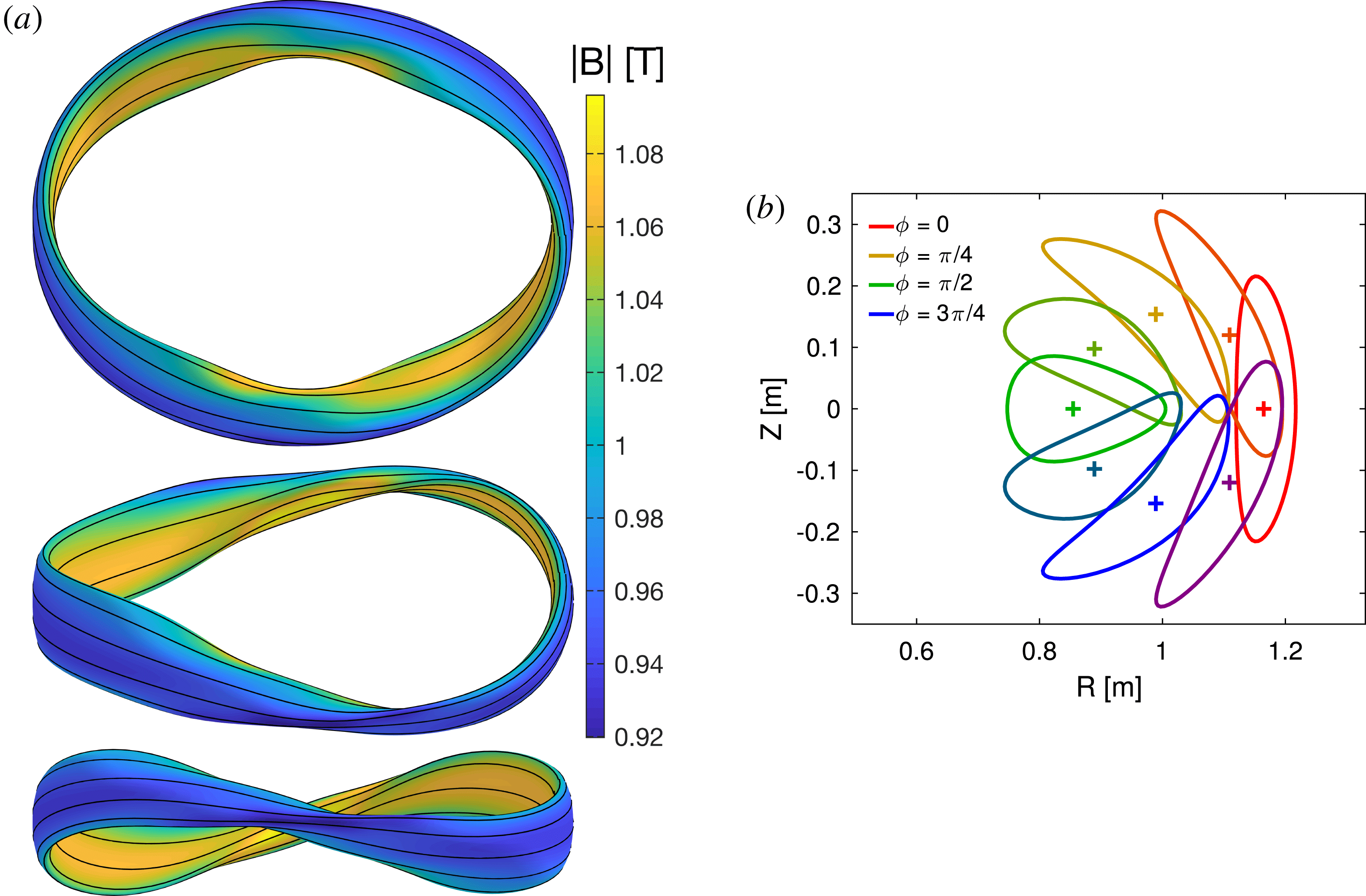
Figure 1. The partially quasi-axisymmetric example of § 5.1, for aspect ratio
 $A=10$
,
$A=10$
,
 $A_{vmec}=9.75$
. The 3-D surface shape in (a), shown from three angles, and the cross-sections in (b), are generated by the construction. In (a), magnetic field lines are shown as black lines, and colour indicates the field strength computed by VMEC.
$A_{vmec}=9.75$
. The 3-D surface shape in (a), shown from three angles, and the cross-sections in (b), are generated by the construction. In (a), magnetic field lines are shown as black lines, and colour indicates the field strength computed by VMEC.
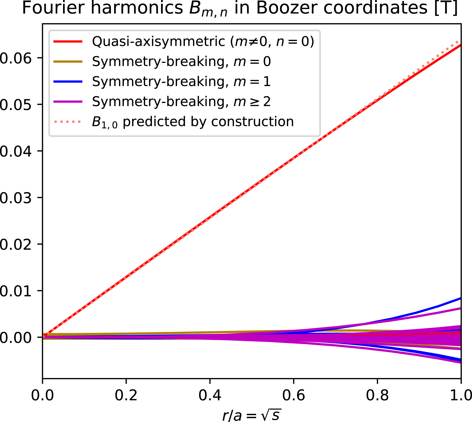
Figure 2. The spectrum of
 $B$
for the partially quasi-axisymmetric example of § 5.1, computed by running the VMEC and BOOZ_XFORM codes inside the constructed boundary surface for aspect ratio
$B$
for the partially quasi-axisymmetric example of § 5.1, computed by running the VMEC and BOOZ_XFORM codes inside the constructed boundary surface for aspect ratio
 $A=10$
,
$A=10$
,
 $A_{vmec}=9.75$
.
$A_{vmec}=9.75$
.
Keeping all input parameters fixed except for the boundary aspect ratio, we then construct boundary surfaces at a sequence of increasing aspect ratios, and repeat the VMEC and BOOZ_XFORM calculations for each case. In figure 3, the quantity
 $[B_{m=0}(\unicode[STIX]{x1D711},r=a)-B(\unicode[STIX]{x1D711},r=0)]/a^{2}$
is displayed for this sequence of numerical calculations. According to the construction, this quantity should be
$[B_{m=0}(\unicode[STIX]{x1D711},r=a)-B(\unicode[STIX]{x1D711},r=0)]/a^{2}$
is displayed for this sequence of numerical calculations. According to the construction, this quantity should be
 $B_{20}(\unicode[STIX]{x1D711})$
. Indeed, it can be seen that the VMEC/BOOZ_XFORM results converge to the Garren–Boozer prediction. Thus, in the limit
$B_{20}(\unicode[STIX]{x1D711})$
. Indeed, it can be seen that the VMEC/BOOZ_XFORM results converge to the Garren–Boozer prediction. Thus, in the limit
 $A\gg 1$
, the full 3-D equilibrium calculations achieve the expected field strength in Boozer coordinates.
$A\gg 1$
, the full 3-D equilibrium calculations achieve the expected field strength in Boozer coordinates.
As another verification of the construction, figure 4 displays three symmetry-breaking measures
 $$\begin{eqnarray}\left.\begin{array}{@{}c@{}}\displaystyle S_{m>0}^{r=a}=\frac{1}{B_{0,0}}\sqrt{\mathop{\sum }_{m>0,n\neq Nm}B_{m,n}^{2}(r=a)},\quad S_{m=0}^{r=a}=\frac{1}{B_{0,0}}\sqrt{\mathop{\sum }_{n\neq 0}B_{0,n}^{2}(r=a)},\\ \displaystyle S_{m=0}^{r=0}=\frac{1}{B_{0,0}}\sqrt{\mathop{\sum }_{n\neq 0}B_{0,n}^{2}(r=0)},\end{array}\right\}\end{eqnarray}$$
computed from the VMEC and BOOZ_XFORM results for the aspect ratio scan. (‘Config 1’ in the figure refers to the present section, while ‘Config 2’ will be described in § 5.2.) It can be seen that
 $S_{m>0}^{r=a}$
scales as
$S_{m>0}^{r=a}$
scales as
 $1/A^{3}$
, consistent with the fact that the corresponding modes were constructed to be zero through
$1/A^{3}$
, consistent with the fact that the corresponding modes were constructed to be zero through
 $O((r/{\mathcal{R}})^{2})$
, so symmetry breaking generally arises at next order. The on-axis mirror modes, measured by
$O((r/{\mathcal{R}})^{2})$
, so symmetry breaking generally arises at next order. The on-axis mirror modes, measured by
 $S_{m=0}^{r=0}$
, are found to have an even stronger scaling,
$S_{m=0}^{r=0}$
, are found to have an even stronger scaling,
 $\propto 1/A^{4}$
. This scaling arises because the
$\propto 1/A^{4}$
. This scaling arises because the
 $m=0$
modes were constructed to be zero through
$m=0$
modes were constructed to be zero through
 $O((r/{\mathcal{R}})^{2})$
, and they are automatically zero at
$O((r/{\mathcal{R}})^{2})$
, and they are automatically zero at
 $O((r/{\mathcal{R}})^{3})$
(only
$O((r/{\mathcal{R}})^{3})$
(only
 $m=1$
and
$m=1$
and
 $m=3$
modes exist at this order), so the first non-vanishing contribution occurs at
$m=3$
modes exist at this order), so the first non-vanishing contribution occurs at
 $O((r/{\mathcal{R}})^{4})$
. Finally,
$O((r/{\mathcal{R}})^{4})$
. Finally,
 $S_{m=0}^{r=a}$
shows an asymptotic scaling
$S_{m=0}^{r=a}$
shows an asymptotic scaling
 $\propto 1/A^{2}$
, associated with the fact that
$\propto 1/A^{2}$
, associated with the fact that
 $B_{20}$
is not independent of
$B_{20}$
is not independent of
 $\unicode[STIX]{x1D711}$
. Thus, all three symmetry-breaking measures scale as predicted by the construction.
$\unicode[STIX]{x1D711}$
. Thus, all three symmetry-breaking measures scale as predicted by the construction.

Figure 3. As the aspect ratio
 $A$
increases, the
$A$
increases, the
 $B_{20}(\unicode[STIX]{x1D711})$
component of the field strength of the numerical VMEC configurations converges to the function predicted by the Garren–Boozer construction. Data here are for the partially quasi-axisymmetric configuration of § 5.1.
$B_{20}(\unicode[STIX]{x1D711})$
component of the field strength of the numerical VMEC configurations converges to the function predicted by the Garren–Boozer construction. Data here are for the partially quasi-axisymmetric configuration of § 5.1.

Figure 4. The measures of quasisymmetry breaking (5.2), computed by running the VMEC and BOOZ_XFORM codes inside the constructed boundary surfaces, scale as the expected power of aspect ratio. Data here are for the partially quasi-axisymmetric and optimized quasi-axisymmetric examples of §§ 5.1 (‘Config 1’) and 5.2 (‘Config 2’).
5.2 Quasi-axisymmetry fully through
$O((r/{\mathcal{R}})^{2})$

We next consider a configuration that is similar to the one of § 5.1, but with slightly different parameters such that
 $B_{20}$
has significantly reduced toroidal variation, resulting in improved quasi-axisymmetry. We again consider a two-field-period device, with axis shape
$B_{20}$
has significantly reduced toroidal variation, resulting in improved quasi-axisymmetry. We again consider a two-field-period device, with axis shape
 $$\begin{eqnarray}\left.\begin{array}{@{}c@{}}R_{0}(\unicode[STIX]{x1D719})~(\text{m})=1+0.173\cos (2\unicode[STIX]{x1D719})+0.0168\cos (4\unicode[STIX]{x1D719})+0.00101\cos (6\unicode[STIX]{x1D719}),\\ z_{0}(\unicode[STIX]{x1D719})~(\text{m})=0.159\sin (2\unicode[STIX]{x1D719})+0.0165\sin (4\unicode[STIX]{x1D719})+0.000985\sin (6\unicode[STIX]{x1D719}).\end{array}\right\}\end{eqnarray}$$
The other non-zero input parameters are
 $\bar{\unicode[STIX]{x1D702}}=0.632~\text{m}^{-1}$
and
$\bar{\unicode[STIX]{x1D702}}=0.632~\text{m}^{-1}$
and
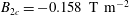 $B_{2c}=-0.158~\text{T}~\text{m}^{-2}$
. These values and axis shape were obtained by the optimization procedure of § 4.3, again minimizing
$B_{2c}=-0.158~\text{T}~\text{m}^{-2}$
. These values and axis shape were obtained by the optimization procedure of § 4.3, again minimizing
 $X_{2}$
,
$X_{2}$
,
 $Y_{2}$
,
$Y_{2}$
,
 $X_{3}$
and
$X_{3}$
and
 $Y_{3}$
, but now also minimizing the toroidal variation of
$Y_{3}$
, but now also minimizing the toroidal variation of
 $B_{20}$
. The parameters
$B_{20}$
. The parameters
 $\unicode[STIX]{x1D70E}(0)$
and
$\unicode[STIX]{x1D70E}(0)$
and
 $B_{2s}$
were again set to zero so the configuration is stellarator symmetric, and
$B_{2s}$
were again set to zero so the configuration is stellarator symmetric, and
 $I_{2}$
and
$I_{2}$
and
 $p_{2}$
were set to zero so the configuration is a vacuum field. The resulting configuration has
$p_{2}$
were set to zero so the configuration is a vacuum field. The resulting configuration has
 $\unicode[STIX]{x1D704}_{0}=0.424$
. The function
$\unicode[STIX]{x1D704}_{0}=0.424$
. The function
 $B_{20}(\unicode[STIX]{x1D711})$
for these parameters is shown as the black dotted curve in figure 7, and it can be seen that the toroidal variation is greatly reduced compared to figure 3. The small remaining toroidal variation of
$B_{20}(\unicode[STIX]{x1D711})$
for these parameters is shown as the black dotted curve in figure 7, and it can be seen that the toroidal variation is greatly reduced compared to figure 3. The small remaining toroidal variation of
 $B_{20}$
could presumably be further reduced if additional Fourier modes were included in the axis shape. The constructed boundary shape for
$B_{20}$
could presumably be further reduced if additional Fourier modes were included in the axis shape. The constructed boundary shape for
 $A=10$
is shown in figure 5, and it is only slightly different from the previous example (figure 1.) Running VMEC and BOOZ_XFORM inside this boundary results in the magnetic spectrum of figure 6. Again, the desired mode
$A=10$
is shown in figure 5, and it is only slightly different from the previous example (figure 1.) Running VMEC and BOOZ_XFORM inside this boundary results in the magnetic spectrum of figure 6. Again, the desired mode
 $B_{1,0}$
dominates, and its magnitude is nearly identical to the prediction. Figure 7 shows that
$B_{1,0}$
dominates, and its magnitude is nearly identical to the prediction. Figure 7 shows that
 $[B_{m=0}(\unicode[STIX]{x1D711},r=a)-B(\unicode[STIX]{x1D711},r=0)]/a^{2}$
again converges to the predicted function,
$[B_{m=0}(\unicode[STIX]{x1D711},r=a)-B(\unicode[STIX]{x1D711},r=0)]/a^{2}$
again converges to the predicted function,
 $B_{20}(\unicode[STIX]{x1D711})$
.
$B_{20}(\unicode[STIX]{x1D711})$
.
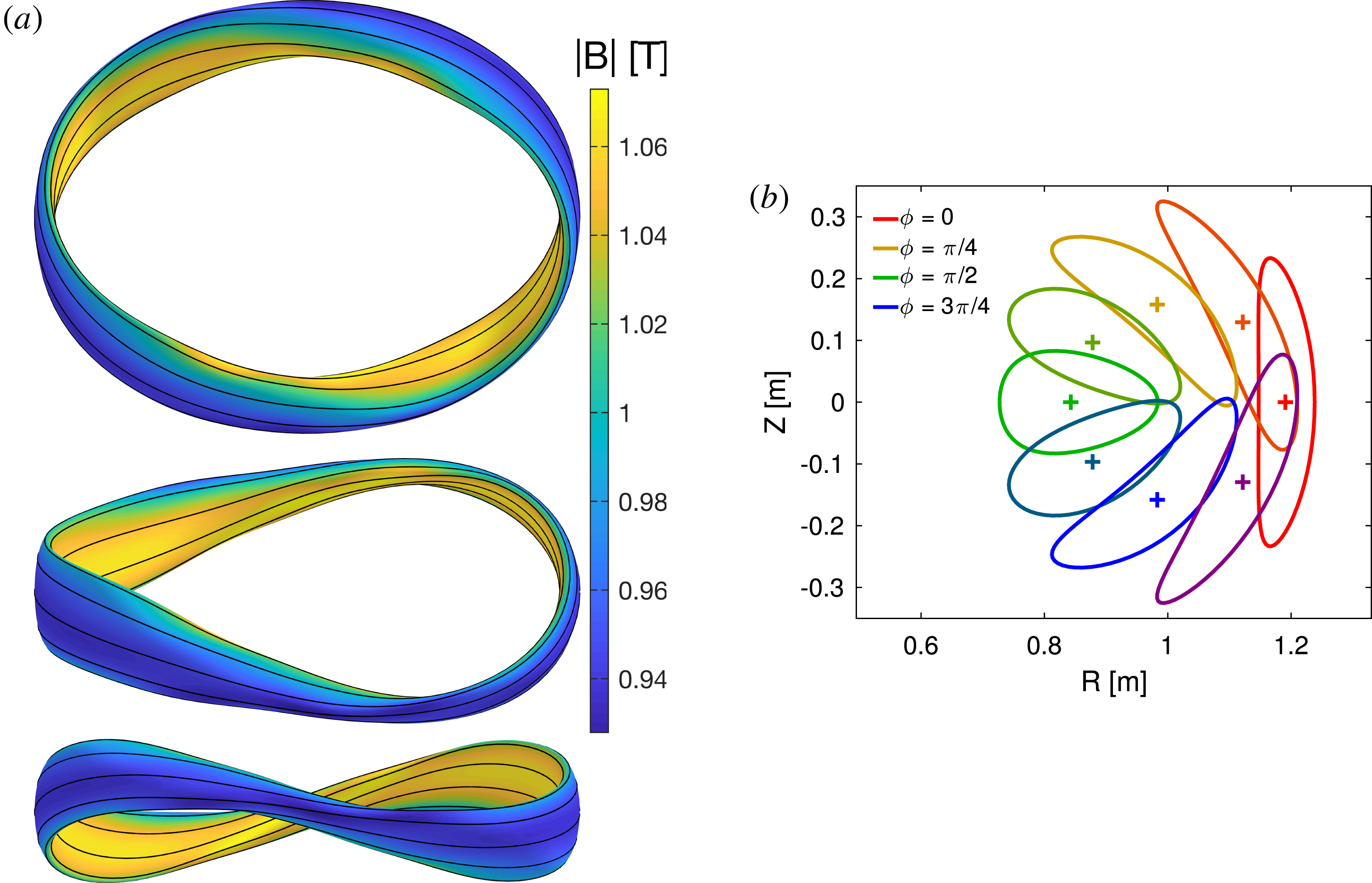
Figure 5. The quasi-axisymmetric example of § 5.2, for aspect ratio
 $A=10$
,
$A=10$
,
 $A_{vmec}=9.71$
. The 3-D surface shape in (a), shown from three angles, and the cross-sections in (b), are generated by the construction. In (a), magnetic field lines are shown as black lines, and colour indicates the field strength computed by VMEC.
$A_{vmec}=9.71$
. The 3-D surface shape in (a), shown from three angles, and the cross-sections in (b), are generated by the construction. In (a), magnetic field lines are shown as black lines, and colour indicates the field strength computed by VMEC.

Figure 6. The spectrum of
 $B$
for the quasi-axisymmetric example of § 5.2, computed by running the VMEC and BOOZ_XFORM codes inside the constructed boundary surface for aspect ratio
$B$
for the quasi-axisymmetric example of § 5.2, computed by running the VMEC and BOOZ_XFORM codes inside the constructed boundary surface for aspect ratio
 $A=10$
,
$A=10$
,
 $A_{vmec}=9.71$
.
$A_{vmec}=9.71$
.
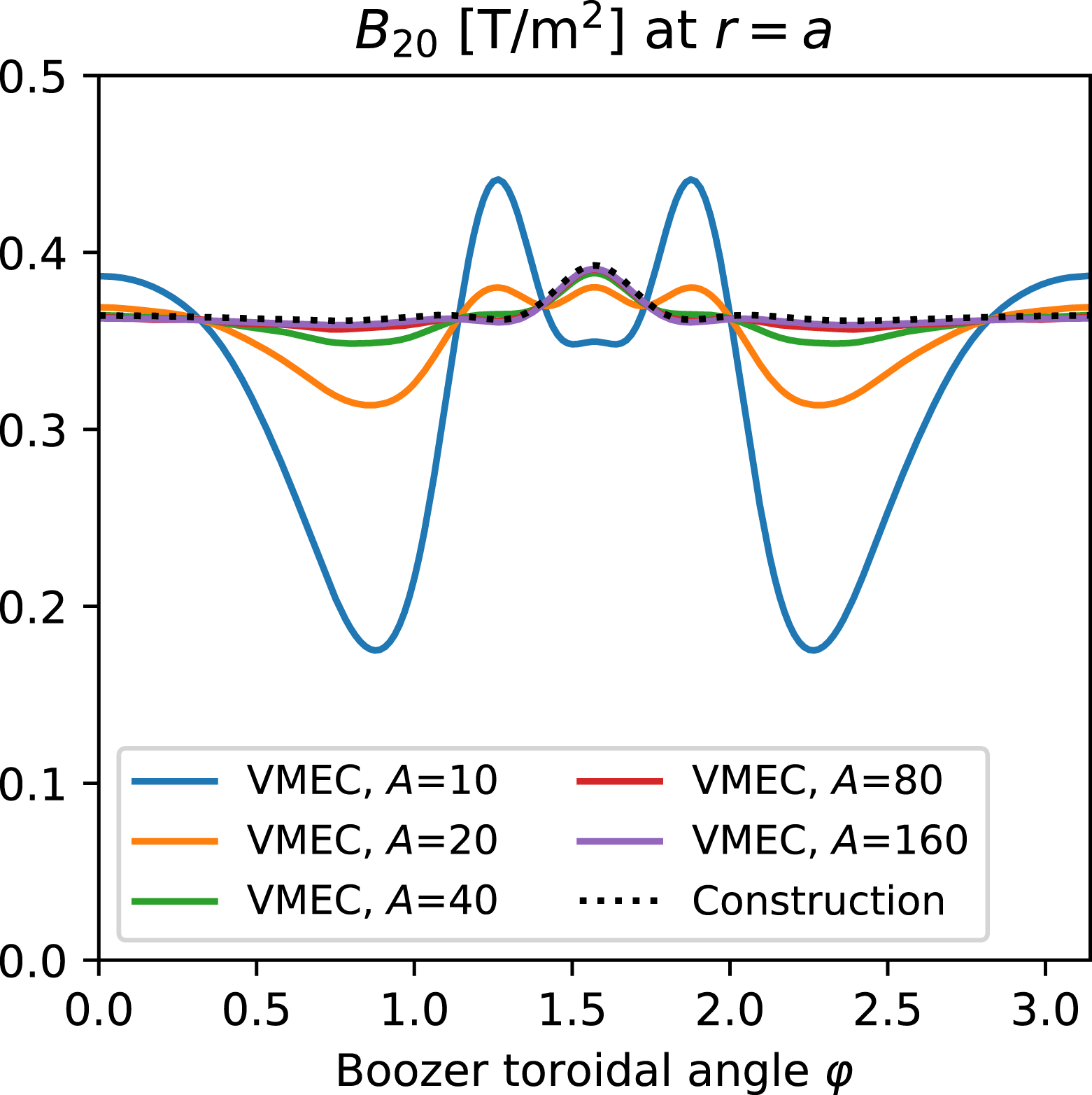
Figure 7. As the aspect ratio
 $A$
increases, the
$A$
increases, the
 $B_{20}(\unicode[STIX]{x1D711})$
component of the field strength of the numerical VMEC configurations converges to the function predicted by the Garren–Boozer construction. Data here are for the quasi-axisymmetric configuration of § 5.2.
$B_{20}(\unicode[STIX]{x1D711})$
component of the field strength of the numerical VMEC configurations converges to the function predicted by the Garren–Boozer construction. Data here are for the quasi-axisymmetric configuration of § 5.2.
The three symmetry-breaking measures for this second configuration are displayed in figure 4, labelled as ‘Config 2’. It can be seen that
 $S_{m>0}^{r=a}$
and
$S_{m>0}^{r=a}$
and
 $S_{m=0}^{r=0}$
are not much changed from the first configuration, scaling as
$S_{m=0}^{r=0}$
are not much changed from the first configuration, scaling as
 $1/A^{3}$
and
$1/A^{3}$
and
 $1/A^{4}$
, as before. However,
$1/A^{4}$
, as before. However,
 $S_{m=0}^{r=a}$
is significantly changed, still scaling as
$S_{m=0}^{r=a}$
is significantly changed, still scaling as
 $1/A^{2}$
for sufficiently large
$1/A^{2}$
for sufficiently large
 $A$
, but with the leading constant reduced by over an order of magnitude. This reduction reflects the reduced variation of
$A$
, but with the leading constant reduced by over an order of magnitude. This reduction reflects the reduced variation of
 $B_{20}$
. For
$B_{20}$
. For
 $A<40$
,
$A<40$
,
 $S_{m=0}^{r=a}$
now scales as
$S_{m=0}^{r=a}$
now scales as
 $1/A^{4}$
since it is dominated by the on-axis variation of
$1/A^{4}$
since it is dominated by the on-axis variation of
 $B$
measured by
$B$
measured by
 $S_{m=0}^{r=0}$
. Thus,
$S_{m=0}^{r=0}$
. Thus,
 $B_{20}$
is constant enough that it is not the dominant source of symmetry breaking for the entire range of aspect ratios shown,
$B_{20}$
is constant enough that it is not the dominant source of symmetry breaking for the entire range of aspect ratios shown,
 $A\in [5,320]$
. This point is apparent also in figure 8, in which the quantity plotted
$A\in [5,320]$
. This point is apparent also in figure 8, in which the quantity plotted
 $$\begin{eqnarray}S_{\text{tot}}=\frac{1}{B_{0,0}}\sqrt{\mathop{\sum }_{m,n\neq Nm}B_{m,n}^{2}(r=a)}\end{eqnarray}$$
includes all quasisymmetry-breaking modes. This figure more clearly shows the scaling predicted by Garren & Boozer (Reference Garren and Boozer1991a
) that the total deviation from quasisymmetry can be made to scale as
 $\propto 1/A^{3}$
. The quasisymmetry of this quasi-axisymmetric configuration is sufficiently good that, for
$\propto 1/A^{3}$
. The quasisymmetry of this quasi-axisymmetric configuration is sufficiently good that, for
 $A\geqslant 60$
, the deviation from quasisymmetry
$A\geqslant 60$
, the deviation from quasisymmetry
 $S_{\text{tot}}B_{0}$
is smaller than the Earth’s magnetic field of
$S_{\text{tot}}B_{0}$
is smaller than the Earth’s magnetic field of
 ${\sim}0.5$
Gauss. At the right-most point (
${\sim}0.5$
Gauss. At the right-most point (
 $A=320$
),
$A=320$
),
 $S_{\text{tot}}$
is
$S_{\text{tot}}$
is
 ${<}4\times 10^{-7}$
, and the largest single symmetry-breaking Fourier mode has an amplitude
${<}4\times 10^{-7}$
, and the largest single symmetry-breaking Fourier mode has an amplitude
 ${<}2\times 10^{-7}~\text{T}$
.
${<}2\times 10^{-7}~\text{T}$
.
Figure 8. A numerical demonstration of the prediction by Garren & Boozer (Reference Garren and Boozer1991a
) that deviations from quasisymmetry can be made to scale as
 $1/A^{3}$
. Here, the deviations are measured by (5.4) for the configurations of §§ 5.2 and 5.4.
$1/A^{3}$
. Here, the deviations are measured by (5.4) for the configurations of §§ 5.2 and 5.4.
5.3 Tokamak–stellarator hybrid
To verify the construction for a case in which the plasma pressure and on-axis current are non-zero, we next consider a tokamak–stellarator hybrid configuration, in which both non-axisymmetric shaping and toroidal current contribute to the rotational transform. We again consider a two-field-period geometry, with axis shape
 $$\begin{eqnarray}\left.\begin{array}{@{}c@{}}R_{0}(\unicode[STIX]{x1D719})~(\text{m})=1+0.09\cos (2\unicode[STIX]{x1D719}),\\ z_{0}(\unicode[STIX]{x1D719})~(\text{m})=-0.09\sin (2\unicode[STIX]{x1D719}).\end{array}\right\}\end{eqnarray}$$
The parameters
 $\unicode[STIX]{x1D70E}(0)$
and
$\unicode[STIX]{x1D70E}(0)$
and
 $B_{2s}$
were again set to zero so the configuration is stellarator symmetric. The other input parameters were
$B_{2s}$
were again set to zero so the configuration is stellarator symmetric. The other input parameters were
 $\bar{\unicode[STIX]{x1D702}}=0.95~\text{m}^{-1}$
,
$\bar{\unicode[STIX]{x1D702}}=0.95~\text{m}^{-1}$
,
 $I_{2}=0.9~\text{T}~\text{m}^{-1}$
,
$I_{2}=0.9~\text{T}~\text{m}^{-1}$
,
 $p_{2}=-6\times 10^{5}~\text{Pa}~\text{m}^{-2}$
and
$p_{2}=-6\times 10^{5}~\text{Pa}~\text{m}^{-2}$
and
 $B_{2c}=-0.7~\text{T}~\text{m}^{-2}$
. For this value of
$B_{2c}=-0.7~\text{T}~\text{m}^{-2}$
. For this value of
 $p_{2}$
, the volume-averaged
$p_{2}$
, the volume-averaged
 $\unicode[STIX]{x1D6FD}$
(plasma pressure/magnetic pressure) for the configuration at
$\unicode[STIX]{x1D6FD}$
(plasma pressure/magnetic pressure) for the configuration at
 $A=5$
is 2.9 %. The resulting configuration has
$A=5$
is 2.9 %. The resulting configuration has
 $\unicode[STIX]{x1D704}_{0}=0.960$
. For comparison, a vacuum field inside the constructed
$\unicode[STIX]{x1D704}_{0}=0.960$
. For comparison, a vacuum field inside the constructed
 $A=5$
boundary has an on-axis transform
$A=5$
boundary has an on-axis transform
 $\unicode[STIX]{x1D704}_{0}=0.214$
. This level of vacuum transform might be sufficient to provide stellarator-like stability. The boundary shape for
$\unicode[STIX]{x1D704}_{0}=0.214$
. This level of vacuum transform might be sufficient to provide stellarator-like stability. The boundary shape for
 $A=5$
is shown in figure 9. Figure 10 shows the Boozer spectrum of the finite-
$A=5$
is shown in figure 9. Figure 10 shows the Boozer spectrum of the finite-
 $\unicode[STIX]{x1D6FD}$
finite-current configuration inside this boundary. While the desired mode
$\unicode[STIX]{x1D6FD}$
finite-current configuration inside this boundary. While the desired mode
 $B_{1,0}$
dominates, and it has a magnitude close to that predicted by the construction, the departures from quasisymmetry are larger than in the previous examples, associated with the smaller value of
$B_{1,0}$
dominates, and it has a magnitude close to that predicted by the construction, the departures from quasisymmetry are larger than in the previous examples, associated with the smaller value of
 $A$
here. Figure 11 shows that as
$A$
here. Figure 11 shows that as
 $A$
is increased,
$A$
is increased,
 $[B_{m=0}(\unicode[STIX]{x1D711},r=a)-B(\unicode[STIX]{x1D711},r=0)]/a^{2}$
again converges to the predicted function,
$[B_{m=0}(\unicode[STIX]{x1D711},r=a)-B(\unicode[STIX]{x1D711},r=0)]/a^{2}$
again converges to the predicted function,
 $B_{20}(\unicode[STIX]{x1D711})$
. The scaling of the three symmetry-breaking measures with
$B_{20}(\unicode[STIX]{x1D711})$
. The scaling of the three symmetry-breaking measures with
 $A$
is plotted in figure 12, and again, they scale as the expected power of
$A$
is plotted in figure 12, and again, they scale as the expected power of
 $A$
. Together, figures 11–12 verify the
$A$
. Together, figures 11–12 verify the
 $O((r/{\mathcal{R}})^{2})$
construction behaves correctly when
$O((r/{\mathcal{R}})^{2})$
construction behaves correctly when
 $I_{2}$
and
$I_{2}$
and
 $p_{2}$
terms are included.
$p_{2}$
terms are included.
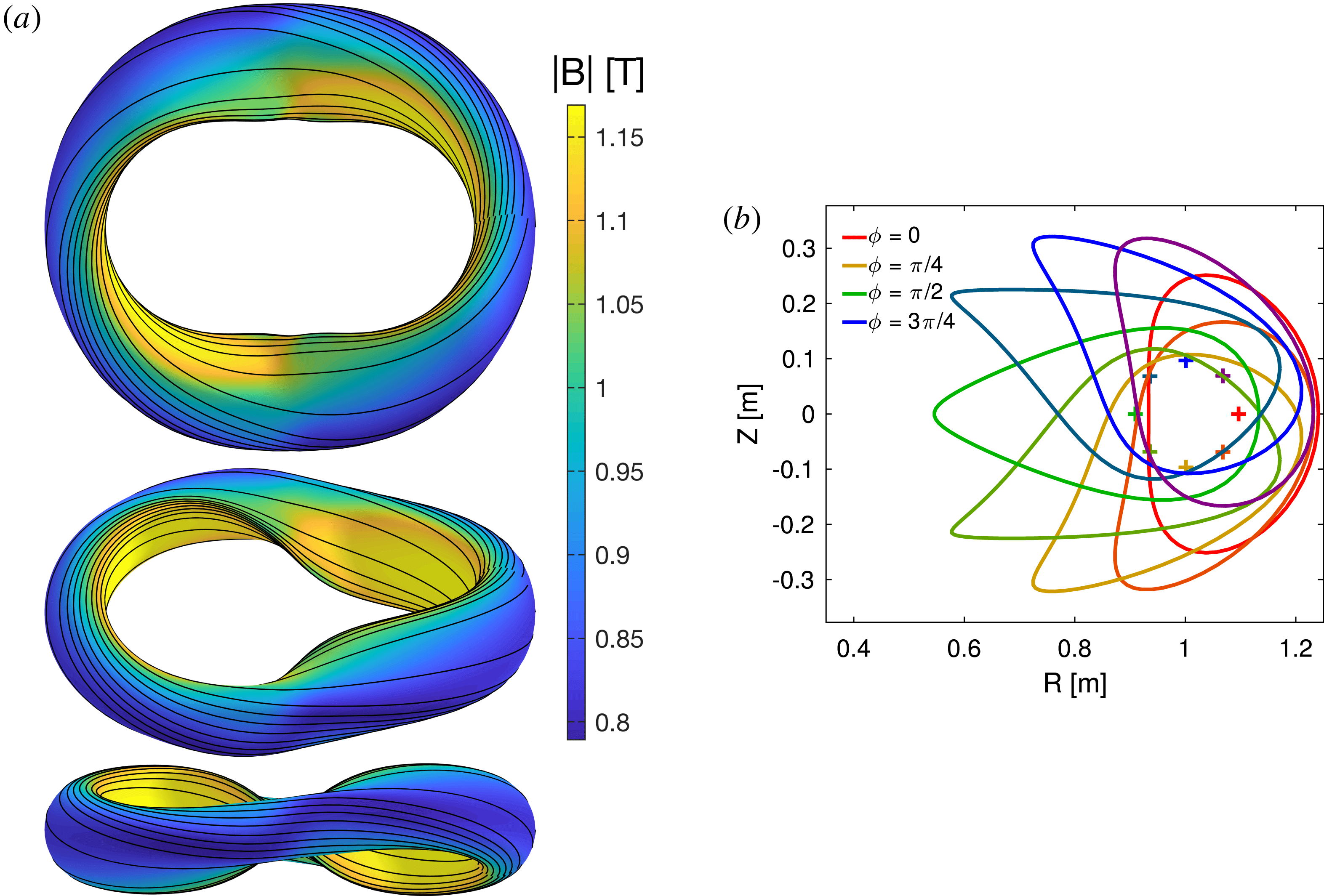
Figure 9. The tokamak–stellarator hybrid example of § 5.3, for aspect ratio
 $A=5$
,
$A=5$
,
 $A_{vmec}=4.87$
. The 3-D surface shape in (a), shown from three angles, and the cross-sections in (b), are generated by the construction. In (a), magnetic field lines are shown as black lines, and colour indicates the field strength computed by VMEC.
$A_{vmec}=4.87$
. The 3-D surface shape in (a), shown from three angles, and the cross-sections in (b), are generated by the construction. In (a), magnetic field lines are shown as black lines, and colour indicates the field strength computed by VMEC.
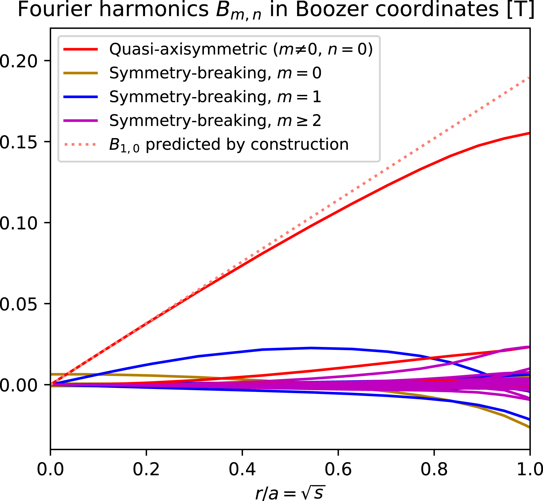
Figure 10. The spectrum of
 $B$
for the tokamak–stellarator hybrid example of § 5.3, computed by running the VMEC and BOOZ_XFORM codes inside the constructed boundary surface for aspect ratio
$B$
for the tokamak–stellarator hybrid example of § 5.3, computed by running the VMEC and BOOZ_XFORM codes inside the constructed boundary surface for aspect ratio
 $A=5$
,
$A=5$
,
 $A_{vmec}=4.87$
.
$A_{vmec}=4.87$
.

Figure 11. As the aspect ratio
 $A$
increases, the
$A$
increases, the
 $B_{20}(\unicode[STIX]{x1D711})$
component of the field strength of the numerical VMEC configurations converges to the function predicted by the Garren–Boozer construction. Data here are for the tokamak–stellarator hybrid configuration of § 5.3.
$B_{20}(\unicode[STIX]{x1D711})$
component of the field strength of the numerical VMEC configurations converges to the function predicted by the Garren–Boozer construction. Data here are for the tokamak–stellarator hybrid configuration of § 5.3.

5.4 Quasi-helical symmetry
We next consider a quasi-helically symmetric configuration. The axis shape is taken to be
 $$\begin{eqnarray}\left.\begin{array}{@{}c@{}}\begin{array}{@{}rcl@{}}R_{0}(\unicode[STIX]{x1D719})~(\text{m})\; & =\; & 1+0.1700\cos (4\unicode[STIX]{x1D719})+0.01804\cos (8\unicode[STIX]{x1D719})+0.001409\cos (12\unicode[STIX]{x1D719})\\ \; & \; & +\,0.00005877\cos (16\unicode[STIX]{x1D719}),\end{array}\\ \begin{array}{@{}rcl@{}}z_{0}(\unicode[STIX]{x1D719})~(\text{m})\; & =\; & 0.1583\sin (4\unicode[STIX]{x1D719})+0.01820\sin (8\unicode[STIX]{x1D719})+0.001548\sin (12\unicode[STIX]{x1D719})\\ \; & \; & +\,0.00007772\sin (16\unicode[STIX]{x1D719}),\end{array}\end{array}\right\}\end{eqnarray}$$
with
 $\bar{\unicode[STIX]{x1D702}}=1.569~\text{m}^{-1}$
and
$\bar{\unicode[STIX]{x1D702}}=1.569~\text{m}^{-1}$
and
 $B_{2c}=0.1348~\text{T}~\text{m}^{-2}$
. These values were obtained using the optimization procedure of § 4.3 to minimize
$B_{2c}=0.1348~\text{T}~\text{m}^{-2}$
. These values were obtained using the optimization procedure of § 4.3 to minimize
 $X_{2}$
,
$X_{2}$
,
 $Y_{2}$
,
$Y_{2}$
,
 $X_{3}$
and
$X_{3}$
and
 $Y_{3}$
. For this axis shape, the normal vector rotates around the axis poloidally four times as the axis is traversed toroidally, so the construction yields quasi-helical symmetry rather than quasi-axisymmetry. The parameters
$Y_{3}$
. For this axis shape, the normal vector rotates around the axis poloidally four times as the axis is traversed toroidally, so the construction yields quasi-helical symmetry rather than quasi-axisymmetry. The parameters
 $\unicode[STIX]{x1D70E}(0)$
and
$\unicode[STIX]{x1D70E}(0)$
and
 $B_{2s}$
were set to zero so the configuration is stellarator symmetric. The other input parameters were
$B_{2s}$
were set to zero so the configuration is stellarator symmetric. The other input parameters were
 $I_{2}=0$
and
$I_{2}=0$
and
 $p_{2}=0$
. The resulting configuration has
$p_{2}=0$
. The resulting configuration has
 $\unicode[STIX]{x1D704}_{0}=1.14$
. The constructed boundary shape for
$\unicode[STIX]{x1D704}_{0}=1.14$
. The constructed boundary shape for
 $A=8$
is shown in figure 13.
$A=8$
is shown in figure 13.

Figure 13. The quasi-helically symmetric example of § 5.4, for aspect ratio
 $A=8$
,
$A=8$
,
 $A_{vmec}=7.14$
. The 3-D surface shape in (a), shown from three angles, and the cross-sections in (b), are generated by the construction. In (a), magnetic field lines are shown as black lines, and colour indicates the field strength computed by VMEC.
$A_{vmec}=7.14$
. The 3-D surface shape in (a), shown from three angles, and the cross-sections in (b), are generated by the construction. In (a), magnetic field lines are shown as black lines, and colour indicates the field strength computed by VMEC.
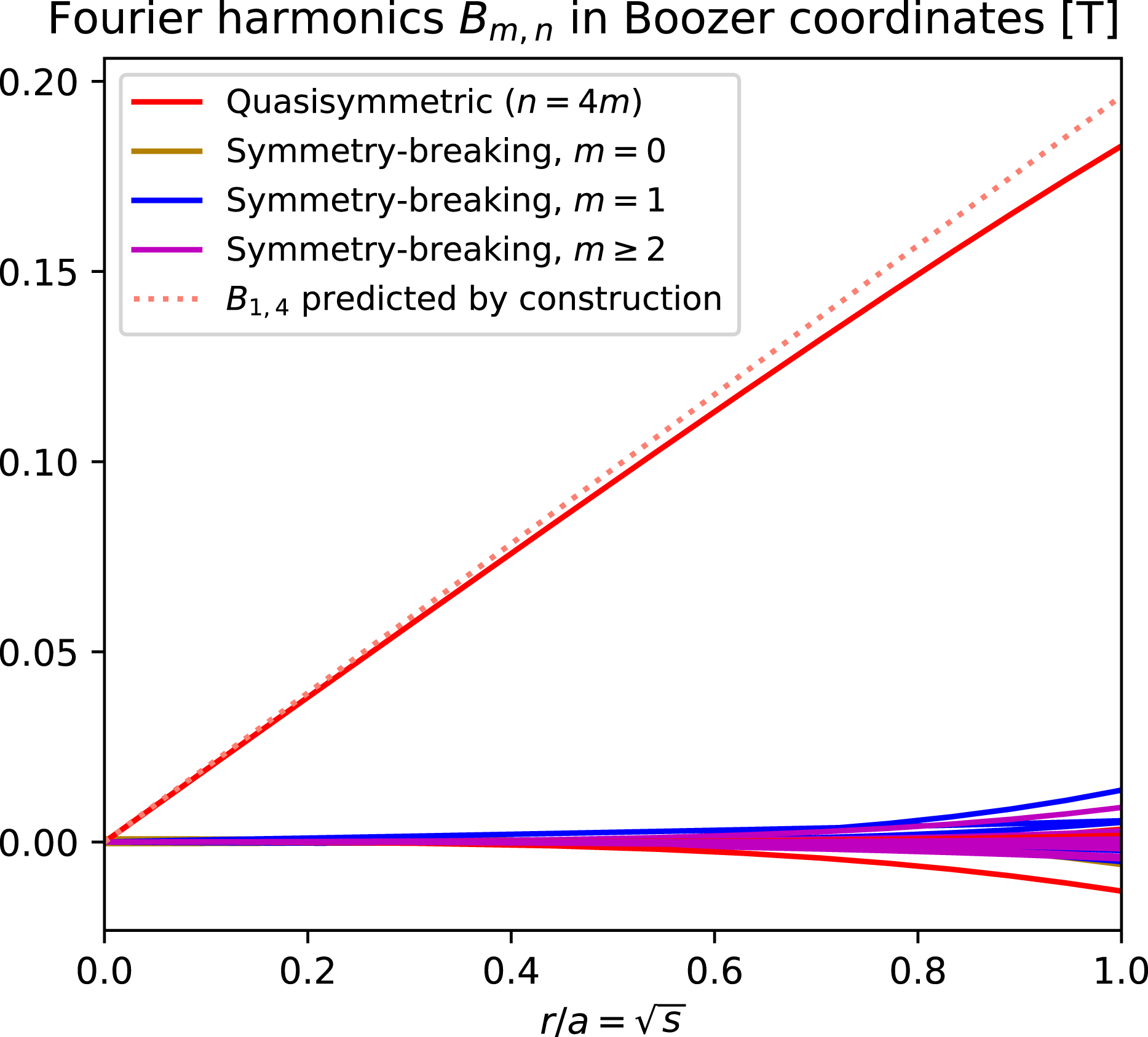
Figure 14. The spectrum of
 $B$
for the quasi-helically symmetric example of § 5.4, computed by running the VMEC and BOOZ_XFORM codes inside the constructed boundary surface for aspect ratio
$B$
for the quasi-helically symmetric example of § 5.4, computed by running the VMEC and BOOZ_XFORM codes inside the constructed boundary surface for aspect ratio
 $A=8$
,
$A=8$
,
 $A_{vmec}=7.14$
.
$A_{vmec}=7.14$
.
Compared to the case of quasi-axisymmetry, for quasi-helical symmetry it seems relatively hard to find sets of input parameters for which
 $X_{2}$
,
$X_{2}$
,
 $Y_{2}$
,
$Y_{2}$
,
 $X_{3}$
and
$X_{3}$
and
 $Y_{3}$
are acceptably small. If these quantities are not small, the boundary aspect ratio must be large, or else the symmetry-breaking errors tend to be large and the boundary surface may self-intersect. This challenge for finding good quasi-helically symmetric configurations likely arises from the fact that they require significant helical excursion of the axis, implying larger
$Y_{3}$
are acceptably small. If these quantities are not small, the boundary aspect ratio must be large, or else the symmetry-breaking errors tend to be large and the boundary surface may self-intersect. This challenge for finding good quasi-helically symmetric configurations likely arises from the fact that they require significant helical excursion of the axis, implying larger
 $\unicode[STIX]{x1D70F}$
and
$\unicode[STIX]{x1D70F}$
and
 $\unicode[STIX]{x1D705}$
compared to quasi-axisymmetric configurations, which act to drive larger
$\unicode[STIX]{x1D705}$
compared to quasi-axisymmetric configurations, which act to drive larger
 $X_{2}$
and
$X_{2}$
and
 $Y_{2}$
. The configuration in this section manages to have small values of
$Y_{2}$
. The configuration in this section manages to have small values of
 $\{X_{2},Y_{2},X_{3},Y_{3}\}$
due to some delicate balances in the equations of appendix A. For instance, merely rounding the coefficients in the axis shape (5.6) to 3 digits of precision rather than 4 causes significant increases in
$\{X_{2},Y_{2},X_{3},Y_{3}\}$
due to some delicate balances in the equations of appendix A. For instance, merely rounding the coefficients in the axis shape (5.6) to 3 digits of precision rather than 4 causes significant increases in
 $X_{3}$
and
$X_{3}$
and
 $Y_{3}$
that result in visible changes to the boundary shape.
$Y_{3}$
that result in visible changes to the boundary shape.
As with the earlier configurations, VMEC and BOOZ_XFORM calculations for this quasi-helically symmetric configuration confirm that the desired field strength is produced. One aspect of this verification is shown in figure 14, which displays the Boozer spectrum inside the constructed
 $A=8$
boundary. This time the dominant mode is
$A=8$
boundary. This time the dominant mode is
 $B_{1,4}$
, and the magnitude of this mode matches the prediction
$B_{1,4}$
, and the magnitude of this mode matches the prediction
 $r\bar{\unicode[STIX]{x1D702}}B_{0}$
. Figure 15 shows that as
$r\bar{\unicode[STIX]{x1D702}}B_{0}$
. Figure 15 shows that as
 $A\rightarrow \infty$
,
$A\rightarrow \infty$
,
 $[B_{m=0}(\unicode[STIX]{x1D711},r=a)-B(\unicode[STIX]{x1D711},r=0)]/a^{2}$
again converges to the predicted function,
$[B_{m=0}(\unicode[STIX]{x1D711},r=a)-B(\unicode[STIX]{x1D711},r=0)]/a^{2}$
again converges to the predicted function,
 $B_{20}(\unicode[STIX]{x1D711})$
. Figure 16 shows that
$B_{20}(\unicode[STIX]{x1D711})$
. Figure 16 shows that
 $S_{m>0}^{r=a}$
,
$S_{m>0}^{r=a}$
,
 $S_{m=0}^{r=a}$
and
$S_{m=0}^{r=a}$
and
 $S_{m=0}^{r=0}$
scale approximately as expected (
$S_{m=0}^{r=0}$
scale approximately as expected (
 $1/A^{3}$
,
$1/A^{3}$
,
 $1/A^{4}$
transitioning to
$1/A^{4}$
transitioning to
 $1/A^{2}$
at large
$1/A^{2}$
at large
 $A$
, and
$A$
, and
 $1/A^{4}$
), as for the previous configurations. The total deviation from quasisymmetry
$1/A^{4}$
), as for the previous configurations. The total deviation from quasisymmetry
 $S_{\text{tot}}$
is also displayed in figure 8, demonstrating again Garren and Boozer’s predicted scaling. (The range of aspect ratios plotted differs from that for the quasi-axisymmetric configuration since at the highest
$S_{\text{tot}}$
is also displayed in figure 8, demonstrating again Garren and Boozer’s predicted scaling. (The range of aspect ratios plotted differs from that for the quasi-axisymmetric configuration since at the highest
 $A$
, it is difficult to obtain converged values from VMEC for the very small symmetry-breaking modes.)
$A$
, it is difficult to obtain converged values from VMEC for the very small symmetry-breaking modes.)
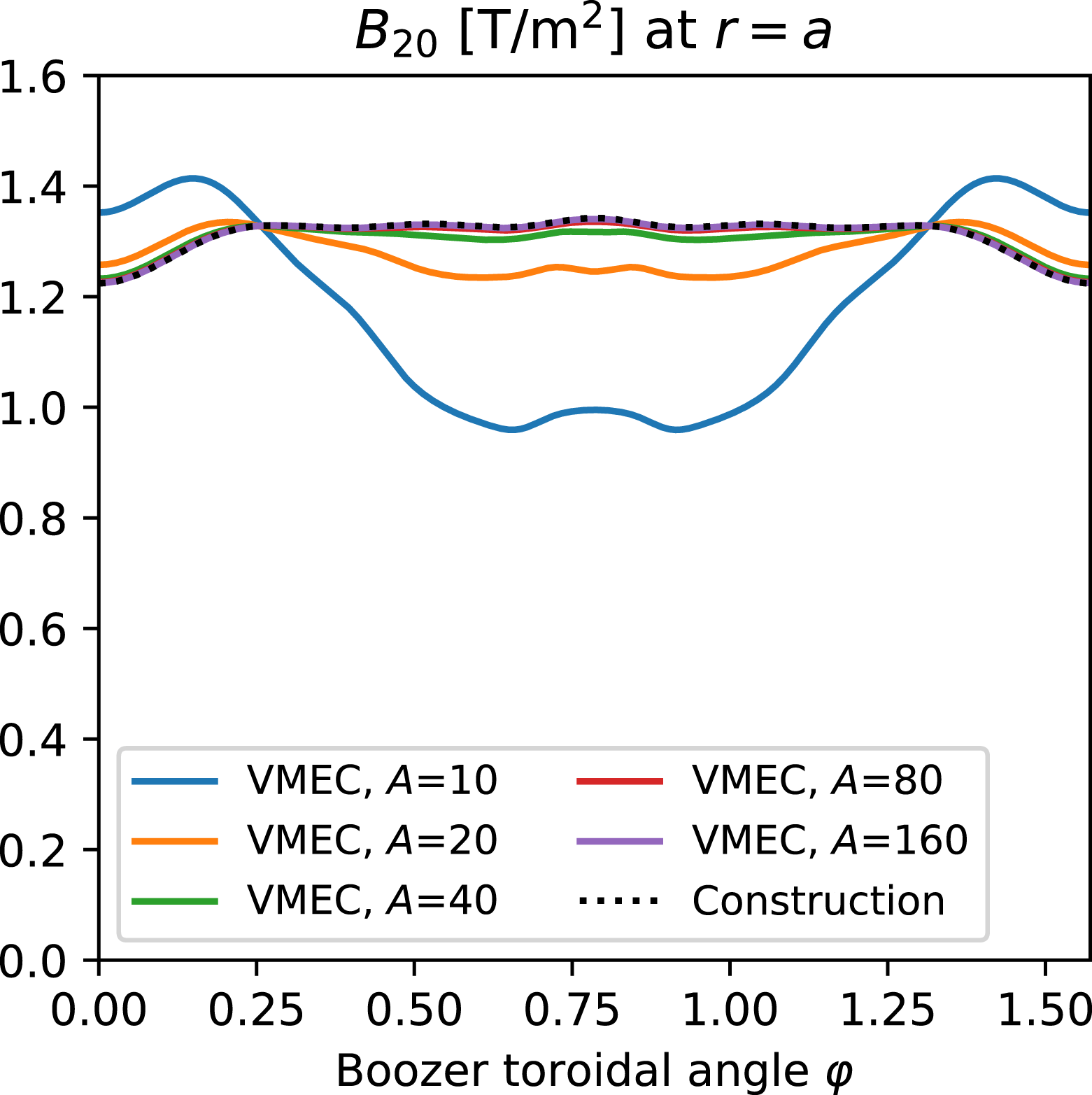
Figure 15. As the aspect ratio
 $A$
increases, the
$A$
increases, the
 $B_{20}(\unicode[STIX]{x1D711})$
component of the field strength of the numerical VMEC configurations converges to the function predicted by the Garren–Boozer construction. Data here are for the quasi-helically symmetric configuration of § 5.4.
$B_{20}(\unicode[STIX]{x1D711})$
component of the field strength of the numerical VMEC configurations converges to the function predicted by the Garren–Boozer construction. Data here are for the quasi-helically symmetric configuration of § 5.4.
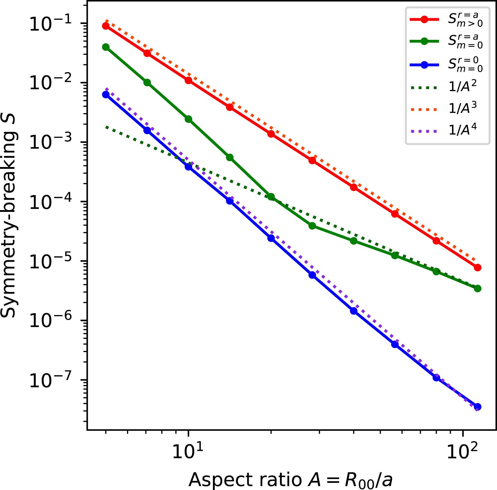
5.5 Testing all terms
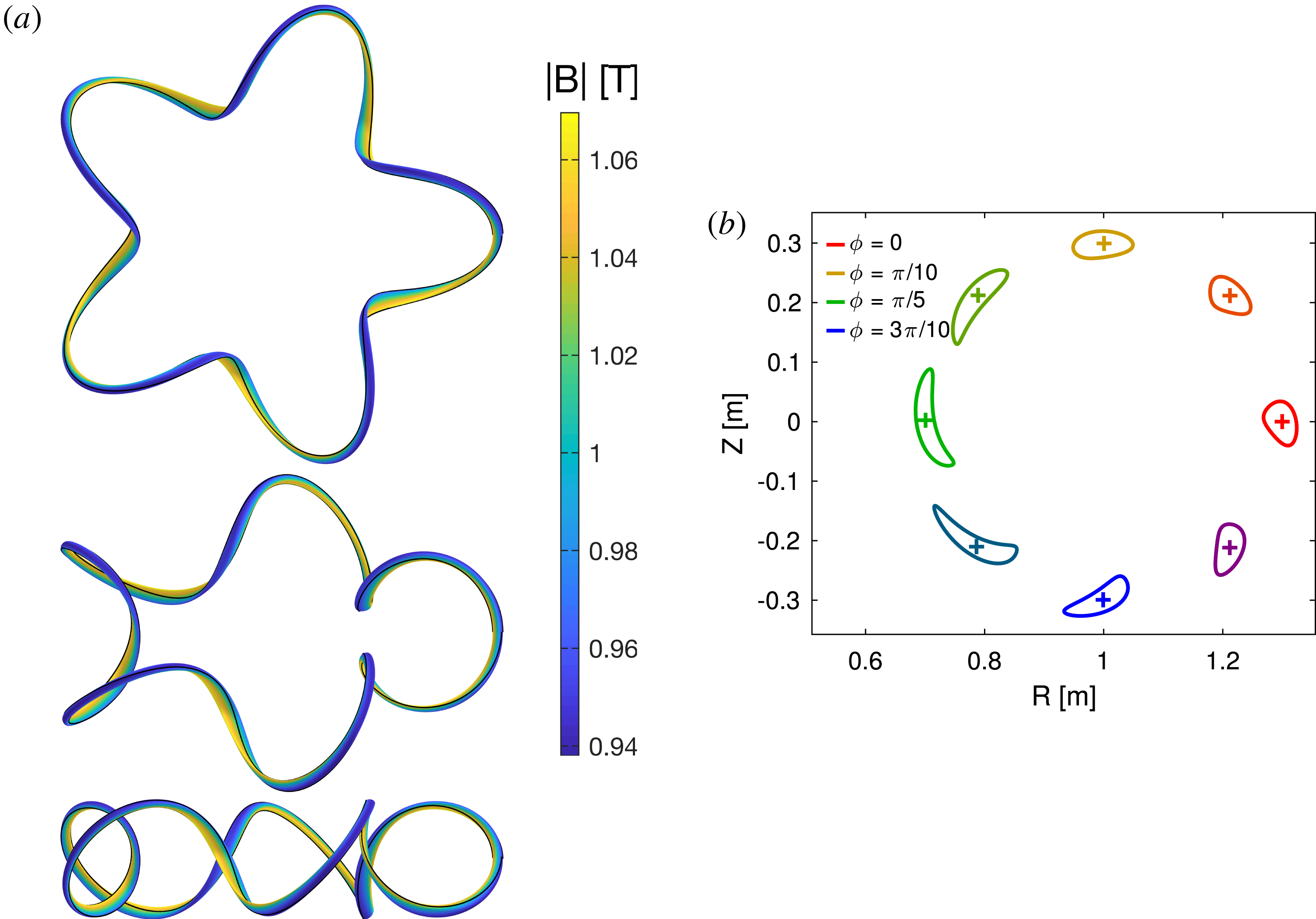
Figure 17. The non-stellarator-symmetric quasi-helically symmetric example of § 5.5, for aspect ratio
 $A=40$
,
$A=40$
,
 $A_{vmec}=28.5$
. The 3-D surface shape in (a), shown from three angles, and the cross-sections in (b), are generated by the construction. In (a), magnetic field lines are shown as black lines, and colour indicates the field strength computed by VMEC.
$A_{vmec}=28.5$
. The 3-D surface shape in (a), shown from three angles, and the cross-sections in (b), are generated by the construction. In (a), magnetic field lines are shown as black lines, and colour indicates the field strength computed by VMEC.
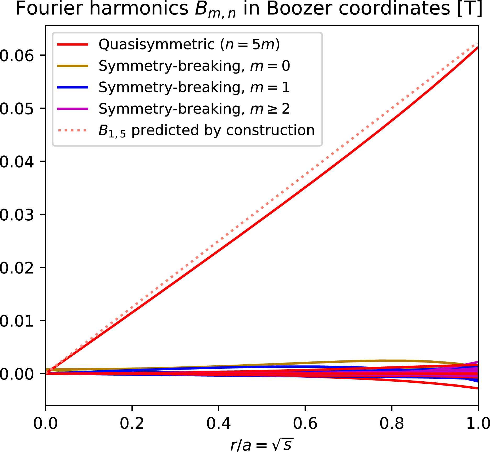
Figure 18. The spectrum of
 $B$
(including both
$B$
(including both
 $\propto \cos (m\unicode[STIX]{x1D703}-n\unicode[STIX]{x1D711})$
and
$\propto \cos (m\unicode[STIX]{x1D703}-n\unicode[STIX]{x1D711})$
and
 $\propto \sin (m\unicode[STIX]{x1D703}-n\unicode[STIX]{x1D711})$
modes) for the non-stellarator-symmetric quasi-helically symmetric example of § 5.5, computed by running the VMEC and BOOZ_XFORM codes inside the constructed boundary surface for aspect ratio
$\propto \sin (m\unicode[STIX]{x1D703}-n\unicode[STIX]{x1D711})$
modes) for the non-stellarator-symmetric quasi-helically symmetric example of § 5.5, computed by running the VMEC and BOOZ_XFORM codes inside the constructed boundary surface for aspect ratio
 $A=40$
,
$A=40$
,
 $A_{vmec}=28.5$
.
$A_{vmec}=28.5$
.
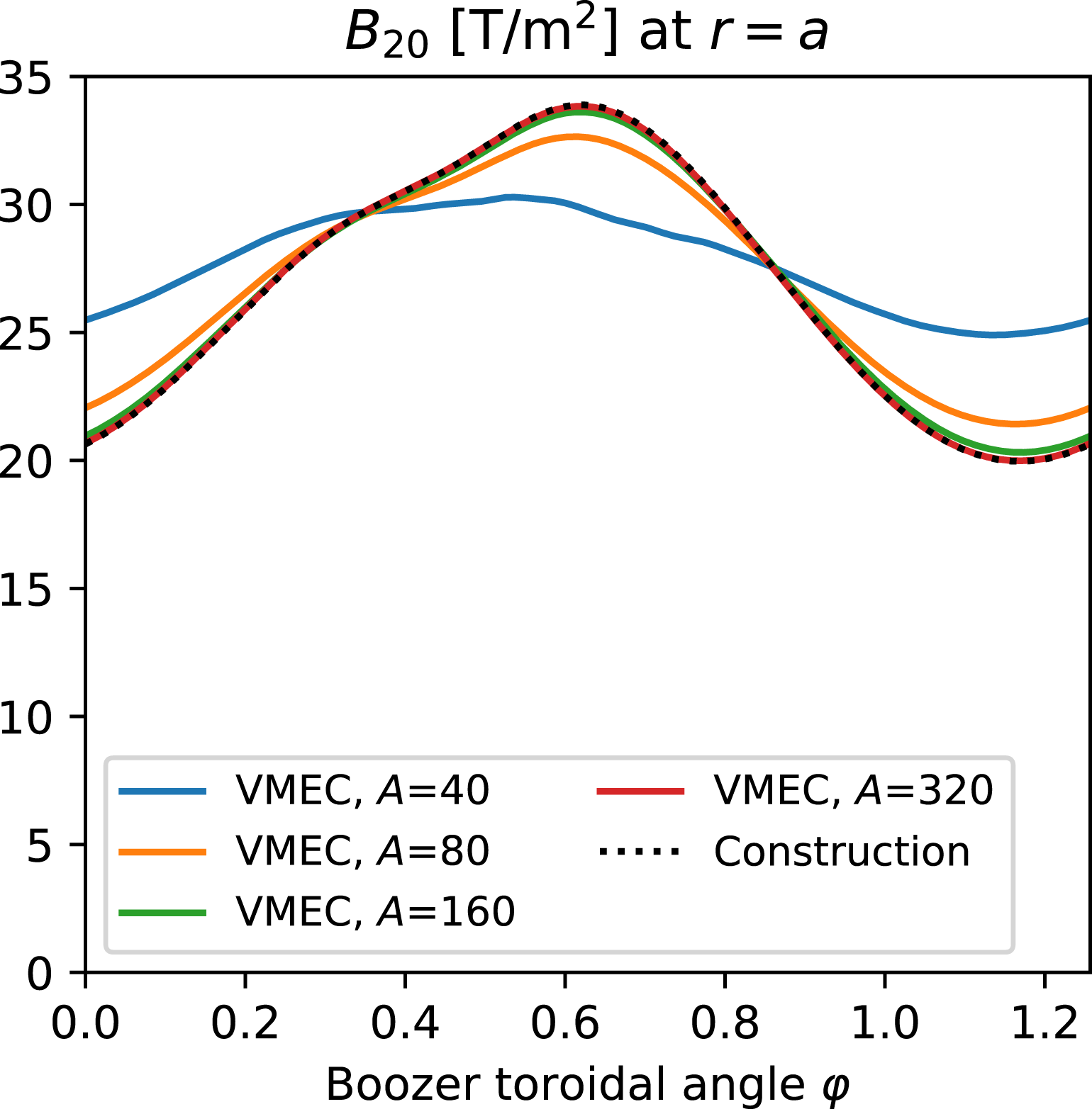
Figure 19. As the aspect ratio
 $A$
increases, the
$A$
increases, the
 $B_{20}(\unicode[STIX]{x1D711})$
component of the field strength of the numerical VMEC configurations converges to the function predicted by the Garren–Boozer construction. Data here are for the non-stellarator-symmetric quasi-helically symmetric configuration of § 5.5.
$B_{20}(\unicode[STIX]{x1D711})$
component of the field strength of the numerical VMEC configurations converges to the function predicted by the Garren–Boozer construction. Data here are for the non-stellarator-symmetric quasi-helically symmetric configuration of § 5.5.
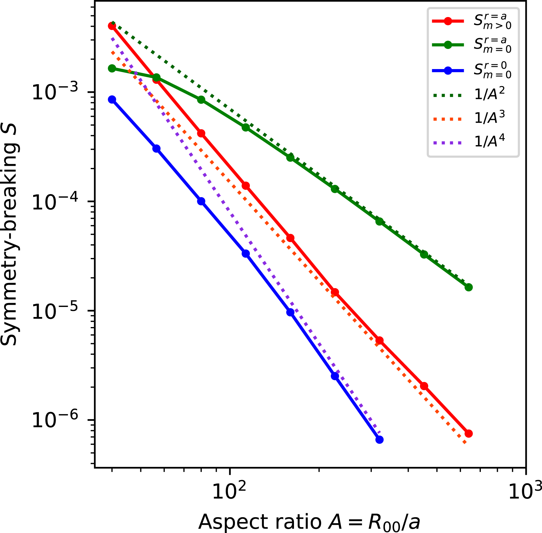
For a final example, we present an example in which all the parameters of the near-axis model are non-zero. This example is limited to quite a large aspect ratio due to the large
 $X_{2}$
and
$X_{2}$
and
 $Y_{2}$
terms, and so is not interesting as an experimental design, but it is useful here as a challenging verification test. We choose the axis shape
$Y_{2}$
terms, and so is not interesting as an experimental design, but it is useful here as a challenging verification test. We choose the axis shape
 $$\begin{eqnarray}\left.\begin{array}{@{}c@{}}R_{0}(\unicode[STIX]{x1D719})~(\text{m})=1+0.3\cos (5\unicode[STIX]{x1D719}),\\ z_{0}(\unicode[STIX]{x1D719})~(\text{m})=0.3\sin (5\unicode[STIX]{x1D719}),\end{array}\right\}\end{eqnarray}$$
which yields quasi-helical symmetry with
 $N=5$
. The other input parameters are chosen to be
$N=5$
. The other input parameters are chosen to be
 $\bar{\unicode[STIX]{x1D702}}=2.5~\text{m}^{-1}$
,
$\bar{\unicode[STIX]{x1D702}}=2.5~\text{m}^{-1}$
,
 $\unicode[STIX]{x1D70E}(0)=0.3$
,
$\unicode[STIX]{x1D70E}(0)=0.3$
,
 $I_{2}=1.6~\text{T}~\text{m}^{-1}$
,
$I_{2}=1.6~\text{T}~\text{m}^{-1}$
,
 $p_{2}=-5\times 10^{6}~\text{Pa}~\text{m}^{-2}$
,
$p_{2}=-5\times 10^{6}~\text{Pa}~\text{m}^{-2}$
,
 $B_{2c}=1~\text{T}~\text{m}^{-2}$
and
$B_{2c}=1~\text{T}~\text{m}^{-2}$
and
 $B_{2s}=3~\text{T}~\text{m}^{-2}$
. Note that stellarator symmetry is broken both by the non-zero value of
$B_{2s}=3~\text{T}~\text{m}^{-2}$
. Note that stellarator symmetry is broken both by the non-zero value of
 $\unicode[STIX]{x1D70E}(0)$
and of
$\unicode[STIX]{x1D70E}(0)$
and of
 $B_{2s}$
. This resulting configuration has
$B_{2s}$
. This resulting configuration has
 $\unicode[STIX]{x1D704}_{0}=0.829$
. The constructed boundary shape is shown in figure 17 for
$\unicode[STIX]{x1D704}_{0}=0.829$
. The constructed boundary shape is shown in figure 17 for
 $A=40$
(
$A=40$
(
 $A_{vmec}=28.5$
), and it can be seen that the surface cross-sections are not stellarator symmetric. The amplitudes of the
$A_{vmec}=28.5$
), and it can be seen that the surface cross-sections are not stellarator symmetric. The amplitudes of the
 $\cos (m\unicode[STIX]{x1D703}-n\unicode[STIX]{x1D711})$
and
$\cos (m\unicode[STIX]{x1D703}-n\unicode[STIX]{x1D711})$
and
 $\sin (m\unicode[STIX]{x1D703}-n\unicode[STIX]{x1D711})$
modes of
$\sin (m\unicode[STIX]{x1D703}-n\unicode[STIX]{x1D711})$
modes of
 $B$
inside this boundary, as computed by VMEC and BOOZ_XFORM, are shown in figure 18. The
$B$
inside this boundary, as computed by VMEC and BOOZ_XFORM, are shown in figure 18. The
 $\cos (\unicode[STIX]{x1D703}-5\unicode[STIX]{x1D711})$
term dominates, as desired, and its amplitude agrees with the prediction of the near-axis equations. Repeating the VMEC and BOOZ_XFORM computations for this solution of the near-axis equations for a range of aspect ratios,
$\cos (\unicode[STIX]{x1D703}-5\unicode[STIX]{x1D711})$
term dominates, as desired, and its amplitude agrees with the prediction of the near-axis equations. Repeating the VMEC and BOOZ_XFORM computations for this solution of the near-axis equations for a range of aspect ratios,
 $[B_{m=0}(\unicode[STIX]{x1D711},r=a)-B(\unicode[STIX]{x1D711},r=0)]/a^{2}$
again converges to the predicted function
$[B_{m=0}(\unicode[STIX]{x1D711},r=a)-B(\unicode[STIX]{x1D711},r=0)]/a^{2}$
again converges to the predicted function
 $B_{20}(\unicode[STIX]{x1D711})$
, as shown in figure 19. Figure 20 shows that the symmetry-breaking modes scale as
$B_{20}(\unicode[STIX]{x1D711})$
, as shown in figure 19. Figure 20 shows that the symmetry-breaking modes scale as
 $1/A^{3}$
or better, as desired, except for the expected
$1/A^{3}$
or better, as desired, except for the expected
 $1/A^{2}$
scaling of
$1/A^{2}$
scaling of
 $S_{m=0}^{r=a}$
associated with the toroidal variation of
$S_{m=0}^{r=a}$
associated with the toroidal variation of
 $B_{20}$
. (The right-most blue points are missing since it did not seem possible to obtain values that were converged with respect to VMEC resolution parameters.) Thus, finite-aspect-ratio VMEC calculations successfully match the near-axis solution even when all parameters of the latter are non-zero.
$B_{20}$
. (The right-most blue points are missing since it did not seem possible to obtain values that were converged with respect to VMEC resolution parameters.) Thus, finite-aspect-ratio VMEC calculations successfully match the near-axis solution even when all parameters of the latter are non-zero.
6 Discussion and conclusions
In this work, we have developed a new and fast method to generate quasisymmetric magnetic fields with sophisticated shaping. In contrast to the traditional approach based on numerical optimization, the approach here uses a reduced set of equations relating the field strength in Boozer coordinates
 $B(r,\unicode[STIX]{x1D703},\unicode[STIX]{x1D711})$
to the three-dimensional shapes of the magnetic surfaces. The shapes that are describable by the
$B(r,\unicode[STIX]{x1D703},\unicode[STIX]{x1D711})$
to the three-dimensional shapes of the magnetic surfaces. The shapes that are describable by the
 $O((r/{\mathcal{R}})^{2})$
near-axis model here are sufficiently general that they can be quite reminiscent of stellarators that have been designed previously using numerical optimization. For instance, the configuration of § 5.2 (figure 5) resembles CFQS (Liu et al.
Reference Liu, Shimizu, Isobe, Okamura, Nishimura, Suzuki, Xu, Zhang, Liu and Huang2018; Shimizu et al.
Reference Shimizu, Liu, Isobe, Okamura, Nishimura, Suzuki, Xu, Zhang, Liu and Huang2018) and the configuration of Henneberg et al. (Reference Henneberg, Drevlak, Nührenberg, Beidler, Turkin, Loizu and Helander2019). Also the configuration of § 5.4 (figure 13) resembles the HSX experiment (Anderson et al.
Reference Anderson, Almagri, Anderson, Matthews, Talmadge and Shohet1995). Despite these similarities, the examples here were generated independently of any previously known configurations. Since these shapes computed by our model are described analytically, they can be parameterized, evaluated rapidly and differentiated. As analytic expressions for the position vector in terms of both Boozer coordinates and cylindrical coordinates (appendix C) are available, one can evaluate virtually any quantity of interest, such as the geometric quantities appearing in the gyrokinetic model of turbulence. Since the system of equations involves only one independent variable (
$O((r/{\mathcal{R}})^{2})$
near-axis model here are sufficiently general that they can be quite reminiscent of stellarators that have been designed previously using numerical optimization. For instance, the configuration of § 5.2 (figure 5) resembles CFQS (Liu et al.
Reference Liu, Shimizu, Isobe, Okamura, Nishimura, Suzuki, Xu, Zhang, Liu and Huang2018; Shimizu et al.
Reference Shimizu, Liu, Isobe, Okamura, Nishimura, Suzuki, Xu, Zhang, Liu and Huang2018) and the configuration of Henneberg et al. (Reference Henneberg, Drevlak, Nührenberg, Beidler, Turkin, Loizu and Helander2019). Also the configuration of § 5.4 (figure 13) resembles the HSX experiment (Anderson et al.
Reference Anderson, Almagri, Anderson, Matthews, Talmadge and Shohet1995). Despite these similarities, the examples here were generated independently of any previously known configurations. Since these shapes computed by our model are described analytically, they can be parameterized, evaluated rapidly and differentiated. As analytic expressions for the position vector in terms of both Boozer coordinates and cylindrical coordinates (appendix C) are available, one can evaluate virtually any quantity of interest, such as the geometric quantities appearing in the gyrokinetic model of turbulence. Since the system of equations involves only one independent variable (
 $\unicode[STIX]{x1D711}$
), compared to three for general MHD equilibrium, the equations here are orders of magnitude faster to solve.
$\unicode[STIX]{x1D711}$
), compared to three for general MHD equilibrium, the equations here are orders of magnitude faster to solve.
Through the examples in § 5, we have demonstrated that the approach here is a practical way to generate and parameterize both quasi-axisymmetric and quasi-helically symmetric configurations. For each of the examples, we showed that the departures from quasisymmetry computed by conventional codes scale with the aspect ratio as expected. In particular, we have demonstrated that quasisymmetry can be achieved (without axisymmetry) to any desired precision, at sufficiently high aspect ratio. Due to the high-order accuracy of the equations in our model, the quality of quasisymmetry can be extremely good. For example, the symmetry-breaking measures (5.2) are smaller than
 $4\times 10^{-7}$
for the rightmost ‘Config 1’ point in figure 4. While at
$4\times 10^{-7}$
for the rightmost ‘Config 1’ point in figure 4. While at
 $A=320$
this configuration is not of great experimental interest, it does represent the most accurate realization of quasisymmetry in a 3-D equilibrium ever reported. While arbitrarily small departures from quasisymmetry can also be obtained with the
$A=320$
this configuration is not of great experimental interest, it does represent the most accurate realization of quasisymmetry in a 3-D equilibrium ever reported. While arbitrarily small departures from quasisymmetry can also be obtained with the
 $O((r/{\mathcal{R}})^{1})$
construction, as demonstrated in figure 4 of Landreman et al. (Reference Landreman, Sengupta and Plunk2019), higher aspect ratios would be required to obtain quasisymmetry to the same precision, due to the weaker scaling of symmetry breaking with
$O((r/{\mathcal{R}})^{1})$
construction, as demonstrated in figure 4 of Landreman et al. (Reference Landreman, Sengupta and Plunk2019), higher aspect ratios would be required to obtain quasisymmetry to the same precision, due to the weaker scaling of symmetry breaking with
 $1/A^{2}$
in that case. As an additional demonstration of the high accuracy to which quasisymmetry can be achieved by the
$1/A^{2}$
in that case. As an additional demonstration of the high accuracy to which quasisymmetry can be achieved by the
 $O((r/{\mathcal{R}})^{2})$
construction, figure 21 shows the contours of
$O((r/{\mathcal{R}})^{2})$
construction, figure 21 shows the contours of
 $B$
on the boundary surfaces of the configurations of §§ 5.2 and 5.4 with aspect ratios chosen by the following criterion: at a reactor-relevant mean field
$B$
on the boundary surfaces of the configurations of §§ 5.2 and 5.4 with aspect ratios chosen by the following criterion: at a reactor-relevant mean field
 $B_{0,0}=5$
T, the largest quasisymmetry-breaking Fourier mode amplitudes are only 0.5 Gauss, the approximate magnitude of Earth’s magnetic field. This condition results in aspect ratios
$B_{0,0}=5$
T, the largest quasisymmetry-breaking Fourier mode amplitudes are only 0.5 Gauss, the approximate magnitude of Earth’s magnetic field. This condition results in aspect ratios
 $A_{vmec}\sim$
80. There may be other configurations for which this condition can be met at lower aspect ratio; our goal here is merely to demonstrate that the condition can indeed be achieved. The deviation from symmetry is nearly invisible in figure 21, and the
$A_{vmec}\sim$
80. There may be other configurations for which this condition can be met at lower aspect ratio; our goal here is merely to demonstrate that the condition can indeed be achieved. The deviation from symmetry is nearly invisible in figure 21, and the
 $B$
contours are far more quasisymmetric than in other nominally quasisymmetric configurations reported previously, e.g. figures 5–7 of Beidler et al. (Reference Beidler, Allmaier, Isaev, Kasilov, Kernbichler, Leitold, Maassberg, Mikkelsen, Murakami and Schmidt2011).
$B$
contours are far more quasisymmetric than in other nominally quasisymmetric configurations reported previously, e.g. figures 5–7 of Beidler et al. (Reference Beidler, Allmaier, Isaev, Kasilov, Kernbichler, Leitold, Maassberg, Mikkelsen, Murakami and Schmidt2011).
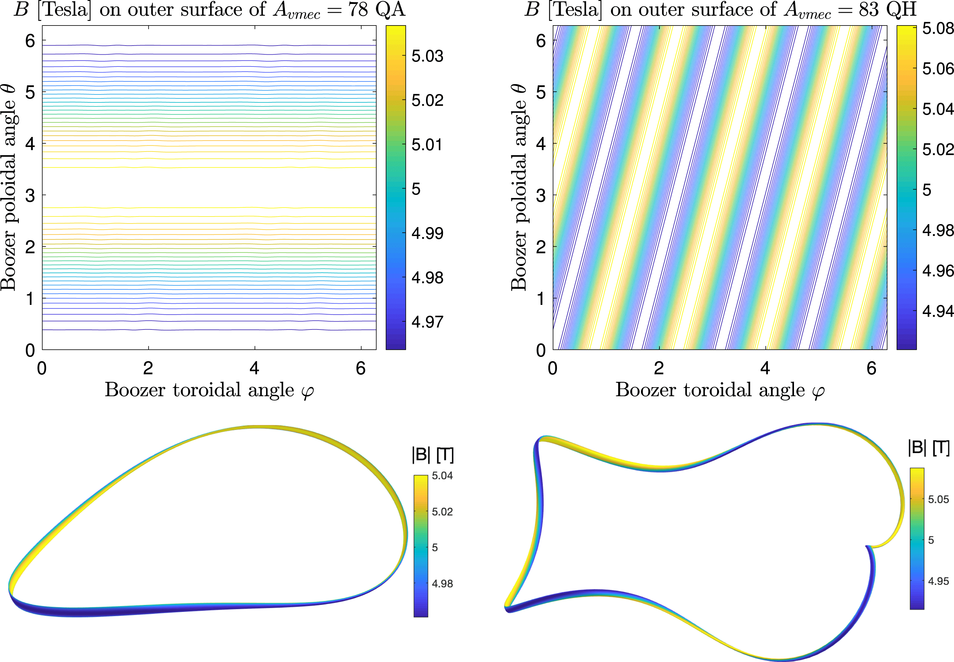
Figure 21. Contours of
 $B(\unicode[STIX]{x1D703},\unicode[STIX]{x1D701})$
at the boundaries of the configurations of §§ 5.2 and 5.4, scaled to a mean field of 5 Tesla, at the aspect ratio for which the largest symmetry-breaking Fourier modes have amplitude
$B(\unicode[STIX]{x1D703},\unicode[STIX]{x1D701})$
at the boundaries of the configurations of §§ 5.2 and 5.4, scaled to a mean field of 5 Tesla, at the aspect ratio for which the largest symmetry-breaking Fourier modes have amplitude
 $0.5$
Gauss, the magnitude of Earth’s magnetic field. Departures from quasisymmetry are nearly imperceptible on the scale of the plots, demonstrating that quasisymmetry can be realized in strongly non-axisymmetric equilibria to very high accuracy, at least at high
$0.5$
Gauss, the magnitude of Earth’s magnetic field. Departures from quasisymmetry are nearly imperceptible on the scale of the plots, demonstrating that quasisymmetry can be realized in strongly non-axisymmetric equilibria to very high accuracy, at least at high
 $A$
.
$A$
.
Most of the solutions exhibited in this paper have a relatively high aspect ratio, which is not surprising since the method is based on an expansion in aspect ratio. Several methods are likely to enable configurations of lower aspect ratio to be generated. First, by including more Fourier modes in the axis shape,
 $X_{2}$
and
$X_{2}$
and
 $Y_{2}$
could perhaps be further reduced, resulting in configurations for which the
$Y_{2}$
could perhaps be further reduced, resulting in configurations for which the
 $O((r/{\mathcal{R}})^{3})$
symmetry-breaking terms have a smaller leading constant. Second, the method of § 4.4 of Landreman et al. (Reference Landreman, Sengupta and Plunk2019) could be used to extrapolate outward from a high-
$O((r/{\mathcal{R}})^{3})$
symmetry-breaking terms have a smaller leading constant. Second, the method of § 4.4 of Landreman et al. (Reference Landreman, Sengupta and Plunk2019) could be used to extrapolate outward from a high-
 $A$
configuration while preserving good quasisymmetry in the core. Third, a large value of
$A$
configuration while preserving good quasisymmetry in the core. Third, a large value of
 $a$
could be used in the present approach, resulting in moderate deviations from quasisymmetry, which could then be reduced by conventional optimization. Lastly, a configuration with smaller
$a$
could be used in the present approach, resulting in moderate deviations from quasisymmetry, which could then be reduced by conventional optimization. Lastly, a configuration with smaller
 $a$
and good quasisymmetry generated by the construction here could be used to initialize conventional optimization, in which the aspect ratio is included in the objective function for minimization.
$a$
and good quasisymmetry generated by the construction here could be used to initialize conventional optimization, in which the aspect ratio is included in the objective function for minimization.
The work here suggests many avenues for future study, some of which are enumerated here. (i) It was shown previously that practical quasisymmetric configurations obtained by optimization closely match the
 $O(r/{\mathcal{R}})$
near-axis construction (Landreman Reference Landreman2019), and the comparison should be repeated for the
$O(r/{\mathcal{R}})$
near-axis construction (Landreman Reference Landreman2019), and the comparison should be repeated for the
 $O((r/{\mathcal{R}})^{2})$
model. (ii) An efficient procedure should be found to solve for model parameters such that
$O((r/{\mathcal{R}})^{2})$
model. (ii) An efficient procedure should be found to solve for model parameters such that
 $B_{20}$
is independent of
$B_{20}$
is independent of
 $\unicode[STIX]{x1D711}$
. (iii) While a precise understanding exists of the solution space for
$\unicode[STIX]{x1D711}$
. (iii) While a precise understanding exists of the solution space for
 $O(r/{\mathcal{R}})$
quasisymmetry (Landreman et al.
Reference Landreman, Sengupta and Plunk2019), the same insight has yet to be developed for the
$O(r/{\mathcal{R}})$
quasisymmetry (Landreman et al.
Reference Landreman, Sengupta and Plunk2019), the same insight has yet to be developed for the
 $O((r/{\mathcal{R}})^{2})$
model. It would be valuable to understand the space of solutions to the
$O((r/{\mathcal{R}})^{2})$
model. It would be valuable to understand the space of solutions to the
 $O((r/{\mathcal{R}})^{2})$
model to be sure all the interesting regions of parameter space have been identified. (iv) It was seen here that some toroidal variation of
$O((r/{\mathcal{R}})^{2})$
model to be sure all the interesting regions of parameter space have been identified. (iv) It was seen here that some toroidal variation of
 $B_{20}$
could be allowed without
$B_{20}$
could be allowed without
 $B_{20}$
becoming the dominant quasisymmetry-breaking mode, so the effect of allowing small toroidal variation of
$B_{20}$
becoming the dominant quasisymmetry-breaking mode, so the effect of allowing small toroidal variation of
 $B_{2c}$
or
$B_{2c}$
or
 $B_{2s}$
should be examined. (v) It should be investigated whether quasisymmetry could be optimized off-axis, by introducing small toroidal variation in
$B_{2s}$
should be examined. (v) It should be investigated whether quasisymmetry could be optimized off-axis, by introducing small toroidal variation in
 $B_{0}$
that is cancelled by
$B_{0}$
that is cancelled by
 $B_{20}$
at a certain radius. (vi) The space of configurations that are omnigenous to
$B_{20}$
at a certain radius. (vi) The space of configurations that are omnigenous to
 $O(r/{\mathcal{R}})$
was recently examined (Plunk et al.
Reference Plunk, Landreman and Helander2019), and the analysis could possibly be extended to
$O(r/{\mathcal{R}})$
was recently examined (Plunk et al.
Reference Plunk, Landreman and Helander2019), and the analysis could possibly be extended to
 $O((r/{\mathcal{R}})^{2})$
omnigenity using results derived here.
$O((r/{\mathcal{R}})^{2})$
omnigenity using results derived here.
Finally, extensions of the quasisymmetry model here to even higher order in
 $r$
could be pursued. One motivation for such an extension is that global magnetic shear first appears at
$r$
could be pursued. One motivation for such an extension is that global magnetic shear first appears at
 $O((r/{\mathcal{R}})^{3})$
. Although quasisymmetry cannot generally be achieved through
$O((r/{\mathcal{R}})^{3})$
. Although quasisymmetry cannot generally be achieved through
 $O((r/{\mathcal{R}})^{3})$
(Garren & Boozer Reference Garren and Boozer1991a
), the size of the
$O((r/{\mathcal{R}})^{3})$
(Garren & Boozer Reference Garren and Boozer1991a
), the size of the
 $O((r/{\mathcal{R}})^{3})$
terms informs how rapidly quasisymmetry degrades with
$O((r/{\mathcal{R}})^{3})$
terms informs how rapidly quasisymmetry degrades with
 $r$
, so solutions could be sought in which these terms were minimized.
$r$
, so solutions could be sought in which these terms were minimized.
Acknowledgements
This work was supported by the U.S. Department of Energy, Office of Science, Office of Fusion Energy Science, under award nos DE-FG02-93ER54197 and DE-FG02-86ER53223. This work was also supported by a grant from the Simons Foundation (560651, M.L.).
Appendix A. Derivation of the equations at each order
In this section we elaborate on § 2, showing a streamlined method to derive the required equations at each order in
 $r/{\mathcal{R}}$
. It is possible to obtain the same final equations without the manipulations of § A.1, but at the cost of substantial additional algebra. In particular, to derive the equations for
$r/{\mathcal{R}}$
. It is possible to obtain the same final equations without the manipulations of § A.1, but at the cost of substantial additional algebra. In particular, to derive the equations for
 $\{X_{j},Y_{j},Z_{j}\}$
at a given order
$\{X_{j},Y_{j},Z_{j}\}$
at a given order
 $j$
without these manipulations, it would be necessary to first derive equations involving
$j$
without these manipulations, it would be necessary to first derive equations involving
 $Z_{j+1}$
, and then form linear combinations to eliminate this higher-order quantity. The method of § A.1 enables the equations for
$Z_{j+1}$
, and then form linear combinations to eliminate this higher-order quantity. The method of § A.1 enables the equations for
 $\{X_{j},Y_{j},Z_{j}\}$
to be obtained directly without introducing
$\{X_{j},Y_{j},Z_{j}\}$
to be obtained directly without introducing
 $Z_{j+1}$
.
$Z_{j+1}$
.
A.1 Fundamental equations
To begin, note the product of (2.2) and (2.3) gives the inverse Jacobian
 $$\begin{eqnarray}\unicode[STIX]{x1D735}\unicode[STIX]{x1D713}\boldsymbol{\cdot }\unicode[STIX]{x1D735}\unicode[STIX]{x1D717}\times \unicode[STIX]{x1D735}\unicode[STIX]{x1D711}=\frac{1}{\sqrt{g}}=\frac{B^{2}}{G+\unicode[STIX]{x1D704}I}.\end{eqnarray}$$
Then, from (2.2) and (2.3), applying (2.5)–(2.6) and using
 $\unicode[STIX]{x2202}/\unicode[STIX]{x2202}\unicode[STIX]{x1D713}=(r\bar{B})^{-1}\unicode[STIX]{x2202}/\unicode[STIX]{x2202}r$
, we obtain the following three scalar equations:
$\unicode[STIX]{x2202}/\unicode[STIX]{x2202}\unicode[STIX]{x1D713}=(r\bar{B})^{-1}\unicode[STIX]{x2202}/\unicode[STIX]{x2202}r$
, we obtain the following three scalar equations:
 $$\begin{eqnarray}\displaystyle & \displaystyle \{Y,Z\}=T_{X}, & \displaystyle\end{eqnarray}$$
 $$\begin{eqnarray}\displaystyle & \displaystyle \{Z,X\}=T_{Y}, & \displaystyle\end{eqnarray}$$
 $$\begin{eqnarray}\displaystyle & \displaystyle \{X,Y\}=T_{Z}, & \displaystyle\end{eqnarray}$$
where
 $\{\ldots ,\ldots \}$
denotes a Poisson bracket in the
$\{\ldots ,\ldots \}$
denotes a Poisson bracket in the
 $(r,\unicode[STIX]{x1D717})$
coordinates,
$(r,\unicode[STIX]{x1D717})$
coordinates,
 $$\begin{eqnarray}\{X,Y\}=\frac{\unicode[STIX]{x2202}X}{\unicode[STIX]{x2202}r}\frac{\unicode[STIX]{x2202}Y}{\unicode[STIX]{x2202}\unicode[STIX]{x1D717}}-\frac{\unicode[STIX]{x2202}X}{\unicode[STIX]{x2202}\unicode[STIX]{x1D717}}\frac{\unicode[STIX]{x2202}Y}{\unicode[STIX]{x2202}r}.\end{eqnarray}$$
The right-hand sides of (A 2)–(A 4) are
 $$\begin{eqnarray}\displaystyle & \displaystyle T_{X}=\frac{1}{G+NI}\left[r\bar{B}\left(\unicode[STIX]{x1D6EF}+\unicode[STIX]{x1D704}_{N}\frac{\unicode[STIX]{x2202}X}{\unicode[STIX]{x2202}\unicode[STIX]{x1D717}}\right)-I\left(\unicode[STIX]{x1D6F6}\frac{\unicode[STIX]{x2202}Z}{\unicode[STIX]{x2202}r}-\unicode[STIX]{x1D6EC}\frac{\unicode[STIX]{x2202}Y}{\unicode[STIX]{x2202}r}\right)-\unicode[STIX]{x1D6FD}r\bar{B}\left(\unicode[STIX]{x1D6EC}\frac{\unicode[STIX]{x2202}Y}{\unicode[STIX]{x2202}\unicode[STIX]{x1D717}}-\unicode[STIX]{x1D6F6}\frac{\unicode[STIX]{x2202}Z}{\unicode[STIX]{x2202}\unicode[STIX]{x1D717}}\right)\right], & \displaystyle \nonumber\\ \displaystyle & & \displaystyle\end{eqnarray}$$
 $$\begin{eqnarray}\displaystyle & \displaystyle T_{Y}=\frac{1}{G+NI}\left[r\bar{B}\left(\unicode[STIX]{x1D6F6}+\unicode[STIX]{x1D704}_{N}\frac{\unicode[STIX]{x2202}Y}{\unicode[STIX]{x2202}\unicode[STIX]{x1D717}}\right)-I\left(\unicode[STIX]{x1D6EC}\frac{\unicode[STIX]{x2202}X}{\unicode[STIX]{x2202}r}-\unicode[STIX]{x1D6EF}\frac{\unicode[STIX]{x2202}Z}{\unicode[STIX]{x2202}r}\right)-\unicode[STIX]{x1D6FD}r\bar{B}\left(\unicode[STIX]{x1D6EF}\frac{\unicode[STIX]{x2202}Z}{\unicode[STIX]{x2202}\unicode[STIX]{x1D717}}-\unicode[STIX]{x1D6EC}\frac{\unicode[STIX]{x2202}X}{\unicode[STIX]{x2202}\unicode[STIX]{x1D717}}\right)\right], & \displaystyle \nonumber\\ \displaystyle & & \displaystyle\end{eqnarray}$$
and
 $$\begin{eqnarray}T_{Z}=\frac{1}{G+NI}\left[r\bar{B}\left(\unicode[STIX]{x1D6EC}+\unicode[STIX]{x1D704}_{N}\frac{\unicode[STIX]{x2202}Z}{\unicode[STIX]{x2202}\unicode[STIX]{x1D717}}\right)-I\left(\unicode[STIX]{x1D6EF}\frac{\unicode[STIX]{x2202}Y}{\unicode[STIX]{x2202}r}-\unicode[STIX]{x1D6F6}\frac{\unicode[STIX]{x2202}X}{\unicode[STIX]{x2202}r}\right)-\unicode[STIX]{x1D6FD}r\bar{B}\left(\unicode[STIX]{x1D6F6}\frac{\unicode[STIX]{x2202}X}{\unicode[STIX]{x2202}\unicode[STIX]{x1D717}}-\unicode[STIX]{x1D6EF}\frac{\unicode[STIX]{x2202}Y}{\unicode[STIX]{x2202}\unicode[STIX]{x1D717}}\right)\right],\end{eqnarray}$$
where
 $$\begin{eqnarray}\displaystyle & \displaystyle \unicode[STIX]{x1D6EC}=\frac{\unicode[STIX]{x2202}Z}{\unicode[STIX]{x2202}\unicode[STIX]{x1D711}}+(1-X\unicode[STIX]{x1D705})\ell ^{\prime }, & \displaystyle\end{eqnarray}$$
 $$\begin{eqnarray}\displaystyle & \displaystyle \unicode[STIX]{x1D6EF}=\frac{\unicode[STIX]{x2202}X}{\unicode[STIX]{x2202}\unicode[STIX]{x1D711}}+(-Y\unicode[STIX]{x1D70F}+Z\unicode[STIX]{x1D705})\ell ^{\prime }, & \displaystyle\end{eqnarray}$$
 $$\begin{eqnarray}\displaystyle & \displaystyle \unicode[STIX]{x1D6F6}=\frac{\unicode[STIX]{x2202}Y}{\unicode[STIX]{x2202}\unicode[STIX]{x1D711}}+X\unicode[STIX]{x1D70F}\ell ^{\prime }, & \displaystyle\end{eqnarray}$$
and
 $\ell ^{\prime }=\sqrt{(\text{d}\boldsymbol{ r}_{0}/\text{d}\unicode[STIX]{x1D711})^{2}}$
.
$\ell ^{\prime }=\sqrt{(\text{d}\boldsymbol{ r}_{0}/\text{d}\unicode[STIX]{x1D711})^{2}}$
.
As alluded to above, it turns out to be inconvenient to solve (A 2) and (A 3) as written, since these equations involve
 $Z$
to one higher order than
$Z$
to one higher order than
 $X$
or
$X$
or
 $Y$
. The reason is that
$Y$
. The reason is that
 $X_{1}$
and
$X_{1}$
and
 $Y_{1}$
are non-zero while
$Y_{1}$
are non-zero while
 $Z_{1}$
turns out to vanish (shown in the next subsection), so the left-hand sides at
$Z_{1}$
turns out to vanish (shown in the next subsection), so the left-hand sides at
 $O((r/{\mathcal{R}})^{j}r)$
include terms
$O((r/{\mathcal{R}})^{j}r)$
include terms
 $\{rY_{1},r^{j+1}Z_{j+1}\}$
and
$\{rY_{1},r^{j+1}Z_{j+1}\}$
and
 $\{r^{j+1}Z_{j+1},rX_{1}\}$
, while the highest orders of
$\{r^{j+1}Z_{j+1},rX_{1}\}$
, while the highest orders of
 $X$
and
$X$
and
 $Y$
appear through
$Y$
appear through
 $\{r^{\,j}Y_{j},r^{2}Z_{2}\}$
and
$\{r^{\,j}Y_{j},r^{2}Z_{2}\}$
and
 $\{r^{2}Z_{2},r^{\,j}X_{j}\}$
. Therefore it turns out to be convenient to form two combinations of (A 2) and (A 3), one in which
$\{r^{2}Z_{2},r^{\,j}X_{j}\}$
. Therefore it turns out to be convenient to form two combinations of (A 2) and (A 3), one in which
 $Z$
is given explicitly in terms of lower-order quantities, and the other in which the higher-order
$Z$
is given explicitly in terms of lower-order quantities, and the other in which the higher-order
 $Z$
terms are eliminated to give a constraint on the lower-order quantities. To form the first desired combination, we start by writing (A 2)–(A 3) as
$Z$
terms are eliminated to give a constraint on the lower-order quantities. To form the first desired combination, we start by writing (A 2)–(A 3) as
 $$\begin{eqnarray}\left(\begin{array}{@{}cc@{}}-\unicode[STIX]{x2202}Y/\unicode[STIX]{x2202}\unicode[STIX]{x1D717} & \unicode[STIX]{x2202}Y/\unicode[STIX]{x2202}r\\ \unicode[STIX]{x2202}X/\unicode[STIX]{x2202}\unicode[STIX]{x1D717} & -\unicode[STIX]{x2202}X/\unicode[STIX]{x2202}r\end{array}\right)\left(\begin{array}{@{}c@{}}\unicode[STIX]{x2202}Z/\unicode[STIX]{x2202}r\\ \unicode[STIX]{x2202}Z/\unicode[STIX]{x2202}\unicode[STIX]{x1D717}\end{array}\right)=\left(\begin{array}{@{}c@{}}T_{X}\\ T_{Y}\end{array}\right).\end{eqnarray}$$
This linear system can be solved to give
 $$\begin{eqnarray}\left(\begin{array}{@{}c@{}}\unicode[STIX]{x2202}Z/\unicode[STIX]{x2202}r\\ \unicode[STIX]{x2202}Z/\unicode[STIX]{x2202}\unicode[STIX]{x1D717}\end{array}\right)=-\left[\frac{\unicode[STIX]{x2202}X}{\unicode[STIX]{x2202}r}\frac{\unicode[STIX]{x2202}Y}{\unicode[STIX]{x2202}\unicode[STIX]{x1D717}}-\frac{\unicode[STIX]{x2202}X}{\unicode[STIX]{x2202}\unicode[STIX]{x1D717}}\frac{\unicode[STIX]{x2202}Y}{\unicode[STIX]{x2202}r}\right]^{-1}\left(\begin{array}{@{}cc@{}}\unicode[STIX]{x2202}X/\unicode[STIX]{x2202}r & \unicode[STIX]{x2202}Y/\unicode[STIX]{x2202}r\\ \unicode[STIX]{x2202}X/\unicode[STIX]{x2202}\unicode[STIX]{x1D717} & \unicode[STIX]{x2202}Y/\unicode[STIX]{x2202}\unicode[STIX]{x1D717}\end{array}\right)\left(\begin{array}{@{}c@{}}T_{X}\\ T_{Y}\end{array}\right),\end{eqnarray}$$
where the determinant can be recognized from (A 4) as
 $T_{Z}$
. The top row of (A 13) then gives an equation that will tell us
$T_{Z}$
. The top row of (A 13) then gives an equation that will tell us
 $Z$
at each order in terms of lower-order quantities,
$Z$
at each order in terms of lower-order quantities,
 $$\begin{eqnarray}\frac{\unicode[STIX]{x2202}Z}{\unicode[STIX]{x2202}r}=-\frac{1}{T_{Z}}\left(\frac{\unicode[STIX]{x2202}X}{\unicode[STIX]{x2202}r}T_{X}+\frac{\unicode[STIX]{x2202}Y}{\unicode[STIX]{x2202}r}T_{Y}\right).\end{eqnarray}$$
The equality of mixed partial derivatives
 $\unicode[STIX]{x2202}^{2}Z/\unicode[STIX]{x2202}r\unicode[STIX]{x2202}\unicode[STIX]{x1D717}=\unicode[STIX]{x2202}^{2}Z/\unicode[STIX]{x2202}\unicode[STIX]{x1D717}\unicode[STIX]{x2202}r$
can be used with (A 13) to obtain
$\unicode[STIX]{x2202}^{2}Z/\unicode[STIX]{x2202}r\unicode[STIX]{x2202}\unicode[STIX]{x1D717}=\unicode[STIX]{x2202}^{2}Z/\unicode[STIX]{x2202}\unicode[STIX]{x1D717}\unicode[STIX]{x2202}r$
can be used with (A 13) to obtain
 $$\begin{eqnarray}\{X,T_{X}/T_{Z}\}+\{Y,T_{Y}/T_{Z}\}=0.\end{eqnarray}$$
This latter equation is the second desired combination of (A 2) and (A 3), giving a constraint on
 $X$
and
$X$
and
 $Y$
at each order without introducing
$Y$
at each order without introducing
 $Z$
at the next order.
$Z$
at the next order.
We can also derive a different combination of (A 2) and (A 3) with the same property, as an equivalent alternative to (A 15), which more closely corresponds to the equations of Garren and Boozer at
 $O((r/{\mathcal{R}})^{2})$
. This second approach begins with the observation that the problematic terms that introduce
$O((r/{\mathcal{R}})^{2})$
. This second approach begins with the observation that the problematic terms that introduce
 $Z$
at higher order than
$Z$
at higher order than
 $X$
and
$X$
and
 $Y$
are
$Y$
are
 $\{rY_{1},r^{j+1}Z_{j+1}\}$
and
$\{rY_{1},r^{j+1}Z_{j+1}\}$
and
 $\{r^{j+1}Z_{j+1},rX_{1}\}$
. To separate out these terms, we introduce
$\{r^{j+1}Z_{j+1},rX_{1}\}$
. To separate out these terms, we introduce
 $X_{{>}1}=X-rX_{1}$
and
$X_{{>}1}=X-rX_{1}$
and
 $Y_{{>}1}=Y-rY_{1}$
, so (A 2)–(A 3) give
$Y_{{>}1}=Y-rY_{1}$
, so (A 2)–(A 3) give
 $$\begin{eqnarray}T_{X}-\{rY_{1},Z\}-\{Y_{{>}1},Z\}=0,\quad T_{Y}-\{Z,rX_{1}\}-\{Z,X_{{>}1}\}=0.\end{eqnarray}$$
We look for a combination of these equations in which the problematic terms
 $\{rY_{1},Z\}$
and
$\{rY_{1},Z\}$
and
 $\{Z,rX_{1}\}$
are annihilated. To this end, it can be verified that
$\{Z,rX_{1}\}$
are annihilated. To this end, it can be verified that
 $$\begin{eqnarray}\{rX_{1},\{rY_{1},Z\}/r\}+\{rY_{1},\{Z,rX_{1}\}/r\}=0.\end{eqnarray}$$
Forming the analogous combination of (A 16) then gives the desired relation, in which
 $Z$
appears at no higher order than
$Z$
appears at no higher order than
 $X$
or
$X$
or
 $Y$
,
$Y$
,
 $$\begin{eqnarray}\left\{rX_{1},\frac{T_{X}-\{Y_{{>}1},Z\}}{r}\right\}+\left\{rY_{1},\frac{T_{Y}-\{Z,X_{{>}1}\}}{r}\right\}=0.\end{eqnarray}$$
Finally, we obtain an expression for the magnetic field strength by squaring (2.2), and using (A 1),
 $$\begin{eqnarray}\frac{(G+\unicode[STIX]{x1D704}I)^{2}}{B^{2}}=\left(\unicode[STIX]{x1D6EC}+\unicode[STIX]{x1D704}_{N}\frac{\unicode[STIX]{x2202}Z}{\unicode[STIX]{x2202}\unicode[STIX]{x1D717}}\right)^{2}+\left(\unicode[STIX]{x1D6EF}+\unicode[STIX]{x1D704}_{N}\frac{\unicode[STIX]{x2202}X}{\unicode[STIX]{x2202}\unicode[STIX]{x1D717}}\right)^{2}+\left(\unicode[STIX]{x1D6F6}+\unicode[STIX]{x1D704}_{N}\frac{\unicode[STIX]{x2202}Y}{\unicode[STIX]{x2202}\unicode[STIX]{x1D717}}\right)^{2}.\end{eqnarray}$$
Equations (A 4), (A 14), (A 18) and (A 19) are the four equations we will solve at each order for the corresponding unknowns
 $X$
,
$X$
,
 $Y$
,
$Y$
,
 $Z$
and
$Z$
and
 $B$
.
$B$
.
A.2 Equations through
$O((r/{\mathcal{R}})^{2})$

We now evaluate the first few orders of the
 $r/{\mathcal{R}}$
expansion, without assuming quasisymmetry. At
$r/{\mathcal{R}}$
expansion, without assuming quasisymmetry. At
 $O((r/{\mathcal{R}})^{0})$
, (A 19) gives
$O((r/{\mathcal{R}})^{0})$
, (A 19) gives
 $$\begin{eqnarray}G_{0}=s_{G}B_{0}\ell ^{\prime },\end{eqnarray}$$
where
 $s_{G}=\pm 1=\text{sign}(G_{0})$
, and (A 14) gives
$s_{G}=\pm 1=\text{sign}(G_{0})$
, and (A 14) gives
 $Z_{1}=0$
. Equations (A 4) and (A 18) have no terms of this order. At
$Z_{1}=0$
. Equations (A 4) and (A 18) have no terms of this order. At
 $O((r/{\mathcal{R}})^{1})$
, (A 4) gives
$O((r/{\mathcal{R}})^{1})$
, (A 4) gives
 $$\begin{eqnarray}X_{1c}Y_{1s}-X_{1s}Y_{1c}=\frac{s_{G}\bar{B}}{B_{0}},\end{eqnarray}$$
the
 $\sin \unicode[STIX]{x1D717}$
and
$\sin \unicode[STIX]{x1D717}$
and
 $\cos \unicode[STIX]{x1D717}$
modes of (A 19) give
$\cos \unicode[STIX]{x1D717}$
modes of (A 19) give
 $$\begin{eqnarray}B_{1s}=\unicode[STIX]{x1D705}X_{1s}B_{0},\quad B_{1c}=\unicode[STIX]{x1D705}X_{1c}B_{0},\end{eqnarray}$$
and (A 18) gives
 $$\begin{eqnarray}\unicode[STIX]{x1D704}_{N0}V_{1}=X_{1c}X_{1s}^{\prime }-X_{1s}X_{1c}^{\prime }+Y_{1c}Y_{1s}^{\prime }-Y_{1s}Y_{1c}^{\prime }+2\left(\frac{I_{2}}{\bar{B}}-\unicode[STIX]{x1D70F}\right)\frac{G_{0}\bar{B}}{B_{0}^{2}},\end{eqnarray}$$
where primes denote
 $\text{d}/\text{d}\unicode[STIX]{x1D711}$
and
$\text{d}/\text{d}\unicode[STIX]{x1D711}$
and
 $$\begin{eqnarray}V_{1}=X_{1s}^{2}+X_{1c}^{2}+Y_{1s}^{2}+Y_{1c}^{2}.\end{eqnarray}$$
It is convenient to introduce
 $\unicode[STIX]{x1D70E}(\unicode[STIX]{x1D711})=(B_{1s}Y_{1s}+B_{1c}Y_{1c})/(s_{G}\bar{B}\unicode[STIX]{x1D705})$
, in which case (A 21)–(A 22) imply
$\unicode[STIX]{x1D70E}(\unicode[STIX]{x1D711})=(B_{1s}Y_{1s}+B_{1c}Y_{1c})/(s_{G}\bar{B}\unicode[STIX]{x1D705})$
, in which case (A 21)–(A 22) imply
 $$\begin{eqnarray}Y_{1s}=\frac{(B_{1c}+B_{1s}\unicode[STIX]{x1D70E})s_{G}\bar{B}\unicode[STIX]{x1D705}}{B_{1s}^{2}+B_{1c}^{2}},\quad Y_{1c}=\frac{(-B_{1s}+B_{1c}\unicode[STIX]{x1D70E})s_{G}\bar{B}\unicode[STIX]{x1D705}}{B_{1s}^{2}+B_{1c}^{2}},\end{eqnarray}$$
and (A 23)–(A 24) can be written
 $$\begin{eqnarray}\displaystyle & & \displaystyle \unicode[STIX]{x1D70E}^{\prime }+\left[\frac{(B_{1s}^{2}+B_{1c}^{2})^{2}}{B_{0}^{2}\bar{B}^{2}\unicode[STIX]{x1D705}^{4}}+1+\unicode[STIX]{x1D70E}^{2}\right]\left[\unicode[STIX]{x1D704}_{N0}+\frac{B_{1s}B_{1c}^{\prime }-B_{1c}B_{1s}^{\prime }}{B_{1s}^{2}+B_{1c}^{2}}\right]\nonumber\\ \displaystyle & & \displaystyle \quad -\,2\left(\frac{I_{2}}{\bar{B}}-\unicode[STIX]{x1D70F}\right)\frac{G_{0}\left(B_{1s}^{2}+B_{1c}^{2}\right)}{\bar{B}B_{0}^{2}\unicode[STIX]{x1D705}^{2}}=0.\end{eqnarray}$$
Next, the
 $\unicode[STIX]{x1D717}$
-independent,
$\unicode[STIX]{x1D717}$
-independent,
 $\sin 2\unicode[STIX]{x1D717}$
and
$\sin 2\unicode[STIX]{x1D717}$
and
 $\cos 2\unicode[STIX]{x1D717}$
modes of (A 14) give
$\cos 2\unicode[STIX]{x1D717}$
modes of (A 14) give
 $$\begin{eqnarray}\displaystyle & \displaystyle Z_{20}=\frac{\unicode[STIX]{x1D6FD}_{0}\bar{B}\ell ^{\prime }}{2G_{0}}-\frac{V_{1}^{\prime }}{8\ell ^{\prime }}, & \displaystyle\end{eqnarray}$$
 $$\begin{eqnarray}\displaystyle & \displaystyle Z_{2s}=-\frac{1}{8\ell ^{\prime }}(V_{2}^{\prime }-2\unicode[STIX]{x1D704}_{N0}V_{3}), & \displaystyle\end{eqnarray}$$
 $$\begin{eqnarray}\displaystyle & \displaystyle Z_{2c}=-\frac{1}{8\ell ^{\prime }}(V_{3}^{\prime }+2\unicode[STIX]{x1D704}_{N0}V_{2}), & \displaystyle\end{eqnarray}$$
where
 $$\begin{eqnarray}\displaystyle & \displaystyle V_{2}=2[X_{1s}X_{1c}+Y_{1s}Y_{1c}], & \displaystyle\end{eqnarray}$$
 $$\begin{eqnarray}\displaystyle & \displaystyle V_{3}=X_{1c}^{2}-X_{1s}^{2}+Y_{1c}^{2}-Y_{1s}^{2}. & \displaystyle\end{eqnarray}$$
At
 $O((r/{\mathcal{R}})^{2})$
, the
$O((r/{\mathcal{R}})^{2})$
, the
 $\sin \unicode[STIX]{x1D717}$
and
$\sin \unicode[STIX]{x1D717}$
and
 $\cos \unicode[STIX]{x1D717}$
terms of (A 4) are
$\cos \unicode[STIX]{x1D717}$
terms of (A 4) are
 $$\begin{eqnarray}\displaystyle & \displaystyle -\frac{s_{G}\bar{B}}{2B_{0}}X_{1s}\unicode[STIX]{x1D705}=-X_{1s}Y_{2s}-X_{1c}Y_{2c}+X_{1c}Y_{20}+X_{2s}Y_{1s}+X_{2c}Y_{1c}-X_{20}Y_{1c}, & \displaystyle\end{eqnarray}$$
 $$\begin{eqnarray}\displaystyle & \displaystyle -\frac{s_{G}\bar{B}}{2B_{0}}X_{1c}\unicode[STIX]{x1D705}=-X_{1s}Y_{2c}+X_{1c}Y_{2s}-X_{1s}Y_{20}+X_{2c}Y_{1s}-X_{2s}Y_{1c}+X_{20}Y_{1s}. & \displaystyle\end{eqnarray}$$
The
 $\unicode[STIX]{x1D717}$
-independent,
$\unicode[STIX]{x1D717}$
-independent,
 $\sin 2\unicode[STIX]{x1D717}$
and
$\sin 2\unicode[STIX]{x1D717}$
and
 $\cos 2\unicode[STIX]{x1D717}$
modes of (A 19) at
$\cos 2\unicode[STIX]{x1D717}$
modes of (A 19) at
 $O((r/{\mathcal{R}})^{2})$
give
$O((r/{\mathcal{R}})^{2})$
give
 $$\begin{eqnarray}\displaystyle X_{20} & = & \displaystyle \frac{1}{\unicode[STIX]{x1D705}\ell ^{\prime }}\left\{Z_{20}^{\prime }-\frac{1}{\ell ^{\prime }}\left[-\frac{G_{0}^{2}B_{20}}{B_{0}^{3}}+\frac{3G_{0}^{2}(B_{1c}^{2}+B_{1s}^{2})}{4B_{0}^{4}}\right.\right.\nonumber\\ \displaystyle & & \displaystyle +\left.\left.\frac{G_{0}(G_{2}+\unicode[STIX]{x1D704}_{0}I_{2})}{B_{0}^{2}}-\frac{X_{1c}^{2}+X_{1s}^{2}}{4}(\unicode[STIX]{x1D705}\ell ^{\prime })^{2}-\frac{q_{c}^{2}+q_{s}^{2}+r_{c}^{2}+r_{s}^{2}}{4}\right]\right\},\end{eqnarray}$$
 $$\begin{eqnarray}\displaystyle X_{2s} & = & \displaystyle \frac{1}{\unicode[STIX]{x1D705}\ell ^{\prime }}\left\{Z_{2s}^{\prime }-2\unicode[STIX]{x1D704}_{N0}Z_{2c}-\frac{1}{\ell ^{\prime }}\left[-\frac{G_{0}^{2}B_{2s}}{B_{0}^{3}}+\frac{3G_{0}^{2}B_{1c}B_{1s}}{2B_{0}^{4}}\right.\right.\nonumber\\ \displaystyle & & \displaystyle -\left.\left.\frac{X_{1c}X_{1s}}{2}(\unicode[STIX]{x1D705}\ell ^{\prime })^{2}-\frac{q_{c}q_{s}+r_{c}r_{s}}{2}\right]\right\},\end{eqnarray}$$
 $$\begin{eqnarray}\displaystyle X_{2c} & = & \displaystyle \frac{1}{\unicode[STIX]{x1D705}\ell ^{\prime }}\left\{Z_{2c}^{\prime }+2\unicode[STIX]{x1D704}_{N0}Z_{2s}-\frac{1}{\ell ^{\prime }}\left[-\frac{G_{0}^{2}B_{2c}}{B_{0}^{3}}+\frac{3G_{0}^{2}(B_{1c}^{2}-B_{1s}^{2})}{4B_{0}^{4}}\right.\right.\nonumber\\ \displaystyle & & \displaystyle -\left.\left.\frac{X_{1c}^{2}-X_{1s}^{2}}{4}(\unicode[STIX]{x1D705}\ell ^{\prime })^{2}-\frac{q_{c}^{2}-q_{s}^{2}+r_{c}^{2}-r_{s}^{2}}{4}\right]\right\},\end{eqnarray}$$
where
 $$\begin{eqnarray}\displaystyle & \displaystyle q_{s}=X_{1s}^{\prime }-\unicode[STIX]{x1D704}_{N0}X_{1c}-Y_{1s}\unicode[STIX]{x1D70F}\ell ^{\prime }, & \displaystyle\end{eqnarray}$$
 $$\begin{eqnarray}\displaystyle & \displaystyle q_{c}=X_{1c}^{\prime }+\unicode[STIX]{x1D704}_{N0}X_{1s}-Y_{1c}\unicode[STIX]{x1D70F}\ell ^{\prime }, & \displaystyle\end{eqnarray}$$
 $$\begin{eqnarray}\displaystyle & \displaystyle r_{s}=Y_{1s}^{\prime }-\unicode[STIX]{x1D704}_{N0}Y_{1c}+X_{1s}\unicode[STIX]{x1D70F}\ell ^{\prime }, & \displaystyle\end{eqnarray}$$
 $$\begin{eqnarray}\displaystyle & \displaystyle r_{c}=Y_{1c}^{\prime }+\unicode[STIX]{x1D704}_{N0}Y_{1s}+X_{1c}\unicode[STIX]{x1D70F}\ell ^{\prime }. & \displaystyle\end{eqnarray}$$
The
 $\cos \unicode[STIX]{x1D717}$
and
$\cos \unicode[STIX]{x1D717}$
and
 $\sin \unicode[STIX]{x1D717}$
terms of (A 18) at
$\sin \unicode[STIX]{x1D717}$
terms of (A 18) at
 $O((r/{\mathcal{R}})^{2})$
are
$O((r/{\mathcal{R}})^{2})$
are
 $$\begin{eqnarray}-X_{1s}\,f_{X0}+X_{1c}\,f_{Xs}-X_{1s}\,f_{Xc}-Y_{1s}\,f_{Y0}+Y_{1c}\,f_{Ys}-Y_{1s}\,f_{Yc}=0\end{eqnarray}$$
and
 $$\begin{eqnarray}-X_{1c}\,f_{X0}+X_{1s}\,f_{Xs}+X_{1c}\,f_{Xc}-Y_{1c}\,f_{Y0}+Y_{1s}\,f_{Ys}+Y_{1c}\,f_{Yc}=0,\end{eqnarray}$$
where
 $$\begin{eqnarray}\displaystyle f_{X0} & = & \displaystyle X_{20}^{\prime }-\unicode[STIX]{x1D70F}\ell ^{\prime }Y_{20}+\unicode[STIX]{x1D705}\ell ^{\prime }Z_{20}-\frac{4G_{0}}{\bar{B}}\left(Y_{2c}Z_{2s}-Y_{2s}Z_{2c}\right)\nonumber\\ \displaystyle & & \displaystyle -\,\frac{I_{2}}{\bar{B}}\left(\frac{\unicode[STIX]{x1D705}}{2}[X_{1s}Y_{1s}+X_{1c}Y_{1c}]-2Y_{20}\right)\ell ^{\prime }-\frac{\unicode[STIX]{x1D6FD}_{0}\unicode[STIX]{x1D705}}{2}\ell ^{\prime }(X_{1s}Y_{1c}-X_{1c}Y_{1s})\nonumber\\ \displaystyle & & \displaystyle -\,\frac{1}{2}\ell ^{\prime }(\unicode[STIX]{x1D6FD}_{1c}Y_{1s}-\unicode[STIX]{x1D6FD}_{1s}Y_{1c}),\end{eqnarray}$$
 $$\begin{eqnarray}\displaystyle f_{Xs} & = & \displaystyle X_{2s}^{\prime }-2\unicode[STIX]{x1D704}_{N0}X_{2c}-\unicode[STIX]{x1D70F}\ell ^{\prime }Y_{2s}+\unicode[STIX]{x1D705}\ell ^{\prime }Z_{2s}-\frac{4G_{0}}{\bar{B}}(-Y_{20}Z_{2c}+Y_{2c}Z_{20})\nonumber\\ \displaystyle & & \displaystyle -\,\frac{I_{2}}{\bar{B}}\left(\frac{\unicode[STIX]{x1D705}}{2}[X_{1s}Y_{1c}+X_{1c}Y_{1s}]-2Y_{2s}\right)\ell ^{\prime }-\unicode[STIX]{x1D6FD}_{0}\ell ^{\prime }\left(-2Y_{2c}+\frac{\unicode[STIX]{x1D705}}{2}[X_{1c}Y_{1c}-X_{1s}Y_{1s}]\right)\nonumber\\ \displaystyle & & \displaystyle -\,\frac{1}{2}\ell ^{\prime }(\unicode[STIX]{x1D6FD}_{1s}Y_{1s}-\unicode[STIX]{x1D6FD}_{1c}Y_{1c}),\end{eqnarray}$$
 $$\begin{eqnarray}\displaystyle f_{Xc} & = & \displaystyle X_{2c}^{\prime }+2\unicode[STIX]{x1D704}_{N0}X_{2s}-\unicode[STIX]{x1D70F}\ell ^{\prime }Y_{2c}+\unicode[STIX]{x1D705}\ell ^{\prime }Z_{2c}-\frac{4G_{0}}{\bar{B}}(Y_{20}Z_{2s}-Y_{2s}Z_{20})\nonumber\\ \displaystyle & & \displaystyle -\,\frac{I_{2}}{\bar{B}}\left(\frac{\unicode[STIX]{x1D705}}{2}[X_{1c}Y_{1c}-X_{1s}Y_{1s}]-2Y_{2c}\right)\ell ^{\prime }-\unicode[STIX]{x1D6FD}_{0}\ell ^{\prime }\left(2Y_{2s}-\frac{\unicode[STIX]{x1D705}}{2}[X_{1c}Y_{1s}+X_{1s}Y_{1c}]\right)\nonumber\\ \displaystyle & & \displaystyle -\,\frac{1}{2}\ell ^{\prime }(\unicode[STIX]{x1D6FD}_{1c}Y_{1s}+\unicode[STIX]{x1D6FD}_{1s}Y_{1c}),\end{eqnarray}$$
 $$\begin{eqnarray}\displaystyle f_{Y0} & = & \displaystyle Y_{20}^{\prime }+\unicode[STIX]{x1D70F}\ell ^{\prime }X_{20}-\frac{4G_{0}}{\bar{B}}(X_{2s}Z_{2c}-X_{2c}Z_{2s})\nonumber\\ \displaystyle & & \displaystyle -\,\frac{I_{2}}{\bar{B}}\left(-\frac{\unicode[STIX]{x1D705}}{2}[X_{1s}^{2}+X_{1c}^{2}]+2X_{20}\right)\ell ^{\prime }-\frac{1}{2}\ell ^{\prime }(\unicode[STIX]{x1D6FD}_{1s}X_{1c}-\unicode[STIX]{x1D6FD}_{1c}X_{1s}),\end{eqnarray}$$
 $$\begin{eqnarray}\displaystyle f_{Ys} & = & \displaystyle Y_{2s}^{\prime }-2\unicode[STIX]{x1D704}_{N0}Y_{2c}+\unicode[STIX]{x1D70F}\ell ^{\prime }X_{2s}-\frac{4G_{0}}{\bar{B}}(X_{20}Z_{2c}-X_{2c}Z_{20})\nonumber\\ \displaystyle & & \displaystyle -\,\frac{I_{2}}{\bar{B}}(-\unicode[STIX]{x1D705}X_{1s}X_{1c}+2X_{2s})\ell ^{\prime }-\unicode[STIX]{x1D6FD}_{0}\ell ^{\prime }\left(2X_{2c}+\frac{\unicode[STIX]{x1D705}}{2}[X_{1s}^{2}-X_{1c}^{2}]\right)\nonumber\\ \displaystyle & & \displaystyle -\,\frac{1}{2}\ell ^{\prime }(\unicode[STIX]{x1D6FD}_{1c}X_{1c}-\unicode[STIX]{x1D6FD}_{1s}X_{1s}),\end{eqnarray}$$
 $$\begin{eqnarray}\displaystyle f_{Yc} & = & \displaystyle Y_{2c}^{\prime }+2\unicode[STIX]{x1D704}_{N0}Y_{2s}+\unicode[STIX]{x1D70F}\ell ^{\prime }X_{2c}-\frac{4G_{0}}{\bar{B}}(X_{2s}Z_{20}-X_{20}Z_{2s})\nonumber\\ \displaystyle & & \displaystyle -\,\frac{I_{2}}{\bar{B}}\left(\frac{\unicode[STIX]{x1D705}}{2}[X_{1s}^{2}-X_{1c}^{2}]+2X_{2c}\right)\ell ^{\prime }-\unicode[STIX]{x1D6FD}_{0}\ell ^{\prime }(-2X_{2s}+\unicode[STIX]{x1D705}X_{1s}X_{1c})\nonumber\\ \displaystyle & & \displaystyle +\,\frac{1}{2}\ell ^{\prime }(\unicode[STIX]{x1D6FD}_{1c}X_{1s}+\unicode[STIX]{x1D6FD}_{1s}X_{1c}).\end{eqnarray}$$
We will not need the
 $O((r/{\mathcal{R}})^{2})$
terms of (A 14), which give
$O((r/{\mathcal{R}})^{2})$
terms of (A 14), which give
 $Z_{3}$
.
$Z_{3}$
.
Finally, for the analysis in § 3, we need the independent-of-
 $\unicode[STIX]{x1D717}$
mode of (A 4) at
$\unicode[STIX]{x1D717}$
mode of (A 4) at
 $O((r/{\mathcal{R}})^{3})$
, which gives
$O((r/{\mathcal{R}})^{3})$
, which gives
 $$\begin{eqnarray}X_{3s1}Y_{1c}-X_{3c1}Y_{1s}+X_{1s}Y_{3c1}-X_{1c}Y_{3s1}=Q,\end{eqnarray}$$
with
 $Q$
given by (3.12).
$Q$
given by (3.12).
The averaged equilibrium condition (2.7) gives
 $$\begin{eqnarray}G_{2}+\unicode[STIX]{x1D704}_{0}I_{2}=-\frac{\unicode[STIX]{x1D707}_{0}p_{2}G_{0}}{2\unicode[STIX]{x03C0}}\int _{0}^{2\unicode[STIX]{x03C0}}\frac{\text{d}\unicode[STIX]{x1D711}}{B_{0}^{2}}.\end{eqnarray}$$
The remaining equilibrium condition (2.8) gives
 $$\begin{eqnarray}\unicode[STIX]{x1D6FD}_{0}^{\prime }=\frac{2\unicode[STIX]{x1D707}_{0}p_{2}G_{0}}{\bar{B}}\left[\frac{1}{B_{0}^{2}}-\frac{1}{2\unicode[STIX]{x03C0}}\int _{0}^{2\unicode[STIX]{x03C0}}\frac{\text{d}\unicode[STIX]{x1D711}}{B_{0}^{2}}\right]\end{eqnarray}$$
at
 $O((r/{\mathcal{R}})^{0})$
, and
$O((r/{\mathcal{R}})^{0})$
, and
 $$\begin{eqnarray}\frac{\unicode[STIX]{x2202}\unicode[STIX]{x1D6FD}_{1}}{\unicode[STIX]{x2202}\unicode[STIX]{x1D711}}+\unicode[STIX]{x1D704}_{N0}\frac{\unicode[STIX]{x2202}\unicode[STIX]{x1D6FD}_{1}}{\unicode[STIX]{x2202}\unicode[STIX]{x1D717}}=-\frac{4\unicode[STIX]{x1D707}_{0}p_{2}G_{0}B_{1}}{\bar{B}B_{0}^{3}}\end{eqnarray}$$
at
 $O((r/{\mathcal{R}})^{1})$
.
$O((r/{\mathcal{R}})^{1})$
.
A.3 Reduction for quasisymmetry
The equations of the previous section simplify slightly in the case of quasi-axisymmetric or quasi-helical symmetry. (We will not consider quasi-poloidal symmetry since it cannot exist at
 $O((r/{\mathcal{R}})^{1})$
.) Since
$O((r/{\mathcal{R}})^{1})$
.) Since
 $B_{0}(\unicode[STIX]{x1D711})$
must be constant, it is convenient to take
$B_{0}(\unicode[STIX]{x1D711})$
must be constant, it is convenient to take
 $\bar{B}=s_{\unicode[STIX]{x1D713}}B_{0}$
where
$\bar{B}=s_{\unicode[STIX]{x1D713}}B_{0}$
where
 $s_{\unicode[STIX]{x1D713}}=\text{sign}(\unicode[STIX]{x1D713})$
. That is, we take the reference magnetic field used to define an effective minor-radius equal in magnitude to the on-axis field. Also, the averaged equilibrium condition (A 50) simplifies to
$s_{\unicode[STIX]{x1D713}}=\text{sign}(\unicode[STIX]{x1D713})$
. That is, we take the reference magnetic field used to define an effective minor-radius equal in magnitude to the on-axis field. Also, the averaged equilibrium condition (A 50) simplifies to
 $$\begin{eqnarray}G_{2}=-\unicode[STIX]{x1D704}_{0}I_{2}-\unicode[STIX]{x1D707}_{0}p_{2}G_{0}/B_{0}^{2},\end{eqnarray}$$
and (A 51) gives
 $\unicode[STIX]{x1D6FD}_{0}^{\prime }=0$
. Without loss of generality we can then take
$\unicode[STIX]{x1D6FD}_{0}^{\prime }=0$
. Without loss of generality we can then take
 $\unicode[STIX]{x1D6FD}_{0}=0$
, since a shift to the origin of
$\unicode[STIX]{x1D6FD}_{0}=0$
, since a shift to the origin of
 $\unicode[STIX]{x1D711}$
shifts
$\unicode[STIX]{x1D711}$
shifts
 $\unicode[STIX]{x1D6FD}$
by a flux function.
$\unicode[STIX]{x1D6FD}$
by a flux function.
The origin of the
 $\unicode[STIX]{x1D717}$
coordinate can be chosen such that
$\unicode[STIX]{x1D717}$
coordinate can be chosen such that
 $B_{1s}=0$
, hence
$B_{1s}=0$
, hence
 $X_{1s}=0$
from (A 22). Introducing the constant
$X_{1s}=0$
from (A 22). Introducing the constant
 $\bar{\unicode[STIX]{x1D702}}=B_{1c}/B_{0}$
, equation (2.13) follows, and (A 26) reduces to (2.14). Examining the
$\bar{\unicode[STIX]{x1D702}}=B_{1c}/B_{0}$
, equation (2.13) follows, and (A 26) reduces to (2.14). Examining the
 $\sin \unicode[STIX]{x1D717}$
and
$\sin \unicode[STIX]{x1D717}$
and
 $\cos \unicode[STIX]{x1D717}$
components of (A 52), we find
$\cos \unicode[STIX]{x1D717}$
components of (A 52), we find
 $\unicode[STIX]{x1D6FD}_{1c}=\unicode[STIX]{x1D6FD}_{1c}^{(c)}\cos (\unicode[STIX]{x1D704}_{N0}\unicode[STIX]{x1D711})+\unicode[STIX]{x1D6FD}_{1c}^{(s)}\sin (\unicode[STIX]{x1D704}_{N0}\unicode[STIX]{x1D711})$
for some constants
$\unicode[STIX]{x1D6FD}_{1c}=\unicode[STIX]{x1D6FD}_{1c}^{(c)}\cos (\unicode[STIX]{x1D704}_{N0}\unicode[STIX]{x1D711})+\unicode[STIX]{x1D6FD}_{1c}^{(s)}\sin (\unicode[STIX]{x1D704}_{N0}\unicode[STIX]{x1D711})$
for some constants
 $\unicode[STIX]{x1D6FD}_{1c}^{(c)}$
and
$\unicode[STIX]{x1D6FD}_{1c}^{(c)}$
and
 $\unicode[STIX]{x1D6FD}_{1c}^{(s)}$
. To avoid large magnetic islands near the axis, we assume
$\unicode[STIX]{x1D6FD}_{1c}^{(s)}$
. To avoid large magnetic islands near the axis, we assume
 $\unicode[STIX]{x1D704}_{N0}$
is not an integer, in which case the only periodic solution for
$\unicode[STIX]{x1D704}_{N0}$
is not an integer, in which case the only periodic solution for
 $\unicode[STIX]{x1D6FD}_{1c}$
is
$\unicode[STIX]{x1D6FD}_{1c}$
is
 $\unicode[STIX]{x1D6FD}_{1c}=0$
. Then (A 52) gives
$\unicode[STIX]{x1D6FD}_{1c}=0$
. Then (A 52) gives
 $$\begin{eqnarray}\unicode[STIX]{x1D6FD}_{1s}=-\frac{4s_{\unicode[STIX]{x1D713}}\unicode[STIX]{x1D707}_{0}p_{2}G_{0}\bar{\unicode[STIX]{x1D702}}}{\unicode[STIX]{x1D704}_{N0}B_{0}^{3}}.\end{eqnarray}$$
Then, noting
 $\unicode[STIX]{x1D6FD}_{0}=\unicode[STIX]{x1D6FD}_{1c}=X_{1s}=0$
, (A 20)–(A 54) are equivalent to the equations in the appendix of Garren & Boozer (Reference Garren and Boozer1991a
), up to the following differences. The sign of
$\unicode[STIX]{x1D6FD}_{0}=\unicode[STIX]{x1D6FD}_{1c}=X_{1s}=0$
, (A 20)–(A 54) are equivalent to the equations in the appendix of Garren & Boozer (Reference Garren and Boozer1991a
), up to the following differences. The sign of
 $\unicode[STIX]{x1D70F}$
is everywhere flipped due to the opposite sign convention. Terms
$\unicode[STIX]{x1D70F}$
is everywhere flipped due to the opposite sign convention. Terms
 $\propto I_{2}$
are omitted in (A29)–(A34) of Garren & Boozer (Reference Garren and Boozer1991a
). Several expressions differ by factors of
$\propto I_{2}$
are omitted in (A29)–(A34) of Garren & Boozer (Reference Garren and Boozer1991a
). Several expressions differ by factors of
 $\sqrt{2}$
or 2 since our expansion parameter
$\sqrt{2}$
or 2 since our expansion parameter
 $r/{\mathcal{R}}$
differs from the one in Garren & Boozer (Reference Garren and Boozer1991a
) by
$r/{\mathcal{R}}$
differs from the one in Garren & Boozer (Reference Garren and Boozer1991a
) by
 $\sqrt{2}$
. A
$\sqrt{2}$
. A
 $+$
sign is missing in (A10) of Garren & Boozer (Reference Garren and Boozer1991a
). A factor of 2 is missing in each of the terms
$+$
sign is missing in (A10) of Garren & Boozer (Reference Garren and Boozer1991a
). A factor of 2 is missing in each of the terms
 $\propto (\unicode[STIX]{x1D704}_{0}-N)$
in (A30)–(A31) and (A33)–(A34) of Garren & Boozer (Reference Garren and Boozer1991a
), and the left-hand side of (A34) should read
$\propto (\unicode[STIX]{x1D704}_{0}-N)$
in (A30)–(A31) and (A33)–(A34) of Garren & Boozer (Reference Garren and Boozer1991a
), and the left-hand side of (A34) should read
 $f_{y,2c}(\unicode[STIX]{x1D711})$
.
$f_{y,2c}(\unicode[STIX]{x1D711})$
.
Finally,
 $Q$
in (3.12) and (A 49) simplifies to
$Q$
in (3.12) and (A 49) simplifies to
 $$\begin{eqnarray}\displaystyle Q(\unicode[STIX]{x1D711}) & = & \displaystyle -\frac{s_{\unicode[STIX]{x1D713}}B_{0}}{2G_{0}^{2}}\ell ^{\prime }\left(\unicode[STIX]{x1D704}_{N0}I_{2}+\frac{\unicode[STIX]{x1D707}_{0}p_{2}G_{0}}{B_{0}^{2}}\right)+2(X_{2c}Y_{2s}-X_{2s}Y_{2c})\nonumber\\ \displaystyle & & \displaystyle +\,\frac{s_{\unicode[STIX]{x1D713}}B_{0}}{2G_{0}}(\ell ^{\prime }X_{20}\unicode[STIX]{x1D705}-Z_{20}^{\prime })+\frac{I_{2}}{4G_{0}}(-\ell ^{\prime }\unicode[STIX]{x1D70F}V_{1}+Y_{1c}X_{1c}^{\prime }-X_{1c}Y_{1c}^{\prime }).\end{eqnarray}$$
Appendix B. Effect of a finite value of the expansion parameter
B.1 Preliminaries
In this section, a detailed derivation is given of (3.9)–(3.11). Quasisymmetry is not assumed, so the analysis here applies equally well if the Garren–Boozer equations are used to construct a geometry possessing omnigenity or some other desired pattern of field strength.
We first complete the formulation of the problem. The profile functions
 $I(r)$
and
$I(r)$
and
 $p(r)$
are assumed to be identical in the tilde and non-tilde configurations, since these profiles are typically inputs to an MHD equilibrium calculation, so in a finite-minor-radius calculation they can be matched exactly to the ideal (non-tilde) profiles. However, we should allow the profiles
$p(r)$
are assumed to be identical in the tilde and non-tilde configurations, since these profiles are typically inputs to an MHD equilibrium calculation, so in a finite-minor-radius calculation they can be matched exactly to the ideal (non-tilde) profiles. However, we should allow the profiles
 $G(r)$
and
$G(r)$
and
 $\unicode[STIX]{x1D704}(r)$
to differ in the tilde configurations, writing
$\unicode[STIX]{x1D704}(r)$
to differ in the tilde configurations, writing
 $$\begin{eqnarray}\tilde{G}(a,r)=\mathop{\sum }_{j=0}^{\infty }r^{2j}\tilde{G}_{2j}(a),\quad \tilde{\unicode[STIX]{x1D704}}(a,r)=\mathop{\sum }_{j=0}^{\infty }r^{2j}\tilde{\unicode[STIX]{x1D704}}_{2j}(a),\end{eqnarray}$$
where
 $$\begin{eqnarray}\tilde{G}_{j}(a)=\mathop{\sum }_{k=0}^{\infty }a^{k}\tilde{G}_{j}^{(k)},\quad \tilde{\unicode[STIX]{x1D704}}_{j}(a)=\mathop{\sum }_{k=0}^{\infty }a^{k}\tilde{\unicode[STIX]{x1D704}}_{j}^{(a)}.\end{eqnarray}$$
Finally, we are free to add a constant to the angles
 $(\tilde{\unicode[STIX]{x1D717}},\tilde{\unicode[STIX]{x1D711}})$
, and it is convenient to eliminate this degeneracy by requiring that the angle differences vanish on average,
$(\tilde{\unicode[STIX]{x1D717}},\tilde{\unicode[STIX]{x1D711}})$
, and it is convenient to eliminate this degeneracy by requiring that the angle differences vanish on average,
 $$\begin{eqnarray}\int _{0}^{2\unicode[STIX]{x03C0}}\text{d}\unicode[STIX]{x1D717}\int _{0}^{2\unicode[STIX]{x03C0}}\text{d}\unicode[STIX]{x1D711}\,t(a,\unicode[STIX]{x1D717},\unicode[STIX]{x1D711})=0,\quad \int _{0}^{2\unicode[STIX]{x03C0}}\text{d}\unicode[STIX]{x1D717}\int _{0}^{2\unicode[STIX]{x03C0}}\text{d}\unicode[STIX]{x1D711}\,p(a,\unicode[STIX]{x1D717},\unicode[STIX]{x1D711})=0.\end{eqnarray}$$
B.2 The
$O(r/{\mathcal{R}})$
construction

We begin with the
 $O((r/{\mathcal{R}})^{0})$
terms of (3.8),
$O((r/{\mathcal{R}})^{0})$
terms of (3.8),
 $$\begin{eqnarray}\boldsymbol{r}_{0}(\unicode[STIX]{x1D711})=\tilde{\boldsymbol{r}}_{0}^{(0)}(\unicode[STIX]{x1D711}+f^{(0)}(\unicode[STIX]{x1D717},\unicode[STIX]{x1D711})),\end{eqnarray}$$
which implies
 $f^{(0)}(\unicode[STIX]{x1D717},\unicode[STIX]{x1D711})=f^{(0)}(\unicode[STIX]{x1D711})$
. Applying
$f^{(0)}(\unicode[STIX]{x1D717},\unicode[STIX]{x1D711})=f^{(0)}(\unicode[STIX]{x1D711})$
. Applying
 $\text{d}/\text{d}\unicode[STIX]{x1D711}$
to (B 4) and applying it to the
$\text{d}/\text{d}\unicode[STIX]{x1D711}$
to (B 4) and applying it to the
 $O((r/{\mathcal{R}})^{0})$
Frenet relations of the tilde configuration, one finds
$O((r/{\mathcal{R}})^{0})$
Frenet relations of the tilde configuration, one finds
 $\tilde{\boldsymbol{t}}^{(0)}$
,
$\tilde{\boldsymbol{t}}^{(0)}$
,
 $\tilde{\boldsymbol{n}}^{(0)}$
,
$\tilde{\boldsymbol{n}}^{(0)}$
,
 $\tilde{\boldsymbol{b}}^{(0)}$
,
$\tilde{\boldsymbol{b}}^{(0)}$
,
 $\unicode[STIX]{x1D705}^{(0)}$
and
$\unicode[STIX]{x1D705}^{(0)}$
and
 $\unicode[STIX]{x1D70F}^{(0)}$
match the corresponding non-tilde quantities, e.g.
$\unicode[STIX]{x1D70F}^{(0)}$
match the corresponding non-tilde quantities, e.g.
 $\boldsymbol{n}(\unicode[STIX]{x1D711})=\tilde{\boldsymbol{n}}^{(0)}(\bar{\unicode[STIX]{x1D711}})$
where
$\boldsymbol{n}(\unicode[STIX]{x1D711})=\tilde{\boldsymbol{n}}^{(0)}(\bar{\unicode[STIX]{x1D711}})$
where
 $\bar{\unicode[STIX]{x1D711}}=\unicode[STIX]{x1D711}+f^{(0)}(\unicode[STIX]{x1D711})$
.
$\bar{\unicode[STIX]{x1D711}}=\unicode[STIX]{x1D711}+f^{(0)}(\unicode[STIX]{x1D711})$
.
Proceeding to the
 $O(r/{\mathcal{R}})$
terms of (3.8),
$O(r/{\mathcal{R}})$
terms of (3.8),
 $$\begin{eqnarray}\displaystyle & & \displaystyle [X_{1s}(\unicode[STIX]{x1D711})\sin \unicode[STIX]{x1D717}+X_{1c}(\unicode[STIX]{x1D711})\cos \unicode[STIX]{x1D717}]\boldsymbol{n}(\unicode[STIX]{x1D711})+[Y_{1s}(\unicode[STIX]{x1D711})\sin \unicode[STIX]{x1D717}+Y_{1c}(\unicode[STIX]{x1D711})\cos \unicode[STIX]{x1D717}]\boldsymbol{b}(\unicode[STIX]{x1D711})\nonumber\\ \displaystyle & & \displaystyle \quad =\tilde{\boldsymbol{r}}_{0}^{(1)}(\bar{\unicode[STIX]{x1D711}})+f^{(1)}(\unicode[STIX]{x1D717},\unicode[STIX]{x1D711})[1+f^{(0)\prime }(\unicode[STIX]{x1D711})]^{-1}\,\boldsymbol{t}(\unicode[STIX]{x1D711})[\boldsymbol{r}_{0}^{\prime }(\unicode[STIX]{x1D711})\boldsymbol{\cdot }\boldsymbol{r}_{0}^{\prime }(\unicode[STIX]{x1D711})]^{1/2}\nonumber\\ \displaystyle & & \displaystyle \qquad +\,[\tilde{X}_{1s}^{(0)}(\bar{\unicode[STIX]{x1D711}})\sin (\unicode[STIX]{x1D717}+t^{(0)}(\unicode[STIX]{x1D717},\unicode[STIX]{x1D711}))+\tilde{X}_{1c}^{(0)}(\bar{\unicode[STIX]{x1D711}})\cos (\unicode[STIX]{x1D717}+t^{(0)}(\unicode[STIX]{x1D717},\unicode[STIX]{x1D711}))]\boldsymbol{n}(\unicode[STIX]{x1D711})\nonumber\\ \displaystyle & & \displaystyle \qquad +\,[{\tilde{Y}}_{1s}^{(0)}(\bar{\unicode[STIX]{x1D711}})\sin (\unicode[STIX]{x1D717}+t^{(0)}(\unicode[STIX]{x1D717},\unicode[STIX]{x1D711}))+{\tilde{Y}}_{1c}^{(0)}(\bar{\unicode[STIX]{x1D711}})\cos (\unicode[STIX]{x1D717}+t^{(0)}(\unicode[STIX]{x1D717},\unicode[STIX]{x1D711}))]\boldsymbol{b}(\unicode[STIX]{x1D711}).\end{eqnarray}$$
It can be shown from either the
 $\boldsymbol{n}$
or
$\boldsymbol{n}$
or
 $\boldsymbol{b}$
component that
$\boldsymbol{b}$
component that
 $t^{(0)}(\unicode[STIX]{x1D717},\unicode[STIX]{x1D711})=t^{(0)}(\unicode[STIX]{x1D711})$
. This can be done by applying
$t^{(0)}(\unicode[STIX]{x1D717},\unicode[STIX]{x1D711})=t^{(0)}(\unicode[STIX]{x1D711})$
. This can be done by applying
 $\unicode[STIX]{x2202}/\unicode[STIX]{x2202}\unicode[STIX]{x1D717}$
to the
$\unicode[STIX]{x2202}/\unicode[STIX]{x2202}\unicode[STIX]{x1D717}$
to the
 $\boldsymbol{n}$
component, squaring the result, adding the square of the
$\boldsymbol{n}$
component, squaring the result, adding the square of the
 $\boldsymbol{n}$
component and eliminating
$\boldsymbol{n}$
component and eliminating
 $t^{(0)}$
where it is not differentiated. Evaluating the result at
$t^{(0)}$
where it is not differentiated. Evaluating the result at
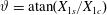 $\unicode[STIX]{x1D717}=\text{atan}(X_{1s}/X_{1c})$
and adding or subtracting the result at
$\unicode[STIX]{x1D717}=\text{atan}(X_{1s}/X_{1c})$
and adding or subtracting the result at
 $\unicode[STIX]{x1D717}=\unicode[STIX]{x03C0}+\text{atan}(X_{1s}/X_{1c})$
, one finds
$\unicode[STIX]{x1D717}=\unicode[STIX]{x03C0}+\text{atan}(X_{1s}/X_{1c})$
, one finds
 $\unicode[STIX]{x2202}t^{(0)}(\unicode[STIX]{x1D717},\unicode[STIX]{x1D711})/\unicode[STIX]{x2202}\unicode[STIX]{x1D717}=0$
.
$\unicode[STIX]{x2202}t^{(0)}(\unicode[STIX]{x1D717},\unicode[STIX]{x1D711})/\unicode[STIX]{x2202}\unicode[STIX]{x1D717}=0$
.
Next, the
 $\boldsymbol{t}$
component of (B 5) implies
$\boldsymbol{t}$
component of (B 5) implies
 $f^{(1)}(\unicode[STIX]{x1D717},\unicode[STIX]{x1D711})=f^{(1)}(\unicode[STIX]{x1D711})$
. The average of (B 5) over
$f^{(1)}(\unicode[STIX]{x1D717},\unicode[STIX]{x1D711})=f^{(1)}(\unicode[STIX]{x1D711})$
. The average of (B 5) over
 $\unicode[STIX]{x1D717}$
then gives
$\unicode[STIX]{x1D717}$
then gives
 $$\begin{eqnarray}\tilde{\boldsymbol{r}}_{0}^{(1)}(\bar{\unicode[STIX]{x1D711}})+f^{(1)}(\unicode[STIX]{x1D711})[1+f^{(0)\prime }(\unicode[STIX]{x1D711})]^{-1}\boldsymbol{t}(\unicode[STIX]{x1D711})[\boldsymbol{r}_{0}^{\prime }(\unicode[STIX]{x1D711})\boldsymbol{\cdot }\boldsymbol{r}_{0}^{\prime }(\unicode[STIX]{x1D711})]^{1/2}=0.\end{eqnarray}$$
The
 $\boldsymbol{n}$
component of (B 5) gives
$\boldsymbol{n}$
component of (B 5) gives
 $$\begin{eqnarray}\left(\begin{array}{@{}c@{}}\tilde{X}_{1s}^{(0)}(\bar{\unicode[STIX]{x1D711}})\\ \tilde{X}_{1c}^{(0)}(\bar{\unicode[STIX]{x1D711}})\end{array}\right)=\left(\begin{array}{@{}cc@{}}\cos (t^{(0)}(\unicode[STIX]{x1D711})) & \sin (t^{(0)}(\unicode[STIX]{x1D711}))\\ -\text{sin}(t^{(0)}(\unicode[STIX]{x1D711})) & \cos (t^{(0)}(\unicode[STIX]{x1D711}))\end{array}\right)\left(\begin{array}{@{}c@{}}X_{1s}(\unicode[STIX]{x1D711})\\ X_{1c}(\unicode[STIX]{x1D711})\end{array}\right),\end{eqnarray}$$
and the
 $\boldsymbol{b}$
component of (B 5) gives the same result but with
$\boldsymbol{b}$
component of (B 5) gives the same result but with
 $X\rightarrow Y$
. Plugging these results into the
$X\rightarrow Y$
. Plugging these results into the
 $O((r/{\mathcal{R}})^{0})$
terms in the tilde version of (A 21),
$O((r/{\mathcal{R}})^{0})$
terms in the tilde version of (A 21),
 $$\begin{eqnarray}\tilde{X}_{1c}^{(0)}(\bar{\unicode[STIX]{x1D711}}){\tilde{Y}}_{1s}^{(0)}(\bar{\unicode[STIX]{x1D711}})-\tilde{X}_{1s}^{(0)}(\bar{\unicode[STIX]{x1D711}}){\tilde{Y}}_{1c}^{(0)}(\bar{\unicode[STIX]{x1D711}})=\frac{s_{G}\bar{B}}{\tilde{B}_{0}^{(0)}(\bar{\unicode[STIX]{x1D711}})},\end{eqnarray}$$
and comparing to the non-tilde version of (A 21), we conclude
 $\tilde{B}_{0}^{(0)}(\bar{\unicode[STIX]{x1D711}})=B_{0}(\unicode[STIX]{x1D711})$
. Applying this result and the derivative of (B 4) in the
$\tilde{B}_{0}^{(0)}(\bar{\unicode[STIX]{x1D711}})=B_{0}(\unicode[STIX]{x1D711})$
. Applying this result and the derivative of (B 4) in the
 $O((r/{\mathcal{R}})^{0})$
tilde version of (A 20),
$O((r/{\mathcal{R}})^{0})$
tilde version of (A 20),
 $$\begin{eqnarray}\tilde{G}_{0}^{(0)}=s_{G}\tilde{B}_{0}^{(0)}(\bar{\unicode[STIX]{x1D711}})[\tilde{\boldsymbol{r}}_{0}^{(0)\prime }(\bar{\unicode[STIX]{x1D711}})\boldsymbol{\cdot }\tilde{\boldsymbol{r}}_{0}^{(0)\prime }(\bar{\unicode[STIX]{x1D711}})]^{1/2},\end{eqnarray}$$
we obtain
 $\tilde{G}_{0}^{(0)}=G_{0}/[1+f^{(0)\prime }(\unicode[STIX]{x1D711})]$
, which implies
$\tilde{G}_{0}^{(0)}=G_{0}/[1+f^{(0)\prime }(\unicode[STIX]{x1D711})]$
, which implies
 $f^{(0)\prime }(\unicode[STIX]{x1D711})=0$
. From (B 3), then
$f^{(0)\prime }(\unicode[STIX]{x1D711})=0$
. From (B 3), then
 $f^{(0)}=0$
, so
$f^{(0)}=0$
, so
 $\tilde{G}_{0}^{(0)}=G_{0}$
. Since
$\tilde{G}_{0}^{(0)}=G_{0}$
. Since
 $\bar{\unicode[STIX]{x1D711}}=\unicode[STIX]{x1D711}$
, we can simplify notation in the remainder of this appendix: functions of a single argument can be assumed to have argument
$\bar{\unicode[STIX]{x1D711}}=\unicode[STIX]{x1D711}$
, we can simplify notation in the remainder of this appendix: functions of a single argument can be assumed to have argument
 $\unicode[STIX]{x1D711}$
.
$\unicode[STIX]{x1D711}$
.
Next,
 $t^{(0)}$
can be constrained using the
$t^{(0)}$
can be constrained using the
 $O((r/{\mathcal{R}})^{0})$
terms in the tilde version of (A 23),
$O((r/{\mathcal{R}})^{0})$
terms in the tilde version of (A 23),
 $$\begin{eqnarray}\displaystyle & & \displaystyle (\tilde{\unicode[STIX]{x1D704}}_{0}^{(0)}-N)[\tilde{X}_{1s}^{(0)2}+\tilde{X}_{1c}^{(0)2}+{\tilde{Y}}_{1s}^{(0)2}+{\tilde{Y}}_{1c}^{(0)2}]\nonumber\\ \displaystyle & & \displaystyle \quad =\tilde{X}_{1c}^{(0)}\tilde{X}_{1s}^{(0)\prime }-\tilde{X}_{1s}^{(0)}\tilde{X}_{1c}^{(0)\prime }+{\tilde{Y}}_{1c}^{(0)}{\tilde{Y}}_{1s}^{(0)\prime }-{\tilde{Y}}_{1s}^{(0)}{\tilde{Y}}_{1c}^{(0)\prime }+2\left(\frac{I_{2}}{\bar{B}}-\tilde{\unicode[STIX]{x1D70F}}^{(0)}\right)\frac{G_{0}\bar{B}}{B_{0}^{2}}.\end{eqnarray}$$
Substituting (B 7) (and its
 $X\rightarrow Y$
equivalent) and subtracting the non-tilde version of (A 23), one finds
$X\rightarrow Y$
equivalent) and subtracting the non-tilde version of (A 23), one finds
 $\tilde{\unicode[STIX]{x1D704}}_{0}^{(0)}-\unicode[STIX]{x1D704}_{0}=t^{(0)\prime }(\unicode[STIX]{x1D711})$
, which implies
$\tilde{\unicode[STIX]{x1D704}}_{0}^{(0)}-\unicode[STIX]{x1D704}_{0}=t^{(0)\prime }(\unicode[STIX]{x1D711})$
, which implies
 $\tilde{\unicode[STIX]{x1D704}}_{0}^{(0)}=\unicode[STIX]{x1D704}_{0}$
and
$\tilde{\unicode[STIX]{x1D704}}_{0}^{(0)}=\unicode[STIX]{x1D704}_{0}$
and
 $t^{(0)\prime }(\unicode[STIX]{x1D711})=0$
. From (B 3), then
$t^{(0)\prime }(\unicode[STIX]{x1D711})=0$
. From (B 3), then
 $t^{(0)}=0$
. Then (B 7) gives
$t^{(0)}=0$
. Then (B 7) gives
 $$\begin{eqnarray}\tilde{X}_{1s}^{(0)}=X_{1s},\quad \tilde{X}_{1c}^{(0)}=X_{1c},\quad {\tilde{Y}}_{1s}^{(0)}=Y_{1s},\quad {\tilde{Y}}_{1c}^{(0)}=Y_{1c}.\end{eqnarray}$$
The
 $O((r/{\mathcal{R}})^{0})$
terms in the tilde version of (A 22) then give
$O((r/{\mathcal{R}})^{0})$
terms in the tilde version of (A 22) then give
 $\tilde{B}_{1}^{(0)}(\unicode[STIX]{x1D711})=B_{1}(\unicode[STIX]{x1D711})$
.
$\tilde{B}_{1}^{(0)}(\unicode[STIX]{x1D711})=B_{1}(\unicode[STIX]{x1D711})$
.
We proceed to the
 $O((r/{\mathcal{R}})^{2})$
terms in (3.8),
$O((r/{\mathcal{R}})^{2})$
terms in (3.8),
 $$\begin{eqnarray}\displaystyle & & \displaystyle X_{2}(\unicode[STIX]{x1D717},\unicode[STIX]{x1D711})\boldsymbol{n}+Y_{2}(\unicode[STIX]{x1D717},\unicode[STIX]{x1D711})\boldsymbol{b}+Z_{2}(\unicode[STIX]{x1D717},\unicode[STIX]{x1D711})\boldsymbol{t}\nonumber\\ \displaystyle & & \displaystyle \quad =\tilde{\boldsymbol{r}}_{0}^{(2)}+f^{(1)}\tilde{\boldsymbol{r}}_{0}^{(1)\prime }+f^{(2)}(\unicode[STIX]{x1D717},\unicode[STIX]{x1D711})\boldsymbol{r}_{0}^{\prime }+\frac{1}{2}f^{(1)2}\boldsymbol{r}_{0}^{\prime \prime }\nonumber\\ \displaystyle & & \displaystyle \qquad +\,\tilde{X}_{2}^{(0)}(\unicode[STIX]{x1D717},\unicode[STIX]{x1D711})\boldsymbol{n}+\tilde{X}_{1}^{(1)}(\unicode[STIX]{x1D717},\unicode[STIX]{x1D711})\boldsymbol{n}+X_{1}(\unicode[STIX]{x1D717},\unicode[STIX]{x1D711})\tilde{\boldsymbol{n}}^{(1)}+f^{(1)}X_{1}(\unicode[STIX]{x1D717},\unicode[STIX]{x1D711})\boldsymbol{n}^{\prime }\nonumber\\ \displaystyle & & \displaystyle \qquad +\,t^{(1)}(\unicode[STIX]{x1D717},\unicode[STIX]{x1D711})\boldsymbol{n}\unicode[STIX]{x2202}_{1}X_{1}(\unicode[STIX]{x1D717},\unicode[STIX]{x1D711})+f^{(1)}\boldsymbol{n}\unicode[STIX]{x2202}_{2}X_{1}(\unicode[STIX]{x1D717},\unicode[STIX]{x1D711})\nonumber\\ \displaystyle & & \displaystyle \qquad +\,{\tilde{Y}}_{2}^{(0)}(\unicode[STIX]{x1D717},\unicode[STIX]{x1D711})\boldsymbol{b}+{\tilde{Y}}_{1}^{(1)}(\unicode[STIX]{x1D717},\unicode[STIX]{x1D711})\boldsymbol{b}+Y_{1}(\unicode[STIX]{x1D717},\unicode[STIX]{x1D711})\tilde{\boldsymbol{b}}^{(1)}+f^{(1)}Y_{1}(\unicode[STIX]{x1D717},\unicode[STIX]{x1D711})\boldsymbol{b}^{\prime }\nonumber\\ \displaystyle & & \displaystyle \qquad +\,t^{(1)}(\unicode[STIX]{x1D717},\unicode[STIX]{x1D711})\boldsymbol{b}\unicode[STIX]{x2202}_{1}Y_{1}(\unicode[STIX]{x1D717},\unicode[STIX]{x1D711})+f^{(1)}\boldsymbol{b}\unicode[STIX]{x2202}_{2}Y_{1}(\unicode[STIX]{x1D717},\unicode[STIX]{x1D711})+\tilde{Z}_{2}^{(0)}(\unicode[STIX]{x1D717},\unicode[STIX]{x1D711})\boldsymbol{t},\end{eqnarray}$$
where
 $\unicode[STIX]{x2202}_{1}$
and
$\unicode[STIX]{x2202}_{1}$
and
 $\unicode[STIX]{x2202}_{2}$
indicate partial derivatives with respect to the first or second argument. (If the construction is done only through
$\unicode[STIX]{x2202}_{2}$
indicate partial derivatives with respect to the first or second argument. (If the construction is done only through
 $O((r/{\mathcal{R}})^{1})$
, the left-hand side is zero.) Applying
$O((r/{\mathcal{R}})^{1})$
, the left-hand side is zero.) Applying
 $\unicode[STIX]{x03C0}^{-1}\int _{0}^{2\unicode[STIX]{x03C0}}\text{d}\unicode[STIX]{x1D717}(\sin \unicode[STIX]{x1D717})(\cdots \,)$
and
$\unicode[STIX]{x03C0}^{-1}\int _{0}^{2\unicode[STIX]{x03C0}}\text{d}\unicode[STIX]{x1D717}(\sin \unicode[STIX]{x1D717})(\cdots \,)$
and
 $\unicode[STIX]{x03C0}^{-1}\int _{0}^{2\unicode[STIX]{x03C0}}\text{d}\unicode[STIX]{x1D717}(\cos \unicode[STIX]{x1D717})(\cdots \,)$
to the
$\unicode[STIX]{x03C0}^{-1}\int _{0}^{2\unicode[STIX]{x03C0}}\text{d}\unicode[STIX]{x1D717}(\cos \unicode[STIX]{x1D717})(\cdots \,)$
to the
 $\boldsymbol{n}$
component,
$\boldsymbol{n}$
component,
 $$\begin{eqnarray}\displaystyle & \displaystyle \tilde{X}_{1s}^{(1)}=-X_{1s}t_{sc}^{(1)}+X_{1c}t_{ss}^{(1)}-f^{(1)}X_{1s}^{\prime }-Y_{1s}\boldsymbol{n}\boldsymbol{\cdot }\tilde{\boldsymbol{b}}^{(1)}-f^{(1)}Y_{1s}\boldsymbol{n}\boldsymbol{\cdot }\boldsymbol{b}^{\prime }, & \displaystyle\end{eqnarray}$$
 $$\begin{eqnarray}\displaystyle & \displaystyle \tilde{X}_{1c}^{(1)}=-X_{1s}t_{cc}^{(1)}+X_{1c}t_{sc}^{(1)}-f^{(1)}X_{1c}^{\prime }-Y_{1c}\boldsymbol{n}\boldsymbol{\cdot }\tilde{\boldsymbol{b}}^{(1)}-f^{(1)}Y_{1c}\boldsymbol{n}\boldsymbol{\cdot }\boldsymbol{b}^{\prime }, & \displaystyle\end{eqnarray}$$
where
 $$\begin{eqnarray}\displaystyle & \displaystyle t_{ss}^{(1)}(\unicode[STIX]{x1D711})=\unicode[STIX]{x03C0}^{-1}\int _{0}^{2\unicode[STIX]{x03C0}}\text{d}\unicode[STIX]{x1D717}t^{(1)}(\unicode[STIX]{x1D717},\unicode[STIX]{x1D711})\sin ^{2}\unicode[STIX]{x1D717}, & \displaystyle\end{eqnarray}$$
 $$\begin{eqnarray}\displaystyle & \displaystyle t_{sc}^{(1)}(\unicode[STIX]{x1D711})=\unicode[STIX]{x03C0}^{-1}\int _{0}^{2\unicode[STIX]{x03C0}}\text{d}\unicode[STIX]{x1D717}t^{(1)}(\unicode[STIX]{x1D717},\unicode[STIX]{x1D711})\sin \unicode[STIX]{x1D717}\cos \unicode[STIX]{x1D717}, & \displaystyle\end{eqnarray}$$
 $$\begin{eqnarray}\displaystyle & \displaystyle t_{cc}^{(1)}(\unicode[STIX]{x1D711})=\unicode[STIX]{x03C0}^{-1}\int _{0}^{2\unicode[STIX]{x03C0}}\text{d}\unicode[STIX]{x1D717}t^{(1)}(\unicode[STIX]{x1D717},\unicode[STIX]{x1D711})\cos ^{2}\unicode[STIX]{x1D717}. & \displaystyle\end{eqnarray}$$
We have used
 $\boldsymbol{n}\boldsymbol{\cdot }\tilde{\boldsymbol{n}}^{(1)}=0$
since this is the
$\boldsymbol{n}\boldsymbol{\cdot }\tilde{\boldsymbol{n}}^{(1)}=0$
since this is the
 $O(r/{\mathcal{R}})$
term in
$O(r/{\mathcal{R}})$
term in
 $|\tilde{\boldsymbol{n}}|=1$
. Similarly, from the
$|\tilde{\boldsymbol{n}}|=1$
. Similarly, from the
 $\boldsymbol{b}$
component of (B 12),
$\boldsymbol{b}$
component of (B 12),
 $$\begin{eqnarray}\displaystyle & \displaystyle {\tilde{Y}}_{1s}^{(1)}=-Y_{1s}t_{sc}^{(1)}+Y_{1c}t_{ss}^{(1)}-f^{(1)}Y_{1s}^{\prime }-X_{1s}\boldsymbol{b}\boldsymbol{\cdot }\tilde{\boldsymbol{n}}^{(1)}-f^{(1)}X_{1s}\boldsymbol{b}\boldsymbol{\cdot }\boldsymbol{n}^{\prime }, & \displaystyle\end{eqnarray}$$
 $$\begin{eqnarray}\displaystyle & \displaystyle {\tilde{Y}}_{1c}^{(1)}=-Y_{1s}t_{cc}^{(1)}+Y_{1c}t_{sc}^{(1)}-f^{(1)}Y_{1c}^{\prime }-X_{1c}\boldsymbol{b}\boldsymbol{\cdot }\tilde{\boldsymbol{n}}^{(1)}-f^{(1)}X_{1c}\boldsymbol{b}\boldsymbol{\cdot }\boldsymbol{n}^{\prime }. & \displaystyle\end{eqnarray}$$
Equations (B 13)–(B 19) are substituted into the
 $O(r/{\mathcal{R}})$
terms in the tilde version of (A 21),
$O(r/{\mathcal{R}})$
terms in the tilde version of (A 21),
 $$\begin{eqnarray}X_{1c}{\tilde{Y}}_{1s}^{(1)}+\tilde{X}_{1c}^{(1)}Y_{1s}-X_{1s}{\tilde{Y}}_{1c}^{(1)}-\tilde{X}_{1s}^{(1)}Y_{1c}=-\frac{s_{G}\bar{B}\tilde{B}_{0}^{(1)}}{B_{0}^{2}},\end{eqnarray}$$
which after many cancellations gives
 $$\begin{eqnarray}s_{G}\bar{B}\tilde{B}_{0}^{(1)}/B_{0}^{2}=f^{(1)}[X_{1c}Y_{1s}-X_{1s}Y_{1c}]^{\prime }.\end{eqnarray}$$
From (A 21),
 $$\begin{eqnarray}\tilde{B}_{0}^{(1)}=-f^{(1)}B_{0}^{\prime }.\end{eqnarray}$$
To determine
 $f^{(1)}$
, this result and (B 6) are substituted into the
$f^{(1)}$
, this result and (B 6) are substituted into the
 $O((r/{\mathcal{R}})^{1})$
terms of the tilde version of (A 20):
$O((r/{\mathcal{R}})^{1})$
terms of the tilde version of (A 20):
 $$\begin{eqnarray}\tilde{G}_{0}^{(1)}=s_{G}\tilde{B}_{0}^{(1)}\ell ^{\prime }+\frac{s_{G}B_{0}}{\ell ^{\prime }}\boldsymbol{r}_{0}^{\prime }\boldsymbol{\cdot }\tilde{\boldsymbol{r}}_{0}^{(1)\prime }.\end{eqnarray}$$
As a result we find
 $\tilde{G}_{0}^{(1)}=-f^{(1)\prime }(\unicode[STIX]{x1D711})G_{0}$
. Since
$\tilde{G}_{0}^{(1)}=-f^{(1)\prime }(\unicode[STIX]{x1D711})G_{0}$
. Since
 $f^{(1)}(\unicode[STIX]{x1D711})$
is single-valued,
$f^{(1)}(\unicode[STIX]{x1D711})$
is single-valued,
 $\tilde{G}_{0}^{(1)}=0$
and
$\tilde{G}_{0}^{(1)}=0$
and
 $f^{(1)\prime }(\unicode[STIX]{x1D711})=0$
. Then by (B 3),
$f^{(1)\prime }(\unicode[STIX]{x1D711})=0$
. Then by (B 3),
 $f^{(1)}=0$
. Then (B 22) gives
$f^{(1)}=0$
. Then (B 22) gives
 $\tilde{B}_{0}^{(1)}(\unicode[STIX]{x1D711})=0$
.
$\tilde{B}_{0}^{(1)}(\unicode[STIX]{x1D711})=0$
.
At this point, we have proved the first set of assertions following (3.9): when a finite
 $r=a$
is plugged into a solution of the
$r=a$
is plugged into a solution of the
 $O((r/{\mathcal{R}})^{1})$
Garren–Boozer equations, the real finite-minor-radius MHD equilibrium inside the constructed boundary has the desired magnetic field as a function of Boozer coordinates through
$O((r/{\mathcal{R}})^{1})$
Garren–Boozer equations, the real finite-minor-radius MHD equilibrium inside the constructed boundary has the desired magnetic field as a function of Boozer coordinates through
 $O(r/{\mathcal{R}})$
.
$O(r/{\mathcal{R}})$
.
B.3 The
$O((r/{\mathcal{R}})^{2})$
construction

We now proceed to evaluate
 $\tilde{B}(a,r,\tilde{\unicode[STIX]{x1D717}},\tilde{\unicode[STIX]{x1D711}})$
through
$\tilde{B}(a,r,\tilde{\unicode[STIX]{x1D717}},\tilde{\unicode[STIX]{x1D711}})$
through
 $O((r/{\mathcal{R}})^{2})$
. First,
$O((r/{\mathcal{R}})^{2})$
. First,
 $f^{(1)}=0$
and (B 6) imply
$f^{(1)}=0$
and (B 6) imply
 $\tilde{\boldsymbol{r}}_{0}^{(1)}=0$
. The
$\tilde{\boldsymbol{r}}_{0}^{(1)}=0$
. The
 $O(r/{\mathcal{R}})$
terms in the Frenet relations for the tilde configuration then imply
$O(r/{\mathcal{R}})$
terms in the Frenet relations for the tilde configuration then imply
 $\tilde{\boldsymbol{t}}^{(1)}=\tilde{\boldsymbol{n}}^{(1)}=\tilde{\boldsymbol{b}}^{(1)}=\unicode[STIX]{x1D705}^{(1)}=\unicode[STIX]{x1D70F}^{(1)}=0$
.
$\tilde{\boldsymbol{t}}^{(1)}=\tilde{\boldsymbol{n}}^{(1)}=\tilde{\boldsymbol{b}}^{(1)}=\unicode[STIX]{x1D705}^{(1)}=\unicode[STIX]{x1D70F}^{(1)}=0$
.
At this point, we assume the construction is done through at least
 $O((r/{\mathcal{R}})^{2})$
. Since
$O((r/{\mathcal{R}})^{2})$
. Since
 $Z_{2}$
is given by a unique function of
$Z_{2}$
is given by a unique function of
 $X_{1}$
and
$X_{1}$
and
 $Y_{1}$
by (A 27)–(A 29), then
$Y_{1}$
by (A 27)–(A 29), then
 $\tilde{Z}_{2}^{(0)}(\unicode[STIX]{x1D717},\unicode[STIX]{x1D711})=Z_{2}(\unicode[STIX]{x1D717},\unicode[STIX]{x1D711})$
. Then the
$\tilde{Z}_{2}^{(0)}(\unicode[STIX]{x1D717},\unicode[STIX]{x1D711})=Z_{2}(\unicode[STIX]{x1D717},\unicode[STIX]{x1D711})$
. Then the
 $\boldsymbol{t}$
component of (B 12) implies
$\boldsymbol{t}$
component of (B 12) implies
 $f^{(2)}(\unicode[STIX]{x1D717},\unicode[STIX]{x1D711})=f^{(2)}(\unicode[STIX]{x1D711})$
.
$f^{(2)}(\unicode[STIX]{x1D717},\unicode[STIX]{x1D711})=f^{(2)}(\unicode[STIX]{x1D711})$
.
The terms remaining in the
 $\boldsymbol{n}$
component of (B 12) are
$\boldsymbol{n}$
component of (B 12) are
 $$\begin{eqnarray}X_{2}(\unicode[STIX]{x1D717},\unicode[STIX]{x1D711})=\boldsymbol{n}\boldsymbol{\cdot }\tilde{\boldsymbol{r}}_{0}^{(2)}+\tilde{X}_{2}^{(0)}(\unicode[STIX]{x1D717},\unicode[STIX]{x1D711})+\tilde{X}_{1}^{(1)}(\unicode[STIX]{x1D717},\unicode[STIX]{x1D711})+t^{(1)}(\unicode[STIX]{x1D717},\unicode[STIX]{x1D711})[X_{1s}\cos \unicode[STIX]{x1D717}-X_{1c}\sin \unicode[STIX]{x1D717}].\end{eqnarray}$$
We are free to define
 $$\begin{eqnarray}\displaystyle \bar{t}(\unicode[STIX]{x1D717},\unicode[STIX]{x1D711}) & = & \displaystyle t^{(1)}(\unicode[STIX]{x1D717},\unicode[STIX]{x1D711})-\frac{2}{X_{1s}^{2}+X_{1c}^{2}}[(X_{2s}-\tilde{X}_{2s}^{(0)})X_{1s}+(X_{2c}-\tilde{X}_{2c}^{(0)})X_{1c}]\sin \unicode[STIX]{x1D717}\nonumber\\ \displaystyle & & \displaystyle -\,\frac{2}{X_{1s}^{2}+X_{1c}^{2}}[(X_{2c}-\tilde{X}_{2c}^{(0)})X_{1s}-(X_{2s}-\tilde{X}_{2s}^{(0)})X_{1c}]\cos \unicode[STIX]{x1D717}.\end{eqnarray}$$
Then (B 24) can be written
 $$\begin{eqnarray}0=C(\unicode[STIX]{x1D711})+\tilde{X}_{1s}^{(1)}\sin \unicode[STIX]{x1D717}+\tilde{X}_{1c}^{(1)}\cos \unicode[STIX]{x1D717}+\bar{t}(\unicode[STIX]{x1D717},\unicode[STIX]{x1D711})[X_{1s}\cos \unicode[STIX]{x1D717}-X_{1c}\sin \unicode[STIX]{x1D717}]\end{eqnarray}$$
for a
 $\unicode[STIX]{x1D717}$
-independent function
$\unicode[STIX]{x1D717}$
-independent function
 $C(\unicode[STIX]{x1D711})$
. Evaluating (B 26) at
$C(\unicode[STIX]{x1D711})$
. Evaluating (B 26) at
 $\unicode[STIX]{x1D717}=\text{atan}(X_{1s}/X_{1c})$
, and adding or subtracting (B 26) at
$\unicode[STIX]{x1D717}=\text{atan}(X_{1s}/X_{1c})$
, and adding or subtracting (B 26) at
 $\unicode[STIX]{x1D717}=\unicode[STIX]{x03C0}+\text{atan}(X_{1s}/X_{1c})$
, we find
$\unicode[STIX]{x1D717}=\unicode[STIX]{x03C0}+\text{atan}(X_{1s}/X_{1c})$
, we find
 $C=0$
and
$C=0$
and
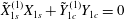 $\tilde{X}_{1s}^{(1)}X_{1s}+{\tilde{Y}}_{1c}^{(1)}Y_{1c}=0$
. Then (B 26) implies
$\tilde{X}_{1s}^{(1)}X_{1s}+{\tilde{Y}}_{1c}^{(1)}Y_{1c}=0$
. Then (B 26) implies
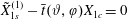 $\tilde{X}_{1s}^{(1)}-\bar{t}(\unicode[STIX]{x1D717},\unicode[STIX]{x1D711})X_{1c}=0$
, so
$\tilde{X}_{1s}^{(1)}-\bar{t}(\unicode[STIX]{x1D717},\unicode[STIX]{x1D711})X_{1c}=0$
, so
 $\bar{t}(\unicode[STIX]{x1D717},\unicode[STIX]{x1D711})=\bar{t}(\unicode[STIX]{x1D711})$
.
$\bar{t}(\unicode[STIX]{x1D717},\unicode[STIX]{x1D711})=\bar{t}(\unicode[STIX]{x1D711})$
.
Repeating the analysis from (B 24) with the
 $\boldsymbol{b}$
component of (B 12), we find (B 25) with
$\boldsymbol{b}$
component of (B 12), we find (B 25) with
 $X\rightarrow Y$
. Comparing the
$X\rightarrow Y$
. Comparing the
 $\sin \unicode[STIX]{x1D717}$
and
$\sin \unicode[STIX]{x1D717}$
and
 $\cos \unicode[STIX]{x1D717}$
modes of this result with those of (B 25), then
$\cos \unicode[STIX]{x1D717}$
modes of this result with those of (B 25), then
 $$\begin{eqnarray}\displaystyle & \displaystyle \frac{\unicode[STIX]{x1D709}_{s}X_{1s}+\unicode[STIX]{x1D709}_{c}X_{1c}}{X_{1s}^{2}+X_{1c}^{2}}=\frac{\unicode[STIX]{x1D6FE}_{s}Y_{1s}+\unicode[STIX]{x1D6FE}_{c}Y_{1c}}{Y_{1s}^{2}+Y_{1c}^{2}}, & \displaystyle\end{eqnarray}$$
 $$\begin{eqnarray}\displaystyle & \displaystyle \frac{\unicode[STIX]{x1D709}_{c}X_{1s}-\unicode[STIX]{x1D709}_{s}X_{1c}}{X_{1s}^{2}+X_{1c}^{2}}=\frac{\unicode[STIX]{x1D6FE}_{c}Y_{1s}-\unicode[STIX]{x1D6FE}_{s}Y_{1c}}{Y_{1s}^{2}+Y_{1c}^{2}}, & \displaystyle\end{eqnarray}$$
where
 $\unicode[STIX]{x1D709}_{s}=X_{2s}-\tilde{X}_{2s}^{(0)}$
,
$\unicode[STIX]{x1D709}_{s}=X_{2s}-\tilde{X}_{2s}^{(0)}$
,
 $\unicode[STIX]{x1D709}_{c}=X_{2c}-\tilde{X}_{2c}^{(0)}$
,
$\unicode[STIX]{x1D709}_{c}=X_{2c}-\tilde{X}_{2c}^{(0)}$
,
 $\unicode[STIX]{x1D6FE}_{s}=Y_{2s}-{\tilde{Y}}_{2s}^{(0)}$
and
$\unicode[STIX]{x1D6FE}_{s}=Y_{2s}-{\tilde{Y}}_{2s}^{(0)}$
and
 $\unicode[STIX]{x1D6FE}_{c}=Y_{2c}-{\tilde{Y}}_{2c}^{(0)}$
. We obtain four other linear homogeneous equations relating
$\unicode[STIX]{x1D6FE}_{c}=Y_{2c}-{\tilde{Y}}_{2c}^{(0)}$
. We obtain four other linear homogeneous equations relating
 $\{\unicode[STIX]{x1D709}_{s},\unicode[STIX]{x1D709}_{c},\unicode[STIX]{x1D6FE}_{s},\unicode[STIX]{x1D6FE}_{c}\}$
by taking the non-tilde versions of (A 41)–(A 42) and (A 32)–(A 33) and subtracting the
$\{\unicode[STIX]{x1D709}_{s},\unicode[STIX]{x1D709}_{c},\unicode[STIX]{x1D6FE}_{s},\unicode[STIX]{x1D6FE}_{c}\}$
by taking the non-tilde versions of (A 41)–(A 42) and (A 32)–(A 33) and subtracting the
 $O((r/{\mathcal{R}})^{0})$
tilde versions. These four equations also involve
$O((r/{\mathcal{R}})^{0})$
tilde versions. These four equations also involve
 $\unicode[STIX]{x1D709}_{0}=X_{20}-\tilde{X}_{20}^{(0)}$
and
$\unicode[STIX]{x1D709}_{0}=X_{20}-\tilde{X}_{20}^{(0)}$
and
 $\unicode[STIX]{x1D6FE}_{0}=Y_{20}-{\tilde{Y}}_{20}^{(0)}$
. We thus have six linear homogeneous equations relating the six unknowns
$\unicode[STIX]{x1D6FE}_{0}=Y_{20}-{\tilde{Y}}_{20}^{(0)}$
. We thus have six linear homogeneous equations relating the six unknowns
 $\{\unicode[STIX]{x1D709}_{0},\unicode[STIX]{x1D709}_{s},\unicode[STIX]{x1D709}_{c},\unicode[STIX]{x1D6FE}_{0},\unicode[STIX]{x1D6FE}_{s},\unicode[STIX]{x1D6FE}_{c}\}$
. A valid solution is the one in which all six quantities vanish. The six equations are generally linearly independent, and so this is the unique solution. Hence,
$\{\unicode[STIX]{x1D709}_{0},\unicode[STIX]{x1D709}_{s},\unicode[STIX]{x1D709}_{c},\unicode[STIX]{x1D6FE}_{0},\unicode[STIX]{x1D6FE}_{s},\unicode[STIX]{x1D6FE}_{c}\}$
. A valid solution is the one in which all six quantities vanish. The six equations are generally linearly independent, and so this is the unique solution. Hence,
 $\tilde{X}_{2}^{(0)}(\unicode[STIX]{x1D717},\unicode[STIX]{x1D711})=X_{2}(\unicode[STIX]{x1D717},\unicode[STIX]{x1D711})$
and
$\tilde{X}_{2}^{(0)}(\unicode[STIX]{x1D717},\unicode[STIX]{x1D711})=X_{2}(\unicode[STIX]{x1D717},\unicode[STIX]{x1D711})$
and
 ${\tilde{Y}}_{2}^{(0)}(\unicode[STIX]{x1D717},\unicode[STIX]{x1D711})=Y_{2}(\unicode[STIX]{x1D717},\unicode[STIX]{x1D711})$
. Comparing the non-tilde and the
${\tilde{Y}}_{2}^{(0)}(\unicode[STIX]{x1D717},\unicode[STIX]{x1D711})=Y_{2}(\unicode[STIX]{x1D717},\unicode[STIX]{x1D711})$
. Comparing the non-tilde and the
 $O((r/{\mathcal{R}})^{0})$
tilde versions of (A 34)–(A 36), we conclude
$O((r/{\mathcal{R}})^{0})$
tilde versions of (A 34)–(A 36), we conclude
 $\tilde{B}_{2}^{(0)}(\unicode[STIX]{x1D717},\unicode[STIX]{x1D711})=B_{2}(\unicode[STIX]{x1D717},\unicode[STIX]{x1D711})$
. This completes the evaluation of one more term in (3.9).
$\tilde{B}_{2}^{(0)}(\unicode[STIX]{x1D717},\unicode[STIX]{x1D711})=B_{2}(\unicode[STIX]{x1D717},\unicode[STIX]{x1D711})$
. This completes the evaluation of one more term in (3.9).
Knowing now that
 $t^{(1)}(\unicode[STIX]{x1D717},\unicode[STIX]{x1D711})=t^{(1)}(\unicode[STIX]{x1D711})$
,
$t^{(1)}(\unicode[STIX]{x1D717},\unicode[STIX]{x1D711})=t^{(1)}(\unicode[STIX]{x1D711})$
,
 $f^{(1)}=0$
,
$f^{(1)}=0$
,
 $\tilde{\boldsymbol{n}}^{(1)}=0$
, and
$\tilde{\boldsymbol{n}}^{(1)}=0$
, and
 $\tilde{\boldsymbol{b}}^{(1)}=0$
, we return to (B 13)–(B 19), which become
$\tilde{\boldsymbol{b}}^{(1)}=0$
, we return to (B 13)–(B 19), which become
 $$\begin{eqnarray}\left.\begin{array}{@{}c@{}}\tilde{X}_{1s}^{(1)}=t^{(1)}X_{1c},\quad \tilde{X}_{1c}^{(1)}=-t^{(1)}X_{1s},\\ {\tilde{Y}}_{1s}^{(1)}=t^{(1)}Y_{1c},\quad {\tilde{Y}}_{1c}^{(1)}=-t^{(1)}Y_{1s}.\end{array}\right\}\end{eqnarray}$$
These expressions are substituted into the
 $O(r/{\mathcal{R}})$
terms in the tilde version of (A 23),
$O(r/{\mathcal{R}})$
terms in the tilde version of (A 23),
 $$\begin{eqnarray}\displaystyle & & \displaystyle \tilde{\unicode[STIX]{x1D704}}_{0}^{(1)}[X_{1s}^{2}+X_{1c}^{2}+Y_{1s}^{2}+Y_{1c}^{2}]+2\unicode[STIX]{x1D704}_{0}[X_{1s}\tilde{X}_{1s}^{(1)}+X_{1c}\tilde{X}_{1c}^{(1)}+Y_{1s}{\tilde{Y}}_{1s}^{(1)}+Y_{1c}{\tilde{Y}}_{1c}^{(1)}]\nonumber\\ \displaystyle & & \displaystyle \quad =X_{1c}\tilde{X}_{1s}^{(1)\prime }-X_{1s}\tilde{X}_{1c}^{(1)\prime }+Y_{1c}{\tilde{Y}}_{1s}^{(1)\prime }-Y_{1s}{\tilde{Y}}_{1c}^{(1)\prime }\nonumber\\ \displaystyle & & \displaystyle \qquad +\,\tilde{X}_{1c}^{(1)}X_{1s}^{\prime }-\tilde{X}_{1s}^{(1)}X_{1c}^{\prime }+{\tilde{Y}}_{1c}^{(1)}Y_{1s}^{\prime }-{\tilde{Y}}_{1s}^{(1)}Y_{1c}^{\prime }.\end{eqnarray}$$
The result is
 $\tilde{\unicode[STIX]{x1D704}}_{0}^{(1)}=t^{(1)\prime }(\unicode[STIX]{x1D711})$
, implying
$\tilde{\unicode[STIX]{x1D704}}_{0}^{(1)}=t^{(1)\prime }(\unicode[STIX]{x1D711})$
, implying
 $\tilde{\unicode[STIX]{x1D704}}_{0}^{(1)}=0$
and
$\tilde{\unicode[STIX]{x1D704}}_{0}^{(1)}=0$
and
 $t^{(1)}(\unicode[STIX]{x1D711})=\text{const}$
. From (B 3), then,
$t^{(1)}(\unicode[STIX]{x1D711})=\text{const}$
. From (B 3), then,
 $t^{(1)}=0$
, so
$t^{(1)}=0$
, so
 $\tilde{X}_{1s}^{(1)}=\tilde{X}_{1c}^{(1)}={\tilde{Y}}_{1s}^{(1)}={\tilde{Y}}_{1c}^{(1)}=0$
. The
$\tilde{X}_{1s}^{(1)}=\tilde{X}_{1c}^{(1)}={\tilde{Y}}_{1s}^{(1)}={\tilde{Y}}_{1c}^{(1)}=0$
. The
 $O(r/{\mathcal{R}})$
terms in (A 22) can now be evaluated to give one more term we need in (3.9):
$O(r/{\mathcal{R}})$
terms in (A 22) can now be evaluated to give one more term we need in (3.9):
 $\tilde{B}_{1}^{(1)}(\unicode[STIX]{x1D717},\unicode[STIX]{x1D711})=0$
. The only remaining terms in (B 12) give
$\tilde{B}_{1}^{(1)}(\unicode[STIX]{x1D717},\unicode[STIX]{x1D711})=0$
. The only remaining terms in (B 12) give
 $$\begin{eqnarray}\tilde{\boldsymbol{r}}_{0}^{(2)}=-f^{(2)}\boldsymbol{r}_{0}^{\prime }.\end{eqnarray}$$
We proceed to the
 $O((r/{\mathcal{R}})^{3})$
terms in (3.8),
$O((r/{\mathcal{R}})^{3})$
terms in (3.8),
 $$\begin{eqnarray}\displaystyle & & \displaystyle X_{3}(\unicode[STIX]{x1D717},\unicode[STIX]{x1D711})\boldsymbol{n}+Y_{3}(\unicode[STIX]{x1D717},\unicode[STIX]{x1D711})\boldsymbol{b}+Z_{3}(\unicode[STIX]{x1D717},\unicode[STIX]{x1D711})\boldsymbol{t}=\tilde{\boldsymbol{r}}_{0}^{(3)}+f^{(3)}(\unicode[STIX]{x1D717},\unicode[STIX]{x1D711})\boldsymbol{r}_{0}^{\prime }+\boldsymbol{t}\tilde{Z}_{3}^{(0)}(\unicode[STIX]{x1D717},\unicode[STIX]{x1D711})+\boldsymbol{t}\tilde{Z}_{2}^{(1)}(\unicode[STIX]{x1D717},\unicode[STIX]{x1D711})\nonumber\\ \displaystyle & & \displaystyle \quad +\,\boldsymbol{n}\tilde{X}_{3}^{(0)}(\unicode[STIX]{x1D717},\unicode[STIX]{x1D711})+\tilde{\boldsymbol{n}}^{(2)}X_{1}(\unicode[STIX]{x1D717},\unicode[STIX]{x1D711})+\boldsymbol{n}\tilde{X}_{1}^{(2)}(\unicode[STIX]{x1D717},\unicode[STIX]{x1D711})+\boldsymbol{n}\tilde{X}_{2}^{(1)}(\unicode[STIX]{x1D717},\unicode[STIX]{x1D711})\nonumber\\ \displaystyle & & \displaystyle \quad +\,\boldsymbol{b}{\tilde{Y}}_{3}^{(0)}(\unicode[STIX]{x1D717},\unicode[STIX]{x1D711})+\tilde{\boldsymbol{b}}^{(2)}Y_{1}(\unicode[STIX]{x1D717},\unicode[STIX]{x1D711})+\boldsymbol{b}{\tilde{Y}}_{1}^{(2)}(\unicode[STIX]{x1D717},\unicode[STIX]{x1D711})+\boldsymbol{b}{\tilde{Y}}_{2}^{(1)}(\unicode[STIX]{x1D717},\unicode[STIX]{x1D711})\nonumber\\ \displaystyle & & \displaystyle \quad +\,f^{(2)}Y_{1}(\unicode[STIX]{x1D717},\unicode[STIX]{x1D711})\boldsymbol{b}^{\prime }+f^{(2)}X_{1}(\unicode[STIX]{x1D717},\unicode[STIX]{x1D711})\boldsymbol{n}^{\prime }+\boldsymbol{n}f^{(2)}\unicode[STIX]{x2202}_{2}X_{1}(\unicode[STIX]{x1D717},\unicode[STIX]{x1D711})+\boldsymbol{b}f^{(2)}\unicode[STIX]{x2202}_{2}Y_{1}(\unicode[STIX]{x1D717},\unicode[STIX]{x1D711})\nonumber\\ \displaystyle & & \displaystyle \quad +\,t^{(2)}(\unicode[STIX]{x1D717},\unicode[STIX]{x1D711})\boldsymbol{n}\unicode[STIX]{x2202}_{1}X_{1}(\unicode[STIX]{x1D717},\unicode[STIX]{x1D711})+t^{(2)}(\unicode[STIX]{x1D717},\unicode[STIX]{x1D711})\boldsymbol{b}\unicode[STIX]{x2202}_{1}Y_{1}(\unicode[STIX]{x1D717},\unicode[STIX]{x1D711}).\end{eqnarray}$$
We take the
 $\boldsymbol{n}$
component, noting
$\boldsymbol{n}$
component, noting
 $\boldsymbol{n}\boldsymbol{\cdot }\boldsymbol{n}^{\prime }=0$
and
$\boldsymbol{n}\boldsymbol{\cdot }\boldsymbol{n}^{\prime }=0$
and
 $\boldsymbol{n}\boldsymbol{\cdot }\tilde{\boldsymbol{n}}^{(2)}=0$
, since the latter is the
$\boldsymbol{n}\boldsymbol{\cdot }\tilde{\boldsymbol{n}}^{(2)}=0$
, since the latter is the
 $O((r/{\mathcal{R}})^{2})$
term in
$O((r/{\mathcal{R}})^{2})$
term in
 $|\tilde{\boldsymbol{n}}|^{2}=1$
. The
$|\tilde{\boldsymbol{n}}|^{2}=1$
. The
 $\sin \unicode[STIX]{x1D717}$
and
$\sin \unicode[STIX]{x1D717}$
and
 $\cos \unicode[STIX]{x1D717}$
modes of the result are
$\cos \unicode[STIX]{x1D717}$
modes of the result are
 $$\begin{eqnarray}\left.\begin{array}{@{}c@{}}\tilde{X}_{1s}^{(2)}=X_{3s1}-\tilde{X}_{3s1}^{(0)}-\boldsymbol{n}\boldsymbol{\cdot }\tilde{\boldsymbol{b}}^{(2)}Y_{1s}-f^{(2)}Y_{1s}\boldsymbol{n}\boldsymbol{\cdot }\boldsymbol{b}^{\prime }-f^{(2)}X_{1s}^{\prime }-X_{1s}t_{sc}^{(2)}+X_{1c}t_{ss}^{(2)},\\ \tilde{X}_{1c}^{(2)}=X_{3c1}-\tilde{X}_{3c1}^{(0)}-\boldsymbol{n}\boldsymbol{\cdot }\tilde{\boldsymbol{b}}^{(2)}Y_{1c}-f^{(2)}Y_{1c}\boldsymbol{n}\boldsymbol{\cdot }\boldsymbol{b}^{\prime }-f^{(2)}X_{1c}^{\prime }-X_{1s}t_{cc}^{(2)}+X_{1c}t_{sc}^{(2)},\end{array}\right\}\end{eqnarray}$$
where
 $t_{ss}^{(2)}(\unicode[STIX]{x1D711})$
,
$t_{ss}^{(2)}(\unicode[STIX]{x1D711})$
,
 $t_{sc}^{(2)}(\unicode[STIX]{x1D711})$
and
$t_{sc}^{(2)}(\unicode[STIX]{x1D711})$
and
 $t_{cc}^{(2)}(\unicode[STIX]{x1D711})$
are defined exactly as in (B 15)–(B 17) but with
$t_{cc}^{(2)}(\unicode[STIX]{x1D711})$
are defined exactly as in (B 15)–(B 17) but with
 $t^{(1)}\rightarrow t^{(2)}$
. Similarly, the
$t^{(1)}\rightarrow t^{(2)}$
. Similarly, the
 $\sin \unicode[STIX]{x1D717}$
and
$\sin \unicode[STIX]{x1D717}$
and
 $\cos \unicode[STIX]{x1D717}$
modes of the
$\cos \unicode[STIX]{x1D717}$
modes of the
 $\boldsymbol{b}$
component of (B 32) are
$\boldsymbol{b}$
component of (B 32) are
 $$\begin{eqnarray}\left.\begin{array}{@{}c@{}}{\tilde{Y}}_{1s}^{(2)}=Y_{3s1}-{\tilde{Y}}_{3s1}^{(0)}-\boldsymbol{b}\boldsymbol{\cdot }\tilde{\boldsymbol{n}}^{(2)}X_{1s}-f^{(2)}X_{1s}\boldsymbol{b}\boldsymbol{\cdot }\boldsymbol{n}^{\prime }-f^{(2)}Y_{1s}^{\prime }-Y_{1s}t_{sc}^{(2)}+Y_{1c}t_{ss}^{(2)},\\ {\tilde{Y}}_{1c}^{(2)}=Y_{3c1}-{\tilde{Y}}_{3c1}^{(0)}-\boldsymbol{b}\boldsymbol{\cdot }\tilde{\boldsymbol{n}}^{(2)}X_{1c}-f^{(2)}X_{1c}\boldsymbol{b}\boldsymbol{\cdot }\boldsymbol{n}^{\prime }-f^{(2)}Y_{1c}^{\prime }-Y_{1s}t_{cc}^{(2)}+Y_{1c}t_{sc}^{(2)}.\end{array}\right\}\end{eqnarray}$$
Note that even if the expansion for the construction is truncated such that
 $X_{3}=Y_{3}=0$
, generally
$X_{3}=Y_{3}=0$
, generally
 $\tilde{X}_{3}$
and
$\tilde{X}_{3}$
and
 ${\tilde{Y}}_{3}$
will be non-zero since the tilde expansion always includes all orders in
${\tilde{Y}}_{3}$
will be non-zero since the tilde expansion always includes all orders in
 $r/{\mathcal{R}}$
. Equations (B 33)–(B 34) are substituted into the
$r/{\mathcal{R}}$
. Equations (B 33)–(B 34) are substituted into the
 $O((r/{\mathcal{R}})^{2})$
terms of (A 21) ((B 20) with
$O((r/{\mathcal{R}})^{2})$
terms of (A 21) ((B 20) with
 $^{(1)}\rightarrow \,^{(2)}$
), using the fact that (A 49) is satisfied in the tilde configuration. The result is (3.10)–(3.12). Then, we consider the
$^{(1)}\rightarrow \,^{(2)}$
), using the fact that (A 49) is satisfied in the tilde configuration. The result is (3.10)–(3.12). Then, we consider the
 $O((r/{\mathcal{R}})^{2})$
terms of the tilde version of (A 20), which give (B 23) with
$O((r/{\mathcal{R}})^{2})$
terms of the tilde version of (A 20), which give (B 23) with
 $^{(1)}\rightarrow \,^{(2)}$
. Applying (B 31), we find
$^{(1)}\rightarrow \,^{(2)}$
. Applying (B 31), we find
 $\tilde{G}_{0}^{(2)}=G_{0}\hat{B}-f^{(2)\prime }G_{0}$
. Averaging over
$\tilde{G}_{0}^{(2)}=G_{0}\hat{B}-f^{(2)\prime }G_{0}$
. Averaging over
 $\unicode[STIX]{x1D711}$
gives
$\unicode[STIX]{x1D711}$
gives
 $\tilde{G}_{0}^{(2)}$
, which in turn gives (3.13).
$\tilde{G}_{0}^{(2)}$
, which in turn gives (3.13).
Appendix C. Conversion to cylindrical coordinates
In this appendix, we derive a method by which a magnetic surface described by (2.4) can be converted to a representation in cylindrical coordinates, as needed to specify input to some equilibrium codes such as VMEC. The method here is based on relating
 $\unicode[STIX]{x1D711}$
to the standard toroidal angle
$\unicode[STIX]{x1D711}$
to the standard toroidal angle
 $\unicode[STIX]{x1D719}$
to the requisite accuracy in the
$\unicode[STIX]{x1D719}$
to the requisite accuracy in the
 $r/{\mathcal{R}}$
expansion. Compared to direct evaluation of (2.4), which requires solution of a nonlinear root-finding problem at each point on the surface to find
$r/{\mathcal{R}}$
expansion. Compared to direct evaluation of (2.4), which requires solution of a nonlinear root-finding problem at each point on the surface to find
 $\unicode[STIX]{x1D711}(\unicode[STIX]{x1D719},\unicode[STIX]{x1D717})$
, the method here requires only application of linear operations to a solution
$\unicode[STIX]{x1D711}(\unicode[STIX]{x1D719},\unicode[STIX]{x1D717})$
, the method here requires only application of linear operations to a solution
 $\{X_{1},Y_{1},X_{2},Y_{2},Z_{2},X_{3},Y_{3}\}$
.
$\{X_{1},Y_{1},X_{2},Y_{2},Z_{2},X_{3},Y_{3}\}$
.
In cylindrical coordinates
 $(R,\unicode[STIX]{x1D719},z)$
we can write the position vector
$(R,\unicode[STIX]{x1D719},z)$
we can write the position vector
 $\boldsymbol{r}$
as
$\boldsymbol{r}$
as
 $$\begin{eqnarray}\boldsymbol{r}=R(r,\unicode[STIX]{x1D717},\unicode[STIX]{x1D719})\boldsymbol{e}_{R}(\unicode[STIX]{x1D719})+z(r,\unicode[STIX]{x1D717},\unicode[STIX]{x1D719})\boldsymbol{e}_{z}.\end{eqnarray}$$
We are free to continue to use the helical Boozer angle
 $\unicode[STIX]{x1D717}$
to parameterize the surfaces. Then
$\unicode[STIX]{x1D717}$
to parameterize the surfaces. Then
 $R(r,\unicode[STIX]{x1D717},\unicode[STIX]{x1D719})$
and
$R(r,\unicode[STIX]{x1D717},\unicode[STIX]{x1D719})$
and
 $z(r,\unicode[STIX]{x1D717},\unicode[STIX]{x1D719})$
are expanded in the same way as
$z(r,\unicode[STIX]{x1D717},\unicode[STIX]{x1D719})$
are expanded in the same way as
 $B$
and
$B$
and
 $\unicode[STIX]{x1D6FD}$
, except with
$\unicode[STIX]{x1D6FD}$
, except with
 $\unicode[STIX]{x1D711}\rightarrow \unicode[STIX]{x1D719}$
,
$\unicode[STIX]{x1D711}\rightarrow \unicode[STIX]{x1D719}$
,
 $$\begin{eqnarray}R(r,\unicode[STIX]{x1D717},\unicode[STIX]{x1D719})=R_{0}(\unicode[STIX]{x1D719})+rR_{1}(\unicode[STIX]{x1D717},\unicode[STIX]{x1D719})+r^{2}R_{2}(\unicode[STIX]{x1D717},\unicode[STIX]{x1D719})+r^{3}R_{3}(\unicode[STIX]{x1D717},\unicode[STIX]{x1D719})+\cdots \,,\end{eqnarray}$$
where
 $$\begin{eqnarray}\left.\begin{array}{@{}rcl@{}}R_{1}(\unicode[STIX]{x1D717},\unicode[STIX]{x1D719})\ & =\ & R_{1s}(\unicode[STIX]{x1D719})\sin \unicode[STIX]{x1D717}+R_{1c}(\unicode[STIX]{x1D719})\cos \unicode[STIX]{x1D717},\\ R_{2}(\unicode[STIX]{x1D717},\unicode[STIX]{x1D719})\ & =\ & R_{20}(\unicode[STIX]{x1D719})+R_{2s}(\unicode[STIX]{x1D719})\sin 2\unicode[STIX]{x1D717}+R_{2c}(\unicode[STIX]{x1D719})\cos 2\unicode[STIX]{x1D717},\\ R_{3}(\unicode[STIX]{x1D717},\unicode[STIX]{x1D719})\ & =\ & R_{3s3}(\unicode[STIX]{x1D719})\sin 3\unicode[STIX]{x1D717}+R_{3s1}(\unicode[STIX]{x1D719})\sin \unicode[STIX]{x1D717}+R_{3c3}(\unicode[STIX]{x1D719})\cos 3\unicode[STIX]{x1D717}+R_{3c1}(\unicode[STIX]{x1D719})\cos \unicode[STIX]{x1D717}.\end{array}\right\}\end{eqnarray}$$
The same representation with
 $R\rightarrow z$
is also used. We also define
$R\rightarrow z$
is also used. We also define
 $\unicode[STIX]{x1D708}(r,\unicode[STIX]{x1D717},\unicode[STIX]{x1D719})$
to be the difference between the Boozer and cylindrical toroidal angle:
$\unicode[STIX]{x1D708}(r,\unicode[STIX]{x1D717},\unicode[STIX]{x1D719})$
to be the difference between the Boozer and cylindrical toroidal angle:
 $\unicode[STIX]{x1D711}=\unicode[STIX]{x1D719}+\unicode[STIX]{x1D708}$
, and
$\unicode[STIX]{x1D711}=\unicode[STIX]{x1D719}+\unicode[STIX]{x1D708}$
, and
 $\unicode[STIX]{x1D708}$
is expanded in the same way as
$\unicode[STIX]{x1D708}$
is expanded in the same way as
 $R$
in (C 2)–(C 3). We define
$R$
in (C 2)–(C 3). We define
 $\unicode[STIX]{x1D711}_{0}(\unicode[STIX]{x1D719})=\unicode[STIX]{x1D719}+\unicode[STIX]{x1D708}_{0}(\unicode[STIX]{x1D719})$
. To relate the Frenet–Serret and cylindrical representations of the position vector, each quantity in the former that depends on
$\unicode[STIX]{x1D711}_{0}(\unicode[STIX]{x1D719})=\unicode[STIX]{x1D719}+\unicode[STIX]{x1D708}_{0}(\unicode[STIX]{x1D719})$
. To relate the Frenet–Serret and cylindrical representations of the position vector, each quantity in the former that depends on
 $\unicode[STIX]{x1D711}$
is Taylor expanded about
$\unicode[STIX]{x1D711}$
is Taylor expanded about
 $\unicode[STIX]{x1D711}_{0}$
. For instance, the position vector along the magnetic axis is written
$\unicode[STIX]{x1D711}_{0}$
. For instance, the position vector along the magnetic axis is written
 $$\begin{eqnarray}\boldsymbol{r}_{0}(\unicode[STIX]{x1D711})=\boldsymbol{r}_{0}(\unicode[STIX]{x1D711}_{0})+(\unicode[STIX]{x1D711}-\unicode[STIX]{x1D711}_{0})\boldsymbol{r}_{0}^{\prime }+\frac{(\unicode[STIX]{x1D711}-\unicode[STIX]{x1D711}_{0})^{2}}{2}\boldsymbol{r}_{0}^{\prime \prime }+\frac{(\unicode[STIX]{x1D711}-\unicode[STIX]{x1D711}_{0})^{3}}{6}\boldsymbol{r}_{0}^{\prime \prime \prime }+\cdots \,,\end{eqnarray}$$
where the derivatives
 $\text{d}^{n}\boldsymbol{r}_{0}/\text{d}\unicode[STIX]{x1D711}^{n}$
denoted with primes are all evaluated at
$\text{d}^{n}\boldsymbol{r}_{0}/\text{d}\unicode[STIX]{x1D711}^{n}$
denoted with primes are all evaluated at
 $\unicode[STIX]{x1D711}_{0}$
. These derivatives of
$\unicode[STIX]{x1D711}_{0}$
. These derivatives of
 $\boldsymbol{r}_{0}$
are then written in terms of the Frenet–Serret vectors, e.g.
$\boldsymbol{r}_{0}$
are then written in terms of the Frenet–Serret vectors, e.g.
 $$\begin{eqnarray}\boldsymbol{r}_{0}^{\prime \prime }=(\ell ^{\prime }\boldsymbol{t})^{\prime }=(\ell ^{\prime })^{2}\unicode[STIX]{x1D705}\boldsymbol{n}+\ell ^{\prime \prime }\boldsymbol{t},\end{eqnarray}$$
where
 $\ell ^{\prime \prime }=0$
for quasisymmetry.
$\ell ^{\prime \prime }=0$
for quasisymmetry.
We next equate the representation (C 1) of the position vector in cylindrical coordinates to the representation (2.4) of the position vector in the Frenet–Serret frame, identifying terms at each order in
 $r/{\mathcal{R}}$
. At
$r/{\mathcal{R}}$
. At
 $O((r/{\mathcal{R}})^{0})$
,
$O((r/{\mathcal{R}})^{0})$
,
 $$\begin{eqnarray}R_{0}(\unicode[STIX]{x1D719})\boldsymbol{e}_{R}(\unicode[STIX]{x1D719})+z_{0}(\unicode[STIX]{x1D719})\boldsymbol{e}_{z}=\boldsymbol{r}_{0}(\unicode[STIX]{x1D711}_{0}).\end{eqnarray}$$
At
 $O((r/{\mathcal{R}})^{1})$
,
$O((r/{\mathcal{R}})^{1})$
,
 $$\begin{eqnarray}R_{1}(\unicode[STIX]{x1D717},\unicode[STIX]{x1D719})\boldsymbol{e}_{R}(\unicode[STIX]{x1D719})+z_{1}(\unicode[STIX]{x1D717},\unicode[STIX]{x1D719})\boldsymbol{e}_{z}=\ell ^{\prime }\boldsymbol{t}(\unicode[STIX]{x1D711}_{0})\unicode[STIX]{x1D708}_{1}(\unicode[STIX]{x1D717},\unicode[STIX]{x1D719})+X_{1}(\unicode[STIX]{x1D717},\unicode[STIX]{x1D711}_{0})\boldsymbol{n}(\unicode[STIX]{x1D711}_{0})+Y_{1}(\unicode[STIX]{x1D717},\unicode[STIX]{x1D711}_{0})\boldsymbol{b}(\unicode[STIX]{x1D711}_{0}).\end{eqnarray}$$
The
 $\boldsymbol{n}(\unicode[STIX]{x1D711}_{0})$
and
$\boldsymbol{n}(\unicode[STIX]{x1D711}_{0})$
and
 $\boldsymbol{b}(\unicode[STIX]{x1D711}_{0})$
components of this equation give the linear system
$\boldsymbol{b}(\unicode[STIX]{x1D711}_{0})$
components of this equation give the linear system
 $$\begin{eqnarray}\left(\begin{array}{@{}cc@{}}n_{R} & n_{z}\\ b_{R} & b_{z}\end{array}\right)\left(\begin{array}{@{}c@{}}R_{1}\\ z_{1}\end{array}\right)=\left(\begin{array}{@{}c@{}}X_{1}\\ Y_{1}\end{array}\right),\end{eqnarray}$$
where
 $n_{R}=\boldsymbol{n}(\unicode[STIX]{x1D711}_{0})\boldsymbol{\cdot }\boldsymbol{e}_{R}(\unicode[STIX]{x1D719})$
,
$n_{R}=\boldsymbol{n}(\unicode[STIX]{x1D711}_{0})\boldsymbol{\cdot }\boldsymbol{e}_{R}(\unicode[STIX]{x1D719})$
,
 $b_{z}=\boldsymbol{b}(\unicode[STIX]{x1D711}_{0})\boldsymbol{\cdot }\boldsymbol{e}_{z}$
, etc., and quantities are understood to depend on
$b_{z}=\boldsymbol{b}(\unicode[STIX]{x1D711}_{0})\boldsymbol{\cdot }\boldsymbol{e}_{z}$
, etc., and quantities are understood to depend on
 $\unicode[STIX]{x1D719}$
or
$\unicode[STIX]{x1D719}$
or
 $\unicode[STIX]{x1D711}_{0}$
. As explained preceding (4.5) of Landreman & Sengupta (Reference Landreman and Sengupta2018), the matrix in (C 8) has determinant
$\unicode[STIX]{x1D711}_{0}$
. As explained preceding (4.5) of Landreman & Sengupta (Reference Landreman and Sengupta2018), the matrix in (C 8) has determinant
 $-R_{0}/(\text{d}\ell /\text{d}\unicode[STIX]{x1D719})$
where
$-R_{0}/(\text{d}\ell /\text{d}\unicode[STIX]{x1D719})$
where
 $\text{d}\ell /\text{d}\unicode[STIX]{x1D719}=[(\text{d}R_{0}/\text{d}\unicode[STIX]{x1D719})^{2}+R_{0}^{2}+(\text{d}z_{0}/\text{d}\unicode[STIX]{x1D719})^{2}]^{1/2}$
, so (C 8) can be inverted to give
$\text{d}\ell /\text{d}\unicode[STIX]{x1D719}=[(\text{d}R_{0}/\text{d}\unicode[STIX]{x1D719})^{2}+R_{0}^{2}+(\text{d}z_{0}/\text{d}\unicode[STIX]{x1D719})^{2}]^{1/2}$
, so (C 8) can be inverted to give
 $$\begin{eqnarray}\left(\begin{array}{@{}c@{}}R_{1}\\ z_{1}\end{array}\right)=\frac{\text{d}\ell /\text{d}\unicode[STIX]{x1D719}}{R_{0}}\left(\begin{array}{@{}cc@{}}-b_{z} & n_{z}\\ b_{R} & -n_{R}\end{array}\right)\left(\begin{array}{@{}c@{}}X_{1}\\ Y_{1}\end{array}\right).\end{eqnarray}$$
Furthermore, the
 $\boldsymbol{t}(\unicode[STIX]{x1D711}_{0})$
component of (C 7) gives
$\boldsymbol{t}(\unicode[STIX]{x1D711}_{0})$
component of (C 7) gives
 $$\begin{eqnarray}\unicode[STIX]{x1D708}_{1}=\left(\frac{\text{d}\ell }{\text{d}\unicode[STIX]{x1D719}}\ell ^{\prime }\right)^{-1}\left(R_{1}\frac{\text{d}R_{0}}{\text{d}\unicode[STIX]{x1D719}}+z_{1}\frac{\text{d}z_{0}}{\text{d}\unicode[STIX]{x1D719}}\right).\end{eqnarray}$$
Both (C 9) and (C 10) have
 $\sin \unicode[STIX]{x1D717}$
and
$\sin \unicode[STIX]{x1D717}$
and
 $\cos \unicode[STIX]{x1D717}$
components that are satisfied independently. Thus, (C 9)–(C 10) give
$\cos \unicode[STIX]{x1D717}$
components that are satisfied independently. Thus, (C 9)–(C 10) give
 $R_{1s}$
,
$R_{1s}$
,
 $R_{1c}$
,
$R_{1c}$
,
 $z_{1s}$
,
$z_{1s}$
,
 $z_{1c}$
,
$z_{1c}$
,
 $\unicode[STIX]{x1D708}_{1s}$
, and
$\unicode[STIX]{x1D708}_{1s}$
, and
 $\unicode[STIX]{x1D708}_{1c}$
in terms of
$\unicode[STIX]{x1D708}_{1c}$
in terms of
 $X_{1s}$
,
$X_{1s}$
,
 $X_{1c}$
,
$X_{1c}$
,
 $Y_{1s}$
and
$Y_{1s}$
and
 $Y_{1c}$
.
$Y_{1c}$
.
Next, the
 $O((r/{\mathcal{R}})^{2})$
terms arising when (C 1) and (2.4) are equated give
$O((r/{\mathcal{R}})^{2})$
terms arising when (C 1) and (2.4) are equated give
 $$\begin{eqnarray}\displaystyle R_{2}\boldsymbol{e}_{R}+z_{2}\boldsymbol{e}_{z} & = & \displaystyle \unicode[STIX]{x1D708}_{2}\ell ^{\prime }\boldsymbol{t}+\frac{\unicode[STIX]{x1D708}_{1}^{2}}{2}(\ell ^{\prime })^{2}\unicode[STIX]{x1D705}\boldsymbol{n}+X_{2}\boldsymbol{n}+\frac{\unicode[STIX]{x2202}X_{1}}{\unicode[STIX]{x2202}\unicode[STIX]{x1D711}}\unicode[STIX]{x1D708}_{1}\boldsymbol{n}+X_{1}\boldsymbol{n}^{\prime }\unicode[STIX]{x1D708}_{1}\nonumber\\ \displaystyle & & \displaystyle +\,Y_{2}\boldsymbol{b}+\frac{\unicode[STIX]{x2202}Y_{1}}{\unicode[STIX]{x2202}\unicode[STIX]{x1D711}}\unicode[STIX]{x1D708}_{1}\boldsymbol{b}+Y_{1}\boldsymbol{b}^{\prime }\unicode[STIX]{x1D708}_{1}+Z_{2}\boldsymbol{t}.\end{eqnarray}$$
Here, we have set
 $\ell ^{\prime \prime }=0$
due to quasisymmetry. The
$\ell ^{\prime \prime }=0$
due to quasisymmetry. The
 $\boldsymbol{n}$
and
$\boldsymbol{n}$
and
 $\boldsymbol{b}$
components of (C 11) give
$\boldsymbol{b}$
components of (C 11) give
 $$\begin{eqnarray}\left(\begin{array}{@{}cc@{}}n_{R} & n_{z}\\ b_{R} & b_{z}\end{array}\right)\left(\begin{array}{@{}c@{}}R_{2}\\ z_{2}\end{array}\right)=\left(\begin{array}{@{}c@{}}S_{2n}\\ S_{2b}\end{array}\right),\end{eqnarray}$$
where
 $$\begin{eqnarray}\left.\begin{array}{@{}c@{}}\displaystyle S_{2n}=X_{2}+\frac{\unicode[STIX]{x1D708}_{1}^{2}\unicode[STIX]{x1D705}}{2}(\ell ^{\prime })^{2}+\unicode[STIX]{x1D708}_{1}\frac{\unicode[STIX]{x2202}X_{1}}{\unicode[STIX]{x2202}\unicode[STIX]{x1D711}}-\unicode[STIX]{x1D708}_{1}\unicode[STIX]{x1D70F}\ell ^{\prime }Y_{1},\\ \displaystyle S_{2b}=Y_{2}+\unicode[STIX]{x1D708}_{1}\frac{\unicode[STIX]{x2202}Y_{1}}{\unicode[STIX]{x2202}\unicode[STIX]{x1D711}}+\unicode[STIX]{x1D708}_{1}\unicode[STIX]{x1D70F}\ell ^{\prime }X_{1}.\end{array}\right\}\end{eqnarray}$$
The matrix in (C 12) is the same one that arose in (C 8), so it may be inverted as before to give
 $$\begin{eqnarray}\left(\begin{array}{@{}c@{}}R_{2}\\ z_{2}\end{array}\right)=\frac{\text{d}\ell /\text{d}\unicode[STIX]{x1D719}}{R_{0}}\left(\begin{array}{@{}cc@{}}-b_{z} & n_{z}\\ b_{R} & -n_{R}\end{array}\right)\left(\begin{array}{@{}c@{}}S_{2n}\\ S_{2b}\end{array}\right).\end{eqnarray}$$
We will also need the
 $\boldsymbol{t}$
component of (C 11),
$\boldsymbol{t}$
component of (C 11),
 $$\begin{eqnarray}\unicode[STIX]{x1D708}_{2}=\left(\frac{\text{d}\ell }{\text{d}\unicode[STIX]{x1D719}}\ell ^{\prime }\right)^{-1}\left(R_{2}\frac{\text{d}R_{0}}{\text{d}\unicode[STIX]{x1D719}}+z_{2}\frac{\text{d}z_{0}}{\text{d}\unicode[STIX]{x1D719}}\right)-\frac{Z_{2}}{\ell ^{\prime }}+\unicode[STIX]{x1D705}\unicode[STIX]{x1D708}_{1}X_{1}.\end{eqnarray}$$
Both (C 14) and (C 15) have components with
 $\unicode[STIX]{x1D717}$
dependence
$\unicode[STIX]{x1D717}$
dependence
 $\propto \sin 2\unicode[STIX]{x1D717}$
,
$\propto \sin 2\unicode[STIX]{x1D717}$
,
 $\propto \cos 2\unicode[STIX]{x1D717}$
and
$\propto \cos 2\unicode[STIX]{x1D717}$
and
 $\propto 1$
. To evaluate these components, we can note that for any quantities
$\propto 1$
. To evaluate these components, we can note that for any quantities
 $P_{1}=P_{1s}\sin \unicode[STIX]{x1D717}+P_{1c}\cos \unicode[STIX]{x1D717}$
and
$P_{1}=P_{1s}\sin \unicode[STIX]{x1D717}+P_{1c}\cos \unicode[STIX]{x1D717}$
and
 $Q_{1}=Q_{1s}\sin \unicode[STIX]{x1D717}+Q_{1c}\cos \unicode[STIX]{x1D717}$
,
$Q_{1}=Q_{1s}\sin \unicode[STIX]{x1D717}+Q_{1c}\cos \unicode[STIX]{x1D717}$
,
 $$\begin{eqnarray}P_{1}Q_{1}=\frac{P_{1c}Q_{1c}+P_{1s}Q_{1s}}{2}+\frac{P_{1c}Q_{1s}+P_{1s}Q_{1c}}{2}\sin 2\unicode[STIX]{x1D717}+\frac{P_{1c}Q_{1c}-P_{1s}Q_{1s}}{2}\cos 2\unicode[STIX]{x1D717}.\end{eqnarray}$$
Thus, (C 14) and (C 15) give the Fourier modes of
 $R_{2}$
,
$R_{2}$
,
 $z_{2}$
and
$z_{2}$
and
 $\unicode[STIX]{x1D708}_{2}$
in terms of the Fourier modes of
$\unicode[STIX]{x1D708}_{2}$
in terms of the Fourier modes of
 $X_{2}$
,
$X_{2}$
,
 $Y_{2}$
and
$Y_{2}$
and
 $Z_{2}$
.
$Z_{2}$
.
Finally, we identify the
 $O((r/{\mathcal{R}})^{3})$
terms arising when (C 1) and (2.4) are equated. The
$O((r/{\mathcal{R}})^{3})$
terms arising when (C 1) and (2.4) are equated. The
 $\boldsymbol{n}(\unicode[STIX]{x1D711}_{0})$
and
$\boldsymbol{n}(\unicode[STIX]{x1D711}_{0})$
and
 $\boldsymbol{b}(\unicode[STIX]{x1D711}_{0})$
components have the same form as (C 12) but with
$\boldsymbol{b}(\unicode[STIX]{x1D711}_{0})$
components have the same form as (C 12) but with
 $R_{2}\rightarrow R_{3}$
,
$R_{2}\rightarrow R_{3}$
,
 $z_{2}\rightarrow z_{3}$
,
$z_{2}\rightarrow z_{3}$
,
 $S_{2n}\rightarrow S_{3n}$
and
$S_{2n}\rightarrow S_{3n}$
and
 $S_{2b}\rightarrow S_{3b}$
where
$S_{2b}\rightarrow S_{3b}$
where
 $$\begin{eqnarray}\displaystyle S_{3n} & = & \displaystyle \unicode[STIX]{x1D708}_{1}\unicode[STIX]{x1D708}_{2}(\ell ^{\prime })^{2}\unicode[STIX]{x1D705}+\frac{\unicode[STIX]{x1D708}_{1}^{3}}{6}(\ell ^{\prime })^{2}\unicode[STIX]{x1D705}^{\prime }+\unicode[STIX]{x1D708}_{2}\frac{\unicode[STIX]{x2202}X_{1}}{\unicode[STIX]{x2202}\unicode[STIX]{x1D711}}+\frac{\unicode[STIX]{x1D708}_{1}^{2}}{2}\frac{\unicode[STIX]{x2202}^{2}X_{1}}{\unicode[STIX]{x2202}\unicode[STIX]{x1D711}^{2}}+\unicode[STIX]{x1D708}_{1}\frac{\unicode[STIX]{x2202}X_{2}}{\unicode[STIX]{x2202}\unicode[STIX]{x1D711}}+X_{3}\nonumber\\ \displaystyle & & \displaystyle -\,\frac{\unicode[STIX]{x1D708}_{1}^{2}}{2}(\ell ^{\prime })^{2}(\unicode[STIX]{x1D705}^{2}+\unicode[STIX]{x1D70F}^{2})X_{1}-\unicode[STIX]{x1D708}_{1}^{2}\unicode[STIX]{x1D70F}\ell ^{\prime }\frac{\unicode[STIX]{x2202}Y_{1}}{\unicode[STIX]{x2202}\unicode[STIX]{x1D711}}-\unicode[STIX]{x1D708}_{1}\unicode[STIX]{x1D70F}\ell ^{\prime }Y_{2}-\unicode[STIX]{x1D708}_{2}\unicode[STIX]{x1D70F}\ell ^{\prime }Y_{1}\nonumber\\ \displaystyle & & \displaystyle -\,\frac{\unicode[STIX]{x1D708}_{1}^{2}}{2}\ell ^{\prime }\unicode[STIX]{x1D70F}^{\prime }Y_{1}+\unicode[STIX]{x1D708}_{1}\unicode[STIX]{x1D705}\ell ^{\prime }Z_{2},\end{eqnarray}$$
 $$\begin{eqnarray}\displaystyle S_{3b} & = & \displaystyle \frac{\unicode[STIX]{x1D708}_{1}^{3}}{6}\unicode[STIX]{x1D705}\unicode[STIX]{x1D70F}(\ell ^{\prime })^{3}+\unicode[STIX]{x1D708}_{1}^{2}\unicode[STIX]{x1D70F}\ell ^{\prime }\frac{\unicode[STIX]{x2202}X_{1}}{\unicode[STIX]{x2202}\unicode[STIX]{x1D711}}+\unicode[STIX]{x1D708}_{1}\unicode[STIX]{x1D70F}\ell ^{\prime }X_{2}+\unicode[STIX]{x1D708}_{2}\unicode[STIX]{x1D70F}\ell ^{\prime }X_{1}\nonumber\\ \displaystyle & & \displaystyle +\,\frac{\unicode[STIX]{x1D708}_{1}^{2}}{2}\unicode[STIX]{x1D70F}^{\prime }\ell ^{\prime }X_{1}+\unicode[STIX]{x1D708}_{2}\frac{\unicode[STIX]{x2202}Y_{1}}{\unicode[STIX]{x2202}\unicode[STIX]{x1D711}}+\frac{\unicode[STIX]{x1D708}_{1}^{2}}{2}\frac{\unicode[STIX]{x2202}^{2}Y_{1}}{\unicode[STIX]{x2202}\unicode[STIX]{x1D711}^{2}}+\unicode[STIX]{x1D708}_{1}\frac{\unicode[STIX]{x2202}Y_{2}}{\unicode[STIX]{x2202}\unicode[STIX]{x1D711}}+Y_{3}-\frac{\unicode[STIX]{x1D708}_{1}^{2}}{2}\unicode[STIX]{x1D70F}^{2}(\ell ^{\prime })^{2}Y_{1}.\end{eqnarray}$$
The system can be solved as in the previous orders to give
 $$\begin{eqnarray}\left(\begin{array}{@{}c@{}}R_{3}\\ z_{3}\end{array}\right)=\frac{\text{d}\ell /\text{d}\unicode[STIX]{x1D719}}{R_{0}}\left(\begin{array}{@{}cc@{}}-b_{z} & n_{z}\\ b_{R} & -n_{R}\end{array}\right)\left(\begin{array}{@{}c@{}}S_{3n}\\ S_{3b}\end{array}\right).\end{eqnarray}$$
In (C 19) the Fourier components
 $\propto \sin \unicode[STIX]{x1D717}$
,
$\propto \sin \unicode[STIX]{x1D717}$
,
 $\propto \sin 3\unicode[STIX]{x1D717}$
,
$\propto \sin 3\unicode[STIX]{x1D717}$
,
 $\propto \cos \unicode[STIX]{x1D717}$
, and
$\propto \cos \unicode[STIX]{x1D717}$
, and
 $\propto \cos 3\unicode[STIX]{x1D717}$
are each satisfied independently.
$\propto \cos 3\unicode[STIX]{x1D717}$
are each satisfied independently.


