


Nomenclature
1. Introduction
Small-scale aufeis formations were observed and monitored as they grew under conditions of steady discharge and heat-flux rates in a recirculating flume located in a refrigerated laboratory at the Iowa Institute of Hydraulic Research (IIHR). In a previous paper, Reference Schohl and EttemaSchohl and Ettema (1986b) presented basic theoretical concepts, including appropriate length and time scales, and a detailed, composite description of the processes associated with aufeis growth. The present paper, a continuation of that paper, presents laboratory data on the spreading and thickening of aufeis in terms of seven significant independent, dimensionless parameters that influence aufeis growth. The forms of the key parameters are determined from theory and dimensional analysis.
Aufeis formations (also referred to as naleds or icings) are spreading and thickening ice accretions that grow in cold winter air when a shallow flow of water streams over a river ice cover, or over frozen ground, and freezes progressively to it. They can form initially on any frigid surface, but their subsequent growth always preceeds as a progressive accretion of ice. Aufeis begins forming when an insulated flow path under an ice cover or under ground is interrupted, causing water to emerge at the surface and flow in frigid air. In cross-section, aufeis is typically laminated, as evident in Figure 1.
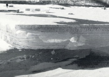
Fig. 1. A block of aufeis formed on a shallow river. Note the ice laminations.
Aufeis formations have long been of interest and concern to scientists and engineers because they cause a variety of engineering problems. For example, they may block drainage facilities, causing subsequent spring flooding and wash-outs of embankments; they may inundate roads, railroads, and airfields causing them to become unusable; they may engulf bridges spanning streams; they may threaten flood-plain communities and individual homes; and they may disrupt operation of tunnels and mines. Further information about aufeis formations occurring in Nature and the problems they cause has been provided byReference Schohl and Ettema Schohl and Ettema (1986a, b), Reference Ashton Ashton (1986),Reference KaneKane (1981), Reference CareyCarey (1973), andReference Alekseyev Alekseyev and others (1973).
2. Experiments
Aufeis was grown in a 0.60 m wide, 0.30 m deep, and 12 m long refrigerated, tilting flume. As aufeis spread and thickened down-stream along the flume, the profiles of the water and ice associated with it were recorded. Figure 2 illustrates schematically a simplified, or idealized, aufeis formation in the refrigerated flume. Because its longitudinal cross-section is invariant across the width of the flume, and its shape is defined by a typical longitudinal, two-dimensional cross-section, the aufeis formation in Figure 2 may be considered two-dimensional. In the experiments, aufeis spread and thickened in a complex, layer-by-layer manner. The early phase of its growth was two-dimensional, but its later growth was influenced by three-dimensional, or boundary, effects.
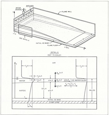
Fig.2. Schematic of two-dimensional aufeis formation in the refrigerated flume. Detail A shows the principal variables associated with aufeis formation.
Figure 2 also illustrates many of the dependent and independent variables associated with aufeis growth. The variables controlled during the experiments include the source-water discharge, Q0; the source-water temperature, ![]() the air temperature, T
a (or heat flux,
the air temperature, T
a (or heat flux, ![]() ); the flume-floor (circulating coolant) temperature,
); the flume-floor (circulating coolant) temperature, ![]() (or heat flux,
(or heat flux, ![]() and the flume slope, S0
. The dependent variables measured during the experiments include the spread length,
and the flume slope, S0
. The dependent variables measured during the experiments include the spread length, ![]() , the thickness of the surface layer of water or slush, d(x,t), and the thickness of aufeis underlying the surface layer,
, the thickness of the surface layer of water or slush, d(x,t), and the thickness of aufeis underlying the surface layer,
For each experiment conducted (36 total), Table I lists the values maintained for the controlled variables, the corresponding values of the key heat-flux components, and the values of four normalization scales (defined in subsequent sections). The heat flux фio
refers to the initial value of the heat flux, ![]() , from the water-ice interface into the underlying aufeis. This heat flux varied with both distance, x, and time, t, during the experiments, because in addition to depending on the flume floor temperature, Tb
, it depends on the thickness of the initial ice base and on' the thickness of aufeis,
, from the water-ice interface into the underlying aufeis. This heat flux varied with both distance, x, and time, t, during the experiments, because in addition to depending on the flume floor temperature, Tb
, it depends on the thickness of the initial ice base and on' the thickness of aufeis, ![]() . One controlled variable not included in Table I is the source-water temperature. For all of the experiments, the temperature of the water supplied to the diffuser was maintained between about 1° and 3°C. Because the water cooled as it flowed through the diffuser, the temperature,
. One controlled variable not included in Table I is the source-water temperature. For all of the experiments, the temperature of the water supplied to the diffuser was maintained between about 1° and 3°C. Because the water cooled as it flowed through the diffuser, the temperature, ![]() , of the water in the pool under the diffuser was maintained between 0° and 0.5 °C. All data obtained from the experiments have been documented by Reference Schohl and EttemaSchohl and Ettema (1986a).
, of the water in the pool under the diffuser was maintained between 0° and 0.5 °C. All data obtained from the experiments have been documented by Reference Schohl and EttemaSchohl and Ettema (1986a).
TABLE I. List Of Experiments
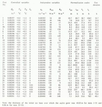
Note: the thickness of the initial ice base over which the aufeis grew was =0.03 m for tests 1–31 and 0.06 m for tests 32–33.
Aufeis growth was initiated by introducing source water to the diffuser. An experiment was terminated either when the aufeis reached the down-stream (free overfall) end of the flume, or when the up-stream depth of aufeis approached the depth of the flume, whichever condition occurred first. As indicated in Table I, the time required for one experiment, from the first release of source water to the end of a test, varied from about 3 to 72 h. At the end of each test, the aufeis was cut to expose and measure the layers of solid and slush ice that characterize cross-sections of aufeis. The experimental apparatus and procedures have been described more fully by Reference Schohl and EttemaSchohl and Ettema (1986a, b).
3. Description Of Aufeis Growth
The growth of a two-dimensional aufeis formation is portrayed sequentially in Figure 3, in which the vertical scale is distorted by approximately one order of magnitude. In Figure 3, Tf
refers to the freezing temperature of water. The normalization scales ts
and ![]() , for which values are listed in Table I, are defined subsequently in section 4.
, for which values are listed in Table I, are defined subsequently in section 4.
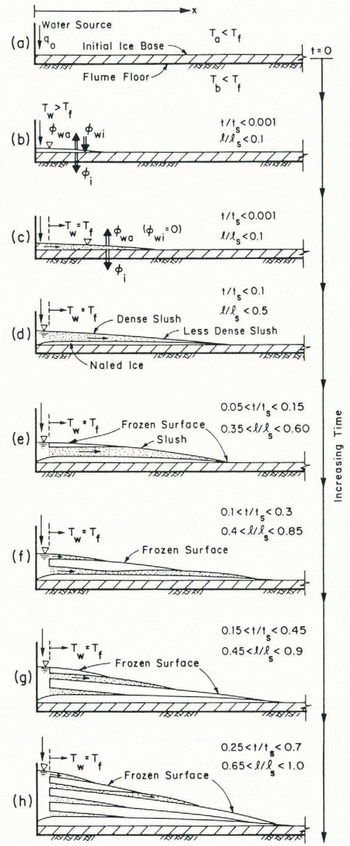
Fig. 3. Sketches illustrating two-dimensional aufeis formation.
Water cooled rapidly to its freezing temperature as it flowed over, and fed, an aufeis formation. Ice crystals, in the form of platelets anchored to the base ice surface, grew into the flow. The accumulation and growth of the ice platelets transformed the free-surface laminar flow of water into a flow through a porous medium composed of ice. Herein, this mixture of ice and flowing water is referred to as aufeis slush. During the experiments, aufeis slush eventually froze at its surface to form a solid crust of ice. Water continued to percolate through the layer of permeable slush, between the thickening ice crust over the slush and the underlying ice surface, until the permeability of the layer was sufficiently reduced to force water to flow over the frozen crust. Another slush layer then began to form. A second crust of ice would eventually form on the new surface flow. The continuing, cyclic process by which ice layers formed on the surface of slush layers resulted in the ice laminations that are a feature of aufeis cross-sections. Depending on the amount of time that the surface layers of ice had for thickening before they were covered by a fresh layer of slush, the laminations sometimes consisted entirely of solid layers of ice and sometimes consisted of alternating solid layers and layers of slush ice.
The flume constrained aufeis so that its initial growth was two-dimensional. However, the surface of the slush always began freezing and solidifying in the central third of its width rather than uniformly across the flume. As the central part hardened and thickened, constricting the flow through the underlying slush, the water was diverted to the sides of the flume so that the slush near the side walls continued to develop. The subsequent aufeis surface was uneven, with a rough, dry center and wet, slushy sides. Strictly speaking, the aufeis was no longer two-dimensional.
4. Normalized Parameters Influencing Aufeis Growth
The dependent variables that describe the growth of laterally confined aufeis, for example, the streamwise spread length (![]() ), the depth of ice-water slush on the surface (d), or the slope of the aufeis surface (S), depend on at least 14 independent variables. If a general dependent variable is designated as
), the depth of ice-water slush on the surface (d), or the slope of the aufeis surface (S), depend on at least 14 independent variables. If a general dependent variable is designated as ![]() , the following functional relationship can be written:
, the following functional relationship can be written:
in which (see Fig. 2) x is streamwise distance, t is time, q0
is unit discharge of water, фша and ![]() are heat fluxes from aufeis surface to air and from surface layer to underlying aufeis, respectively, S0
is slope of base on which aufeis forms, w is lateral width of confined aufeis formation, ρi and ρw are densities of ice and water, respectively, v is kinematic viscosity of water, g is gravitational acceleration, L is latent heat of water fusion, and αi and αw are thermal diffusivities of ice and water, respectively. Because temperature effects are incorporated into the heat-flux components, only three dimensions (length, mass, and time) are contained in the variables in Equation (1). Therefore, the 14 independent variables combine into 11 dimensionless groups, or normalized parameters.
are heat fluxes from aufeis surface to air and from surface layer to underlying aufeis, respectively, S0
is slope of base on which aufeis forms, w is lateral width of confined aufeis formation, ρi and ρw are densities of ice and water, respectively, v is kinematic viscosity of water, g is gravitational acceleration, L is latent heat of water fusion, and αi and αw are thermal diffusivities of ice and water, respectively. Because temperature effects are incorporated into the heat-flux components, only three dimensions (length, mass, and time) are contained in the variables in Equation (1). Therefore, the 14 independent variables combine into 11 dimensionless groups, or normalized parameters.
Reference Schohl and EttemaSchohl and Ettema (1986a) derived, from conservation principles, depth-integrated equations for flow through aufeis slush. Rewritten in appropriate non-dimensional form, these equations indicate the correct form and importance of six of the 11 normalized parameters. The forms of the remaining five parameters are determined from dimensional analysis. In non-dimensional form, Equation (1) becomes
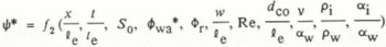
in which ![]() is a normalized dependent variable,
is a normalized dependent variable, ![]()
![]()
![]() where the constant 1010 is included merely for convenience,
where the constant 1010 is included merely for convenience, ![]() , the critical depth in a wide rectangular channel conveying a unit discharge q0
, and
, the critical depth in a wide rectangular channel conveying a unit discharge q0
, and ![]() , a Reynolds number.
, a Reynolds number.
In Equation (2), ![]() , termed the equilibrium length, is a length scale and te
is a commensurate time-scale. The equilibrium length is a theoretical spread length for two-dimensional aufeis, derived by integrating the depth-integrated conservation of mass equation over the length of the aufeis:
, termed the equilibrium length, is a length scale and te
is a commensurate time-scale. The equilibrium length is a theoretical spread length for two-dimensional aufeis, derived by integrating the depth-integrated conservation of mass equation over the length of the aufeis:
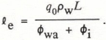
Subject to simplifying assumptions (see Reference Schohl and EttemaSchohl and Ettema, 1986a, b), for this length of spread, the source-water discharge is equal to, or in equilibrium with, the rate at which water is freezing along the aufeis. The time-scale te is defined in terms of the equilibrium length and the source-water discharge, q0 , as follows:
With the value of 100 included, te
represents the time required to cover a unit width of aufeis surface, ![]() in length, with water of average depth
in length, with water of average depth ![]() /100. For all the experiments, average water depths were several orders of magnitude less than values of
/100. For all the experiments, average water depths were several orders of magnitude less than values of ![]() .
.
The length scale ![]() referenced in Figure 3, is defined by Equation (3) with
referenced in Figure 3, is defined by Equation (3) with ![]() omitted. As aufeis accumulates layer by layer, the flow on its surface is often insulated from the heat flux
omitted. As aufeis accumulates layer by layer, the flow on its surface is often insulated from the heat flux ![]() . Consequently, the influence of
. Consequently, the influence of ![]() , though initially significant, diminishes with aufeis thickening. The time-scale ts
is defined by Equation (4) with
, though initially significant, diminishes with aufeis thickening. The time-scale ts
is defined by Equation (4) with ![]() substituted for
substituted for ![]() .
.
Four of the 11 normalized parameters in Equation (2) may be omitted. The three parameters ![]() , and
, and ![]() are omitted because they are essentially constant for ice and water at a temperature near the freezing temperature. The parameter
are omitted because they are essentially constant for ice and water at a temperature near the freezing temperature. The parameter ![]() is omitted because it is associated with the acceleration term in the normalized momentum equation, and this term is negligible for seeping flow through aufeis slush. The functional relationship containing the key variables influencing aufeis growth is
is omitted because it is associated with the acceleration term in the normalized momentum equation, and this term is negligible for seeping flow through aufeis slush. The functional relationship containing the key variables influencing aufeis growth is
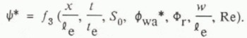
The laboratory data on the spreading and thickening of aufeis are presented below in terms of the parameters in Equation (5). Because, as mentioned above, ![]() varied with x and t, the initial values of
varied with x and t, the initial values of ![]() and
and ![]() , designated as
, designated as ![]() and t
e0, are used to normalize length and time variables.
and t
e0, are used to normalize length and time variables.
5. Aufeis Spreading
In its initial phase of growth (Fig. 3b), aufeis spread relatively quickly. The growth and accumulation of ice platelets, which removed water mass and impeded the flow, gradually slowed aufeis spreading (Fig. 3c and d). As its surface froze into a layer of solid ice and a second layer of slush formed (Fig. 3e and f), aufeis spread intermittently, stopping for periods of time and then continuing. Aufeis sometimes stopped spreading for relatively long periods of time when either its length approached its time-varying equilibrium length, or as the slush froze solid near its down-stream end (Fig. 3g and h). Often, a fresh slush layer would later spread over and beyond the down-stream frozen surface, thereby continuing the aufeis expansion.
Aufeis spreading is described by Equation (5) with ![]() replaced by normalized spread length,
replaced by normalized spread length, ![]() . Because it is not a function of
. Because it is not a function of ![]() , spread length is influenced by six of the seven independent parameters in Equation (5). In Figure 4a–c, the experimental data for aufeis spreading on initially horizontal slopes (S0
= 0) are plotted against log of normalized time. In each plot, the values of base slope, S0
, and normalized heat flux,
, spread length is influenced by six of the seven independent parameters in Equation (5). In Figure 4a–c, the experimental data for aufeis spreading on initially horizontal slopes (S0
= 0) are plotted against log of normalized time. In each plot, the values of base slope, S0
, and normalized heat flux, ![]() , are the same for all tests represented. Therefore, in accordance with Equation (5), the data in each plot should separate consistently with variations in
, are the same for all tests represented. Therefore, in accordance with Equation (5), the data in each plot should separate consistently with variations in ![]() , and Re for those cases in which these variables influence spreading. Curves representing the data plotted in Figure 4a–c are plotted together in Figure 5 in order to illustrate the influence on aufeis spreading of the normalized surface heat flux,
, and Re for those cases in which these variables influence spreading. Curves representing the data plotted in Figure 4a–c are plotted together in Figure 5 in order to illustrate the influence on aufeis spreading of the normalized surface heat flux,
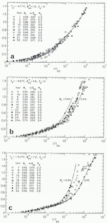
Fig. 4. Experimental data on aufeis spreading over a horizontal slope: (a) Ta = −4.7°C; (b) Ta = −9.8°C; (c) Ta = −13.2° C
During the early phase of aufeis growth (Fig. 3b–d), before the surface of the slush layer freezes solid, the normalized rate at which aufeis spreads is influenced by variations in
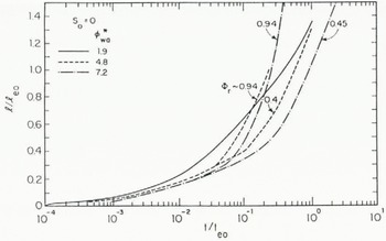
Fig. 5. Influences of
Figure 4b and c show that the data eventually diverge from the common curves corresponding to the early phase of aufeis growth. Figures 4 and 5 together indicate that the point of divergence is influenced primarily by the heat flux ![]() ; that is, aufeis freezes over (or reaches the phase shown in Figure 3e) more rapidly when formed under conditions of larger
; that is, aufeis freezes over (or reaches the phase shown in Figure 3e) more rapidly when formed under conditions of larger ![]() . Figure 4b and c show that, although other influences may be present, the point of divergence for each curve varies with
. Figure 4b and c show that, although other influences may be present, the point of divergence for each curve varies with ![]() : the larger the value of
: the larger the value of ![]() , or the larger value of
, or the larger value of ![]() relative to the total heat loss
relative to the total heat loss ![]() , the sooner, in terms of t/t
e0, the data diverge from the initially common curve. Figure 5 shows that, for equal
, the sooner, in terms of t/t
e0, the data diverge from the initially common curve. Figure 5 shows that, for equal ![]() , the data diverge more rapidly with larger values of
, the data diverge more rapidly with larger values of

Apparently, near the transition value of t/t
s, the magnitude of the heat flux ![]() is effectively reduced over part of an aufeis formation’s surface. Consequently, less of the water supplied to the aufeis freezes and the rate at which aufeis spreads is increased relative to the common curve representing the early phase of growth. The exact reason for the effective reduction in
is effectively reduced over part of an aufeis formation’s surface. Consequently, less of the water supplied to the aufeis freezes and the rate at which aufeis spreads is increased relative to the common curve representing the early phase of growth. The exact reason for the effective reduction in ![]() when t/t
s passes 0.035 is not clear from the data. However, because the transition time is in terms of t
s, the reduction must be related to the increasing accumulation of ice platelets. It seems that, as time increases beyond the transition value of t/t
s, an increasingly significant part of the heat flux from the surface of aufeis acts to reduce the temperature within exisiting ice platelets rather than acting to cause more ice to grow within the slush. This effect leads to a decrease in the rate at which ice platelets grow. The transition value of t/t
s possibly represents the beginning of a continuous transition from the early, maximum rate of growth of ice platelets to the eventual slower rate of growth that occurs after the slush surface freezes over and partially insulates the underlying wet slush from the cold air above. If this is the case, the transition value of t/t
s may correspond to the start of the process by which the slush freezes solid.
when t/t
s passes 0.035 is not clear from the data. However, because the transition time is in terms of t
s, the reduction must be related to the increasing accumulation of ice platelets. It seems that, as time increases beyond the transition value of t/t
s, an increasingly significant part of the heat flux from the surface of aufeis acts to reduce the temperature within exisiting ice platelets rather than acting to cause more ice to grow within the slush. This effect leads to a decrease in the rate at which ice platelets grow. The transition value of t/t
s possibly represents the beginning of a continuous transition from the early, maximum rate of growth of ice platelets to the eventual slower rate of growth that occurs after the slush surface freezes over and partially insulates the underlying wet slush from the cold air above. If this is the case, the transition value of t/t
s may correspond to the start of the process by which the slush freezes solid.
At and beyond their divergence points, the curves in Figure 4b and c do not, in all cases, consistently separate in accordance with variations in Фг. This is attributed primarily to the influence on aufeis spreading of lateral boundaries (flume side walls) after the slush on the aufeis surface begins to freeze solid. As already mentioned, the aufeis slush usually froze first along the central one-third of the flume’s width. When this occurred, some of the up-stream water flow spread over the frozen area, while the remainder was diverted toward the flume’s side walls, away from the frozen area. The water in the slush near the flume’s side walls could flow past the frozen slush in the center of the flume and contribute to the spreading of the aufeis down- stream. The parameter ![]() accounts, at least partially, for the influence of lateral boundaries. Figure 4b and c reveal that, if two sets of data with nearly the same value of Фг are compared (such as tests 5 and 23 in Figure 4b or 17 and 26 in Figure 4c), the data associated with lesser values of
accounts, at least partially, for the influence of lateral boundaries. Figure 4b and c reveal that, if two sets of data with nearly the same value of Фг are compared (such as tests 5 and 23 in Figure 4b or 17 and 26 in Figure 4c), the data associated with lesser values of ![]() lie above the data for which
lie above the data for which ![]() is larger. These results indicate that narrower aufeis formations spread faster, in normalized terms, than do wider aufeis formations.
is larger. These results indicate that narrower aufeis formations spread faster, in normalized terms, than do wider aufeis formations.
For the relatively narrow range of Reynold’s numbers, Re, attained during the experiments, no consistent effect due to variations in Re are discernible in the data. The effect of Re would cause variations in the resistance to flow through aufeis slush, which is most significant during the early phase of growth. However, the data indicate that the early phase of aufeis growth is not affected by variations in Re.
Data collected for two initial slopes of the laboratory flume are compared in Figure 7a and b. Figure 7a compares data from aufeis formed when S 0 = 0.01 and average
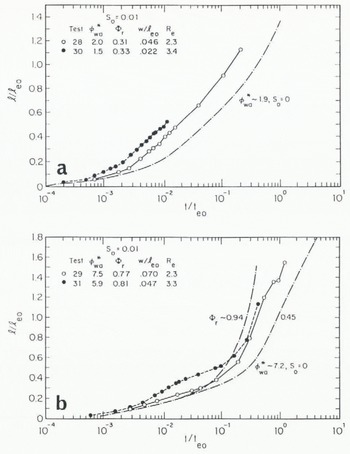
Fig. 7. Comparison of dala on aufeis spreading over two slopes, S0 = 0 and 0.01: (a)![]() ; (b)
; (b) ![]() .
.
6. Aufeis Profile
Aufeis thickening is described by Equation (5) with ψ* replaced by normalized thickness, ![]() . The longitudinal profile of a two-dimensional formation of aufeis is described in terms of overall thickness, s, as a function of streamwise distance, x (Fig. 2). Thickness 5 includes only the water and ice that accumulated during a test; it does not include the thickness of the underlying ice base preformed over the flume floor.
. The longitudinal profile of a two-dimensional formation of aufeis is described in terms of overall thickness, s, as a function of streamwise distance, x (Fig. 2). Thickness 5 includes only the water and ice that accumulated during a test; it does not include the thickness of the underlying ice base preformed over the flume floor.
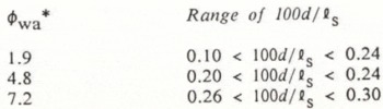
As is the case for aufeis spreading, for times less than the transition value of t/t
s (about 0.035), aufeis is influenced by фwа* but is not affected by variations in Фг, ![]() , or Re. This is evident in Figure 8a–c, which illustrate that the longitudinal shapes of aufeis formed in the flume for normalized times less than the transition time depend only on t/t
e0 and Фwа*. Comparison of Figure 8a–c reveals that, for a given value of t/t
e0, aufeis thickness relative to aufeis length increases with increasing Ф
wа*. In each plot in Figure 8, the values of base slope, S0
, and normalized heat flux, Ф
wа*, are the same for all data included. Therefore, the data in each plot represent aufeis spreading at identical normalized rates (see Figs 4 and 5). The indicated values of t/te0
are averages of the normalized times associated with the data on each curve. The point at which each curve intersects the abscissa corresponds to the appropriate spread length taken from Figure 4.
, or Re. This is evident in Figure 8a–c, which illustrate that the longitudinal shapes of aufeis formed in the flume for normalized times less than the transition time depend only on t/t
e0 and Фwа*. Comparison of Figure 8a–c reveals that, for a given value of t/t
e0, aufeis thickness relative to aufeis length increases with increasing Ф
wа*. In each plot in Figure 8, the values of base slope, S0
, and normalized heat flux, Ф
wа*, are the same for all data included. Therefore, the data in each plot represent aufeis spreading at identical normalized rates (see Figs 4 and 5). The indicated values of t/te0
are averages of the normalized times associated with the data on each curve. The point at which each curve intersects the abscissa corresponds to the appropriate spread length taken from Figure 4.
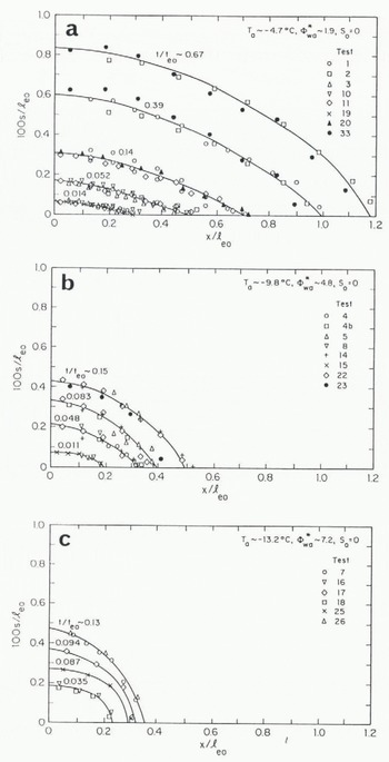
Fig. 8. Profiles of aufeis, presented in terms of normalized parameters for times not exceeding transition lime: (a) Ta = −4.7°C; (b) Ta = −9.8°C; (c) Ta = −13.2°C.
Figures 9a and b, and 10a and b illustrate that, for times larger than the time associated with the transition value of t/t
s, the shape of an aufeis formation is influenced by ΦΓ in addition to t/te0
, Φ
wa*, and S
0. For each plot in these figures the parameters S0
, Ф
wa*, and Фr are the same for all data included. Consequently, if the possible influence of ![]() and Re are neglected, the data in each plot represent aufeis formations spreading at identical normalized rates. For average
and Re are neglected, the data in each plot represent aufeis formations spreading at identical normalized rates. For average
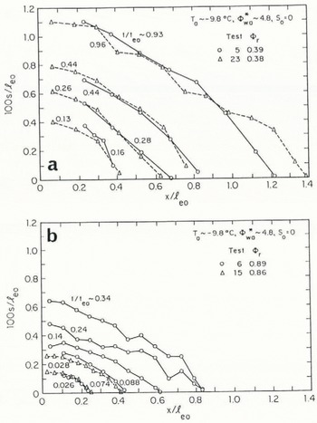
Fig. 9. Aufeis profiles presented in terms of normalized parameters, for times exceeding transition time: T a = −9.8°C; (а Φr = 0.38; (b) Φr = 0.87.
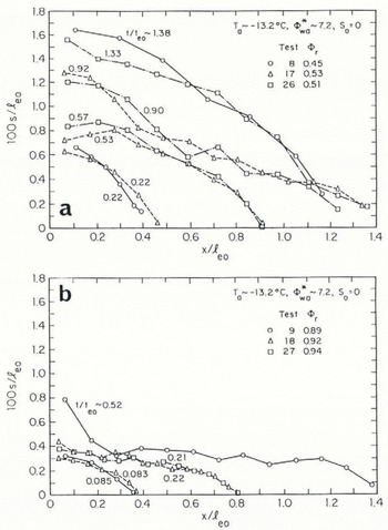
Fig. 10. Aufeis profiles presented in terms of normalized parameters. for limes exceeding transition time: T a = −13.2°C; (а) Фr = 0.45–0.53; (b) Фr = 0.89–0.94.
The possible influence on the data of the parameters ![]() and Re is not evident in Figures 8–10. However, the parameter
and Re is not evident in Figures 8–10. However, the parameter ![]() must influence the longitudinal shape of aufeis because, as discussed in section 5, it influences the length of aufeis spreading.
must influence the longitudinal shape of aufeis because, as discussed in section 5, it influences the length of aufeis spreading.
As illustrated by the data associated with the largest values of t/t e0 in Figures 9 and 10, the surface of aufeis often became uneven after the slush on its surface began to freeze solid. A feature of aufeis formation that is not evident in the profiles presented in Figures 8–10 is ledging, or the stepped profile which characterizes the front of many aufeis formations. In the refrigerated flume, under conditions of constant air temperature and water flow, ledging was observed only at the down-stream front of spreading aufeis, as illustrated in Figure 11 (an aufeis formation formed under conditions similar to those in tests 8 and 32).
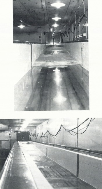
Fig. 11. Views of aufeis formed in the flume. Mild ledging is evident at the front of the aufeis.
7. Aufeis Lamination Thickness
As described in section 3, aufeis grows as successive layers of slush form and freeze solid into laminations of ice. Comparisons of measured values of lamination thickness with measured values of slush depth indicate that the thickness of an ice lamination is equal to the maximum depth attained by the slush from which the lamination developed. Therefore, data on slush depth indicate thicknesses of ice laminations in aufeis.
Besides being influenced by each of the key parameters given in Equation (5), the depth of a layer of aufeis slush may be affected by its position in the sequence of formation of slush layers. The data presented in this section were taken from the first layer of slush that developed after aufeis growth was initiated in the refrigerated flume.
The depth of the initial layer of slush, d, equals the thickness of the aufeis, s, minus the thickness of accumulated bottom ice, η (Fig. 2). The normalized depth of slush, d/le0
varies with ![]() ,
, ![]() and
and
Table II indicates the maximum depths attained by slush layers near the up-stream end of the flume. These depths should equal the thickness of subsequent ice laminations. The time at which the slush up-stream reached a maximum depth ranged from t/t s = 0.06 to 0.10. At some time within this range, the surface of the slush up-stream froze sufficiently to stop the thickening of the initial layer of slush. The maximum depth of slush decreased with increasing distance over aufeis but enough data to describe this variation are available only for
TABLE II. Maximum Depth Of Slush Up-Stream![]()
Maximum slush depth, d, and corresponding time, t, are normalized by ![]() and t
s rather than
and t
s rather than ![]() and t
e0 in order to minimize the influence of Фr. In fact, the quantity of data is not sufficient to identify any consistent variations with Φr in either the maximum value of
and t
e0 in order to minimize the influence of Фr. In fact, the quantity of data is not sufficient to identify any consistent variations with Φr in either the maximum value of ![]() or in the corresponding value of t/t
s.
or in the corresponding value of t/t
s.
The slush layers developing after the initial layer were nearly as deep as the initial layer. This observation suggests that little water flowed through slush layers under the surface of an aufeis formation. The succeeding layers formed from nearly as much water flow as did the initial layer.
8. Scales
In section 4, ![]() and t
e0, the initial values of
and t
e0, the initial values of ![]() and t
e, are introduced as length and time scales for normalizing and, therefore, describing aufeis formation. Only the initial values of
and t
e, are introduced as length and time scales for normalizing and, therefore, describing aufeis formation. Only the initial values of ![]() and t
e are convenient to use because the heat flux to the frigid base,
and t
e are convenient to use because the heat flux to the frigid base, ![]() , diminishes over time, gradually increasing the values of le and t
e until, in the limit, these scales are equivalent to ls and t
s, which are length and time scales derived by neglecting
, diminishes over time, gradually increasing the values of le and t
e until, in the limit, these scales are equivalent to ls and t
s, which are length and time scales derived by neglecting ![]() . The usefulness of le0and te0 in describing aufeis geometry, particularly during the early phase of aufeis growth, is verified in the figures presenting the laboratory data on spreading and thickening of two-dimensional aufeis (e.g. Fig. 4). Use of ls and ts, as is done in Figure 3, may be appropriate for describing the layer-by-layer phase of aufeis growth, after the transition time has passed, or, more generally, when
. The usefulness of le0and te0 in describing aufeis geometry, particularly during the early phase of aufeis growth, is verified in the figures presenting the laboratory data on spreading and thickening of two-dimensional aufeis (e.g. Fig. 4). Use of ls and ts, as is done in Figure 3, may be appropriate for describing the layer-by-layer phase of aufeis growth, after the transition time has passed, or, more generally, when ![]() is much greater than
is much greater than ![]() . By themselves, however, neither le0 and te0 nor ls and ts are sufficient to describe aufeis formation.
. By themselves, however, neither le0 and te0 nor ls and ts are sufficient to describe aufeis formation.
The scales le0 and te0 are derived from integration of the conservation-of-mass equation for flow over the surface of aufeis. Consequently, these scales normalize differences in total mass between aufeis formations, where normalized total mass per unit width of aufeis, M*, is defined as follows:
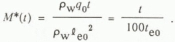
As is evident from Equation (6), at any given value of normalized time, t/t
e0, all two-dimensional aufeis formations consist of the same quantity of normalized mass. Further more, for all aufeis formations spreading at the same normalized rate (l/le0 as a function of t/te0
), the division of the total normalized mass into ice mass, Mi*, and water mass, Mw*, is the same. This is evident from the following equation for normalized ice mass, Mi*, derived by Reference Schohl and EttemaSchohl and Ettema (1986a) for constant total heat flux, ![]() :
:
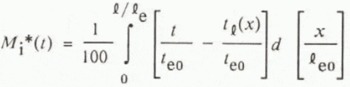
in which Mi is ice mass per unit width and tl(x) is time at which the spreading, down-stream edge of aufeis reaches streamwise position x. Because the mass of unfrozen water is the difference between the total mass and the total ice mass, aufeis formations consisting of the same M* and Mi* also contain the same Mw*.
While the total quantity of ice is accounted for using the scales le0 and te0, they do not take into account the division of ice into ice platelets, which grow to balance the heat flux ![]() , and bottom ice, which grows to balance the heat flux
, and bottom ice, which grows to balance the heat flux ![]() . Effects that depend on one or the other of these heat fluxes, rather than the total heat flux, vary with Фг and
. Effects that depend on one or the other of these heat fluxes, rather than the total heat flux, vary with Фг and
Figure 8 shows that aufeis formations spreading at the same normalized rate have the same longitudinal shape at any given time, t/t e0, before the transition time has passed. That is, not only do they have the same normalized mass, as mentioned above, but the distribution of the mass over x/le0 is also the same. However, Figure 8 also shows that, before the transition time has passed, aufeis thickness relative to aufeis length increases with increasing
The foregoing discussion deals with definition of appropriate scales for describing two-dimensional formations of aufeis. For description of three-dimensional formations, such as may form at the exit of a culvert or over a broad, shallo w river, different length and time scales would apply. Appropriate scales would entail use of a theoretical spread area from which would be determined length as well as time-scales.
9. Conclusions
The many factors influencing aufeis growth reduce to a set of seven key independent parameters as expressed in Equation (5).
A transition time is identified which apparently coincides with the beginning of the processes by which the initial layer of ice-water slush on aufeis freezes solid. In terms of the time-scale t s this transition time is approximately t/t s = 0.035. However, the transition time may vary slightly with
The early phase of aufeis formation, before the transition time has passed, is influenced by only the first four key parameters listed in Equation (5). For the same values of S 0 and
After the transition time has passed, Фr and w/l e of the remaining three parameters in Equation (5) come into play. The normalized rate of aufeis spreading increases with increasing Фr and with decreasing w/l e (Fig. 4). At a given value of t/t e, aufeis forming under large Фr is both longer and thinner than aufeis formed under smaller Фr (Figs 4, 9, and 10). The data from aufeis formed on a sloped surface suggest that, after the transition time has passed, the rate at which aufeis spreads may no longer depend on slope, S 0 (Fig. 7).
Although it is possible that variations in Reynolds number, Re, also influence aufeis formation, for the relatively narrow range of Reynolds numbers attained during the experiments, no consistent effect is discerned.
The thickness of aufeis laminations corresponds to the thickness attained by slush layers before they freeze solid.
The present study is limited to two-dimensional aufeis formations such as those, for example, that may develop inculverts. Considerable work remains before relationships are available for use in the design of culverts and other watercourses for the possibility of aufeis formation. Further work is also needed on aufeis formations which spread and thicken three-dimensionally.
Acknowledgement
This research was supported by the U.S. National Science Foundation (NSF grant CEE81–09252).


