Constitutive equations

We shall write Glen’s law in the form

where σ′ _ij = σ _ij + pδ _ij is the deviatoric stress tensor formed by subtracting the mean normal (hydrostatic) pressure pδ _ij from the actual stress tensor σ _ij , and e _ij is the strain-rate tensor. The generalized viscosity μ is a function of θ, the second strain-rate invariant defined by

θ is related to τ, the second invariant of the deviatoric stress, defined by

by the power-law relation

where the power n is a constant ≃ 3, whilst B is a function of temperature. It follows from Equations (1) to (4) that the viscosity function is given by

When n > 1, the power law represents a strain-rate softening material and so μ is a decreasing function of θ Estimated values of B, averaged through the ice thickness, have recently been given by Reference Thomas and MacAyealThomas and MacAyeal (1982) for the Ross Ice Shelf.

The zeroth-order solution

Reference WeertmanWeertman’s (1957) analysis assumes an ice shelf of constant thickness h, with parallel top and bottom surfaces, deforming under plane-strain conditions. The bottom surface is at a depth ρ _i h/ρ _w below mean sea-level where ρ _i and ρ _w are the (mean) densities of ice and sea-water, respectively. Weertman demonstrated the existence of a simple steady-state solution in which the strain-rate components are uniform. This is going to be our zeroth-order solution about which we will consider small perturbations. With the notation of Figure 2, the zeroth-order strain-rates

The constant creep-rate K is positive if the ice shelf is extending and negative if it is compressing in the flow direction. The zeroth-order strain-rate invariant θ⁽⁰⁾ = │K│. The plane-strain assumption requires σ _yy ⁽⁰⁾ = (σ _xx ⁽⁰⁾ + σ _zz ⁽⁰⁾)/2 from Equation 1, so that the zeroth-order stress invariant

.

Fig. 2. Notation.

Thus from Equations (4) and (5)

Since the x-, y-, and z-directions are principal strees directions,

and the equilibrium equations reduce to

Solving Equations (7) and (8), and using the stress-boundary conditions on the upper (σ_zz ⁽⁰⁾(h) = 0) and lower (σ_zz ⁽⁰⁾(0) = − ρ _i gh) surfaces, gives

This solution will be assumed to describe the local background stress and strain-rate states in the ice shelf. The resultant compressive force acting through the shelf is

Weertman equated this to the total force of the sea-water on the ice front, i.e. to ρ _i ² gh ²/2ρ _ω, and so obtained an expression for the creep-rate K. However, here we will follow Reference ThomasThomas (1979) and allow for the addition of a “back pressure” P which arises from the resistance of ice rises and the shelf margins. So from Equation (10) the creep-rate K is given by

where Δρ = (1 − ρ _i/ρ _ω). When P = 0, K is positive and the shelf is extending; compressive flows will occur however when the back pressure exceeds ½ρ _iΔρgh. Reference Thomas and MacAyealThomas and MacAyeal (1982) have plotted contours of the resisting force F = Ph on the Ross Ice Shelf obtained from the RIGGS data.

Perturbation equations

The stress and strain-rate fields in the buckled ice shelf will be regarded as the sum of the above zeroth-order solution together with perturbed fields denoted by

and e_ij . The viscosity function is hence

where µ₀′ stands for dµ/dθ evaluated at θ = θ⁽⁰⁾, which from Equation (5) is given by

The first-order perturbed strees and strain-rate fields are related by

using Equations (1) and (12). The perturbation in the second strain-rate invariant is

using the standard Taylor series expansion; but

obtained by differentiating Equation (2), so that

In the zeroth-order solution all the strain-rate components are zero except for

and in the perturbed solution ẽ_xx = −ẽ_zz , since the deformation is still assumed plane strain, so that Equation (15) can be rewritten

Finally, substituting from Equation (13) and (15ʹ) into Equation (14) gives the perturbed stresses as

where

is the value of the hydrostatic stress in the perturbed stress field.

The “shear viscosity” relative to the x, z-axes is hence µ ₀ the value in the background state, but the “extensional viscosity” is reduced to µ ₀/n due to the pure compression/extension in the x, z-directions in the ground state. The ice will hence offer less resistance to further extension or compression in the horizontal and vertical directions than it will to shearing in the vertical plane. This kind of “stress-induced anisotropy” is of course a characteristic feature of non-linear materials.

Since the perturbed deformation is isochoric, we can introduce a stream function ψ (x, z) such that the velocity components are (ũ,

) where

The strain-rate components are found by differentiation and when substituted in Equation (16) gives the stress components

Substituting these expressions in the perturbed equilibrium equations

yields the following expressions for the pressure gradients

Finally, eliminating p gives the fourth-order equation

for the stream function ψ. This is the anisotropic biharmonic equation which governs the plane-response behaviour of anisotropic elastic solids (see Reference BiotBiot, 1965). It reduces to the ordinary biharmonic equation ∇²(∇² ψ) = 0 for a Newtonian viscous model with n = 1.

Boundary conditions

The perturbed shape and motion of the shelf will be obtained by solving Equation (21), subject to suitable boundary conditions on the upper and lower surfaces, which we shall denote by z = h + ξ(x, t) and z = η(x, t) respectively (Fig. 2), where

.

The normal and shear-traction components on the upper surface are zero, so choosing local normal and tangential coordinates (Fig. 2)

The x, z stress components can be obtained by the usual rules for the rotation of stress components and can be written in terms of the only non-zero local direct stress σ _tt :

where θ = ξ, _x is the surface slope. Working to first order in θ, we see that

Applying the first of these conditions

on the deforming surface z = h + ξ and using the Equations (9) for σ _zz ⁽⁰⁾, we obtain the boundary condition

Similarly, the second condition in Equations (23′) gives the boundary condition in the shear stress

These conditions can be put in terms of the stream function ψ by using Equation (18)

and

Differentiating Equation (24′) with respect to x, eliminating p,_x from the equilibrium Equation (20), and finally eliminating ξ, _x from Equation (25′) gives one boundary condition on ψ on the upper surface, z = h:

where σ is the dimensionless stress coefficient defined by

An analogous argument can be used to find a boundary condition on the lower surface. The presence of the sea-water pressure means that Equation (24) is replaced by

. The rest of the derivation goes through similarly and Equation (26) is replaced by

where

The remaining two boundary conditions come from the usual kinematic condition in linear wave problems, namely, that the rate of change of surface elevation is equal to the vertical velocity component on each surface, i.e.

Following Reference BiotBiot (1965) and Reference SmithSmith (1977), we now look for disturbances which are growing exponentially with a growth-rate G. So that

where f and g are amplitude functions, and

so that the kinematic conditions in Equation (30) become

Finally, differentiating these expressions with respect to x and eliminating ξ or η from Equations (25′), we obtain the remaining two boundary conditions on ψ

We thus have a determinate problem for the perturbed motion: to solve the anisotropic biharmonic Equation (21) for ψ subject to boundary conditions in Equations (26), (28), and (33).

Wave solutions

We now seek solutions to this system of equations in the form of a uniform train of waves with wave number k, so that ξ, η, ψ, and all the other perturbation variables vary with x as exp(ikx). In particular,

We assume k is real so that the wave train is not damped. In effect we are solving the problem for an infinitely long shelf. Substituting Equation (34) into the governing Equation (21) gives a linear fourth-order ordinary differential equation for Φ(z) with solutions of the form exp(νkz) where ν satisfies the quartic equation

where ω = (2 − n)n, so that ν takes one of the four values ν _j , j = 1,2,3,4;

For n < 1, these roots are all real and distinct, for n = 1 there are two repeated roots (± 1) and for n > 1 there are two sets of complex conjugate roots. In the limit as n → ∞, corresponding to a perfectly plastic material, Equation (36) has two repeated pure imaginary roots (± 1). For ice with n ≃ 3 the variation of ψ through the shelf thickness is hence the sum of four damped oscillations.

Determination of wavelengths

Substituting Equation (37) into the four boundary conditions in Equations (26), (28), nd (33) yields a set of four linear homogeneous equations for the vector a of coefficients a_j of the form

where the elements of the rows of the (4 × 4) matrix B are

for j = 1,2,3,4.

The ice shelf can buckle and waves form if Equation (38) has a non-zero solution for a, i.e. if B is singular and

This can be regarded as an equation determining the non-dimensional growth rate

as a function of

• (i) dimensionless wavelength λ = 2π/kh,

• (ii) stress coefficient σ = 2μ₀ K/ρ_i gh,

• (iii) density ratio Δρ = (1 − ρ _i/ρ _w)

• (iv) the creep-law index n,

i.e.

Equation (40) is quadratic in (G/K), so that the equation could be constructed by evaluating det B (which is always real) for three different growth-rates and then solved analytically. It was found that the roots for γ were always real and either both negative or with one root negative and the other positive. A negative growth-rate implies that the disturbance dies away and the ice shelf is stable. We are herfe principally concerned with the positive growth-rate solution.

Critical stress regimes

The variation of growth-rate with stress coefficient for various wavelengths is illustrated in Figure 3. Three separate regimes can be distinguished.

Fig. 3. Variation of non-dimensional growth rate γ with stress coefficient Σ for various values of non-dimensional wavelength n, (n = 3 and ρ_i/ρ_w = 0.75). The critical formation wavelength for a given value of σ is that with the largest growth-rate and hence is given by the envelope to the above curves.

• (i) For sufficiently small stress coefficients in the range − σ _c < σ < σ _e the growth-rate is always negative irrespective of the wavelength. Thus in this regime the ice shelf is stable and all disturbances will be damped out.

• (ii) In an extending flow region with σ > σ _e , positive growth-rates occur, but these are a monotonically increasing function of wavelength. Thus the wavelength with the largest growth-rate is theoretically infinite. This means that the ice shelf will tend to respond to perturbations by thinning or thickening uniformly over its entire length. Thus again in this regime one would not expect waves to grow.

• (iii) For a sufficiently large compressive stress coefficient, so σ < − σ _c , the growth-rates are positive and have a maximum at a definite critical wavelength which depends on the value of σ. Thus in this regime one would expect waves of a definite finite wavelength to form. It is to be noted that even in this regime waves with a non-dimensional wavelength less than about 2 have negative growth-rates, so that this theory predicts that only waves whose initial wavelength is greater than about twice the local ice thickness can form under any circumstances. As shown in Figure 4, the critical formation wavelength Figure 4, 5 and 6 increases from around 2 when σ = −σ _c = − 0.3 to 6 when σ = − 2.0 and 8 when σ = − 4.0. As shown in Figures 5 and 6, the critical wavelength has only a slight dependence on n but the value of the critical stress coefficient σ _c decreases significantly as n or the density ratio ρ _i/ρ _w is increased.

Fig. 4. Variation of non-dimensional growth rate Y with stress coefficient σ (for negative σ) for various values of non-dimensional wavelength λ (n = 3 and ρ_i/ρ_w = 0.75).

Fig. 5. a. Variation of critical formation wavelength with stress coefficient for various values of creep index n.

b. Variation of formation growth-rate with stress coefficient for various values of creep index n(ρ_i/ρ_w = 0.75).

Fig. 6. Variation of critical stress coefficient −σ_c, at which waves can first form, with density ratio ρ_i/ρ_w for various values of creep index n.

Critical back pressures

The stress coefficient σ is a measure of the deviatoric stress in the shelf. It is related to the “back pressure” P by the formula

which is obtained by eliminating the strain-rate K between Equations (11) and (27). Thus for waves to form the back pressure must exceed the cirtical value P_c , where

Estimates of the values of the stress coefficient σ in the Ross Ice Shelf can be made from the data on back pressure given by Reference Thomas and MacAyealThomas and MacAyeal (1982) and ice thickness by Reference Bentley, Bentley, Clough, Jezek and ShabtaieBentley and others (1979). Values vary from 0.08 at the ice front, where the back pressure P = 0 to around 0.00 at Crary Ice Rise or behind Roosevelt Island, where the retarding force F = Ph ~ 2 × 10⁸ N m⁻¹ and the ice thickness is 500–550 m. These estimates of σ are hence never compressive; they are however obtained by averaging data over a relatively large area. Here we require more localized information obtained from the neighbourhood of pressure ridges. For the two folds near Camp Michigan, Reference KehleKehle (1964) estimated the value of the stress coefficient to be −1.9, which is well into the region where waves can be expected to form (Figs 3 or 4). Similarly, preliminary estimates (see later) in the region where the Pram Point pressure ridges are forming on the McMurdo Ice Shelf give compressive stress coefficients of the order of −1.3.

The above analysis is two-dimensional assuming the ice shelf is deforming under plane-strain conditions. However, as will be shown in the next section, the presence of lateral strain-rates can have a significant effect on the stability of the shelf. Further discussion of the comparison of the theory with available field data is hence delayed until after this extension of the theory has been presented.

A note on the impossibility of wave propagation

In the above analysis it has been shown that, if one looks for solutions which vary as exp(Gt) with time and exp(ikx), then the growth-rate G and wave number k are simultaneously real. Similarly, solutions which are periodic in time, varying as exp(iωt), have real exponential variations with distance. It is hence impossible to find propagating wave solutions, varying as exp i(ωt − kx). This is not surprising in view of the quasi-static nature of the theory. As noted by Reference ThompsonThompson (1979), it would be necessary to include the inertia terms in the equation of motion in order to study the possible development of progressive waves. This has not been attempted here.

Zeroth-order solution

Reference ThomasThomas (1973) generalized Weertman’s steady-state solution to allow for lateral straining the in the y-direction. The zeroth-order strain-rates in Equation (6) are now replaced by

where

is the ratio of lateral to longitudinal strain-rates. The previous theory can be modified to study the effect of lateral strain-rates on the growth of wave instabilities. The axes of the waves are still assumed to be normal to the x-principal strain-rate direction. The second strain-rate invariant is now

and the zeroth-order viscosity is

From the flow rule in Equation (1) the principal stress difference

Since σ _zz ⁽⁰⁾ is still given by Equation (9) by equilibrium,

Integrating through the ice thickness and introducing the back pressure P and stress coefficient σ as before, we obtain the modified form of Equation (42):

The effect of lateral spreading is hence to introduce the (1 + ½α) term on the left-hand side. It is important to note that if α < − 2, σ will have the opposite sign to the right-hand side of Equation (51). For example, at the seaward edge of an ice shelf, where P = 0, it is possible to have a compressive strain-rate (K < 0) in the x-direction (normal to the ice front) provided the magnitude of the lateral extensional strain-rate in the y-direction is greater than 2│K│.

Perturbation analysis

The perturbation analysis proceeds in exactly the same way as before. Since the magnitudes of the zeroth-order strain-rates in the x- and z-directions are no longer equal, the “effective viscosities” for superposed deformations in these directions are now different. The perturbed stress/strain-rate Equation (16) are replaced by

where

Both expressions reduce to μ₀/n when α = 0 and to μ₀ when n = 1.

Introducing a stream function and substituting in the equilibrium equations, we again arrive at the anisotropic biharmonic Equation (21) but with n replaced by n′, where

The anisotropies introduced by the non-linear power law and the different background strain-rates are hence combined in the single parameter n′. The derivation of the boundary conditions proceeds as before and again it is found that the only modification to Equations (26) and (28) is that n replaced by n′.

The variation of n′ with σ for various values of n, as given by Equation (54), is shown in Figure 7. As α increases from zero, the value of n′ decreases monotonically to 4n/(3 + n) when α = 1 and tends asymptotically to 4n/(1 + 3n) as α → ∞. The value of n′ also decreases initially for negative values of α, reducing to 4n/(1 + 3n) when α = −1 and to 1 (for all n) when α = −2; it then increases again slightly to 4n/(1 + 3n) as α → − ∞. In no case is the value of n′ less than unity.

Destabilizing effect of lateral straining

The variation of the critical stress coefficient at which buckling occurs σ _c with α can be determined by combining Figures 6 and 7. In general, the value of σ_c increases with |α|. However, the effect of lateral straining on the onset of buckling is best illustrated in Figure 8 where the value of the non-dimensional critical back pressure P_c /ρ _i gh, given by Equation (51), is plotted against −α for n = 3 and for various density ratios. For α in the range 0 to −1 there is only a small decrease in the critical back pressure. This is because the reduction in P_c caused by the (1 + ½α) term in Equation (51) is more or less balanced by the increase in the value of σ_c caused by the increase in|α|. However, the first effect is dominant when α < −1 and P_c /ρ _i gh decreases to ½Δρ when α = −2 and then becomes zero at some value between −2.3 and −2.5 depending on the density ratio.

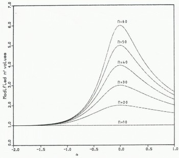
Fig. 7. Variation of “effective” creep index n′ with lateral straining coefficient

for various values of creep index n.

Fig. 8. Variation of critical back pressure P_c, at which waves can be expected to form, with the lateral straining coefficient α for various density ratios ρ_i/ρ_w.

The presence of extensional lateral strain-rates (α < 0) hence has a strong destabilizing effect and folds will form at a lower back pressure. In particular, on the seaward edge of an ice shelf where the back pressure is zero, the theory predicts that folds will still form provided the ratio of lateral extensional strain-rates to longitudinal compressive ones exceeds 2.3. This prediction hence supports, in general terms, Reference RobinRobin’s (1979) hypothesis that these waves are caused by excessive lateral extensional strain-rates.

If both the x and y strain-rates are compressive (α > 0), then the value of the critical back pressure is increased. For example, if α = 1, so that the strain-rates are transversely isotropic in the plane of the shelf, the value of P _c /ρ _i gh is increased from 0.41, for plane strain with α = 0, to 0.50 (for ρ _i/ρ _w = 0.8 and n = 3). Lateral compressive strain-rates hence have a stabilizing effect.

Possible formation of oblique rollers

Up to now it has been assumed that the axis of the train of rollers is at right-angles to a principal strain-rate direction. Intuitively this would seem to be necessary since the strain-rates achieve their maximum value in the principal directions. The limited amount of available field data also supports this conjecture. However, it proves a relatively simple matter to investigate the formation of waves aligned at an angle to the principal strain-rate directions.

Suppose as before that the x- and y-axes are the principal strain-rate directions with strain-rates K and αK (α ⩽ 1), but that the train of folds forms with axes aligned perpendicular and parallel to the x′- and y′-axes, which are inclined at an angle θ to the principal axes. The strain-rates referred to the primed axes are hence

Since e′ _xz = e′ _yz = 0 and e′ _xy does not enter either the zeroth-order solution or the subsequent perturbation analysis, the above results apply equally well to the x′, y′, z system of axes. The only change is that α and K are replaced by α′ and K′ as defined in Equation (55). The new strain-rate ratio α′ = e′ _yy /e′ _xx is expressed in terms of α and θ by

and the modified anisotropy parameter n′ by Equation (54) but with α replaced by α′. The resulting critical compressive stress coefficient σ _c ′(θ) defined in terms of K′ can then be found from Figures 6 and 7. Finally, the critical compressive-stress coefficient, referred to the principal x- and y-axes is obtained from σ _c ′ by

In order to deduce the orientation at which waves are likely to form, we look for the value of θ which gives the lowest value of σ _c . It is found that whilst σ _c ′(θ) can increase or decrease with θ depending on the value of α, this effect is always outweighed by the fact that (K/K′(θ))^1/n increases with θ, so that in all cases σ _c obtains its minimum at θ = 0. This confirms our previous assumption that waves will develop normal to the maximum compressive strain-rate direction.

Summary of theoretical predictions

The classical linear-stability analysis presented in the previous sections has led to the following predictions:

• (a) The ice shelf will be unstable to small perturbations and will begin to buckle and form waves when the horizontal strain-rate K is sufficiently compressive for the dimensionless stress coefficient σ = 2μ₀ K/ρ _i gh to be less than some critical value −σ _c . The value of σ _c decreases with increasing mean density ratio ρ _i/ρ _w and creep-law index n (Fig. 6), whilst the formation growth-rate and wavelength increases with the magnitude of the stress coefficient (Fig. 5). The instability criterion can alternatively be expressed in terms of a critical back pressure P_c (Equation (43)).

• (b) Local lateral extensional strain-rates have a destabilizing effect in that waves will form at lower values of compressive strain-rate or back pressure (Fig. 8). By contrast, lateral compressive strain-rates have a stabilizing influence. Waves will always form with their ridges at right-angles to the local compressive strain-rate direction.

• (c) The through-thickness variation of viscosity resulting from temperature gradients can be adequately modelled by treating the viscosity as uniform and equal to its mean value. The variation in viscosity due to density variations has not been studied.

Camp Michigan pressure rollers

To date one of the most extensively studied sets of pressure rollers is those occurring in the Bay of Whales area of the Ross Ice Shelf near Camp Michigan. These have been described and analyzed by Reference Zumberge, Zumberge, Giovinetto, Kehle and ReidZumberge and others (1960) and Reference KehleKehle (1964). The strain-rate measurements reported by Kehle in Reference Zumberge, Zumberge, Giovinetto, Kehle and ReidZumberge and others (1960) show that, when they form, these rollers have their ridges at right-angles to the direction of maximum compressive strain-rate. In many cases the lateral strain-rates are extensional, producing heavy crevassing at right-angles to the lines of the ridges. Reference KehleKehle (1964) discussed two such rollers in detail, which have wavelength/thickness ratios of 4.4 and 5.8. Kehle also presented a theory for predicting these wavelengths based on Reference BiotBiot’s (1965) model of folding of rock strata. In this theory, which is based on plate theory, the material is modelled by a linear visco-elastic material, although in the application to ice shelves Kehle put the elastic moduli to zero and so, in effect, used a linear viscous model (n = 1). He argued that this is a reasonable approximation to the real behaviour of ice provided the strain-rates do not change significantly over the distance of several wavelengths. However, the present more detailed analysis has shown that this assumption is false, since the non-Newtonian behaviour results in the effective viscosities for the perturbed flow in extension or compression being different to that in shear, which in turn means that the power-law index n has a significant influence on the onset of buckling, particularly on the initial growth-rate.

Kehle estimated that the stress coefficients σ in the region of the two rollers are, in the present notation, − 1.91 ± 0.05 and − 1.90 ± 0.1. With n = 3, such a stress coefficient gives a non-dimensional wavelength of 5.7. The excellent agreement with the second fold is fortuitous. As emphasized by Kehle, the instability analysis only predicts the formation wavelength of the folds. Once formed, the wavelength of a fold will decrease and its amplitude increase as it moves forward through a region of compressive strain-rates. Thus, in order to compare the theoretical predictions with field data it is necessary to study a train of waves from the point at which the waves form.

Pram Point pressure rollers

The train of pressure rollers covering an area of 1.2 km by 1.8 km situated about 1.5 km north-east of Scott Base (Fig. 11) has been described by many writers including Reference Stuart and BullStuart and Bull (1963), Reference HochsteinHochstein (1967), and Reference Holdsworth and HeineHoldsworth and Heine (1979). Recently, Reference McCraeMcCrae (1984) has presented a summary and analysis of glaciological measurements made in this area between 1960 and 1984.

The pressure rollers form in an area in which the ice is moving directly towards the land on Hut Point peninsula. In fact, Reference McCraeMcCrae (1984) observed that recent pole measurements indicate that the ice moves right up to the coastline, instead of turning towards the open sea as previously thought, so that the ice must all be lost by bottom melting. The rollers become visible at just over 1 km from Ross Island. Field measurements reported by Reference Holdsworth and HeineHoldsworth and Heine (1979) revealed that the first detectable wave had a wavelength of 91 ± 2 m. From then on the wave-length decreased to 35 m whilst the amplitude increased from about 1 m to 3 m.

Reference HochsteinHochstein (1967) gave two surface-elevation profiles across the pressure ridges. Although these profiles were measured along lines (approximately) at right-angles to the ridges, their direction deviated by up to 40° from the stream-line direction. This is because the rollers do not Fig. 11 remain parallel as they move across the shelf due to shearing in the horizontal plane. In an idealized shelf in which the deformation is plane strain with no cross shearing, the wavelength of the rollers should decrease linearly with distance. This can be seen as follows: assuming that, once formed, the waves remain embedded in the ice, their wavelength decreases at a rate equal to the compressive strain-rate, so

where u is the local speed of the ice. If u ₀ is the speed of the shelf at the point where a wave first forms, with wavelength λ₀ say, then this wave will have a wavelength given by

when it has travelled a distance x in time t. This epression is obtained by integrating Equation (64). Regression fits to the data given by Hochstein (1976) are shown in Figure 12 and show reasonable agreement with the linear law despite the deviation from the idealized plane-strain assumption.

Fig. 11. Location of Pram Point pressure rollers on McMurdo Ice Shelf near Scott Base.

Fig. 12. Linear regression fits to wavelengths of profiles of Pram Point pressure rollers given by Reference HochsteinHochstein (1967).

Clearly one of the major problems in comparing the predictions of the instability analysis with field data is in actually identifying the point at which the wave train forms. In an area, such as the McMurdo Ice Shelf where the strain-rates are becoming progressively more compressive as the ice approaches a land mass, it could be argued that the first wave should form at the point where the stress coefficient σ is equal to −σ_c (~ − 0.3), since from the theory this corresponds to the lowest value of compressive strain-rate at which a wave can form. However, as shown in Figure 5b, the growth-rate of such a wave is extremely small and will produce vertical velocities small compared with the local accumulation rate. The accumulation rate on this area of the shelf is about 0.4 m/year, whilst the compressive strain-rate is of the order of 0.06/year (Reference McCraeMcCrae, 1984). With these figures it would require a wave amplitude of 7 m for the vertical velocity to equal the accumulation rate if the non-dimensional growth-rate G/K = 1, but only an amplitude of 0.7 m if G/K = 10. We conclude from Figure 5b therefore that it is unlikely that any forming wave could be detected in a region in which the magnitude of the stress coefficient is less than around unity.

The stress coefficient is given by σ = − 2B│K│^1/n /ρ _i gh (cf. Equation (27)) and so is relatively insensitive to the value of the strain-rate K. However, its value does depend critically on accurate knowledge of the mean value of the flow-law parameter B, of the mean density, and of the ice thickness. Reference McCraeMcCrae (1984) has given several estimates of the mean value of B for the Pram Point area, using either Thomas and MacAyeal’s formula (Equation (62)) or values of B(T) for pure ice given by Reference PatersonPaterson (1981). When due account is taken of the variation of B with density, as in Equation (62), and using the density and temperature profiles obtained by Reference Hochstein and RiskHochstein and Risk (1967), estimates of 7.7 ± 0.2 × 10⁷ N m⁻² s ⅓ for the mean value of B were obtained from the above two sources. This figure, together with a strain-rate of 0.06/year, mean density of 0.71 × 10³ kg/m³, and an estimated ice thickness of 20 m, gives a value for σ of −1.3. The ice-thickness estimate is that given by Reference Holdsworth and HeineHoldsworth and Heine (1979) for the area in which the rollers are forming and is calculated from the known freeboard of the shelf and the depth of the brine layer. It is compatible with the figure of 19 ± 5 m given by Reference HochsteinHochstein (1967) obtained by d.c. resistivity measurements. Hochstein also obtained a thickness value of 16.5 m from a drill site on the crest of the sixth roller. A stress coefficient of −1.3 corresponds to a non-dimensional wavelength of 4.2 m and an actual wavelength of 84 m, which is hence in good agreement with the observed value of 91 ± 2 m. Thicknesses of 18 m or 22 m would give predicted wavelengths of 78 and 88 m, respectively. (Note that since the non-dimensional wavelength varies approximately linearly with σ, the actual wavelength is rather less sensitive to uncertainties in the shelf thickness.) In view of the uncertainties in the values of the various quantities needed to calculate the stress coefficient, obtaining predicted wavelengths within 10% of observed values is held to be a reasonable validation of the theory. In this area the lateral strain-rate, which is extensional, is only ∼ 10% of the longitudinal value and hence has an insignificant effect on the stability of the shelf.