


1. INTRODUCTION
Observations show a definitive link between subglacial hydrology and glacier sliding (Iken and Bindschadler, Reference Iken and Bindschadler1986; Kamb, Reference Kamb1987; Fischer and Clarke, Reference Fischer and Clarke1997). Furthermore, observations show that the style of subglacial drainage influences sliding speed (Kamb and others, Reference Kamb1985; Brugman, Reference Brugman1986; Raymond, Reference Raymond1987). There are generally thought to be two modes of drainage in subglacial hydrology: (1) concentrated channels such as Röthlisberger channels (R-channels) incised into the ice (Röthlisberger, Reference Röthlisberger1972; Shreve, Reference Shreve1972; Weertman, Reference Weertman1972) or Nye channels eroded into hard bedrock (Weertman, Reference Weertman1972; Nye, Reference Nye1973; Walder and Hallet, Reference Walder and Hallet1979), that operate at low water pressure relative to the overburden pressure of the overlying ice, (2) distributed water systems, including a network of linked cavities (Lliboutry, Reference Lliboutry1979; Anderson and others, Reference Anderson, Hallet, Walder and Aubry1982; Walder, Reference Walder1986) or canals (Walder and Fowler, Reference Walder and Fowler1994; Fowler and Ng, Reference Fowler and Ng1996; Ng, Reference Ng1998) connected by thin sheets of water at high pressure (Flowers and Clarke, Reference Flowers and Clarke2002a; Creyts and Schoof, Reference Creyts and Schoof2009; Hewitt, Reference Hewitt2011).
In water-saturated basal sediments, glacier sliding can also occur by till deformation (Alley and others, Reference Alley, Blankenship, Bentley and Rooney1986). Till of low permeability, high water content and high pore pressure, commonly underlies regions of fast flow of glaciers and ice sheets (Clarke and others, Reference Clarke, Collins and Thompson1984; Blankenship and others, Reference Blankenship, Bentley, Rooney and Alley1986; Kamb, Reference Kamb, Alley and Bindschadler2001). Observations indicate that till typically behaves as a perfectly plastic material with a yield stress that depends on the effective pressure, the overburden pressure of the ice less the pore pressure (Kamb, Reference Kamb1991; Tulaczyk and others, Reference Tulaczyk, Kamb and Engelhardt2000; Cuffey and Paterson, Reference Cuffey and Paterson2010). Changes in till effective pressure often occur by flow in subglacial hydrology systems instead of Darcy flow because the permeability of till is too small (Boulton and others, Reference Boulton, Dent and Morris1974; Clarke, Reference Clarke1987; Engelhardt and others, Reference Engelhardt, Humphrey, Kamb and Fahnestock1990). Thus, water flow through subglacial hydrologic systems along the ice/till interface can locally depress the till yield stress, leading to till deformation and glacier sliding.
A sliding law that connects the basal shear stress τ b to the basal sliding velocity u b and effective pressure N at the bed is
 $${\tau _{\rm b}} = \displaystyle{{\xi {N^c}u_{\rm b}^d} \over { \vert {u_{\rm b}} \vert}}, $$
where ξ is a constant of proportionality. The effective pressure,
 $$N = {\sigma _{\rm o}} - {\,p_{\rm w}},$$
is given as hydrostatic ice overburden pressure σ o less the water pressure p w, and the exponents are c ≥ 0, d ≥ 1 (Lliboutry, Reference Lliboutry1968; Budd and others, Reference Budd, Keage and Blundy1979; Schoof, Reference Schoof2005). This sliding law indicates that increasing the effective pressure along the basal interface decreases the basal sliding velocity for a constant basal shear stress (Schoof, Reference Schoof2010a, Reference Schoofb; Hewitt, Reference Hewitt2013). In this way, basal sliding velocities are larger over distributed hydrologic systems, which operate at lower effective pressure than channels. Thus, a switch to a channelised drainage system strengthens the bed. For hydrologically controlled surging glaciers, such as the hundredfold speedup of the Variegated Glacier in Alaska, which occurs about every two decades (Eisen and others, Reference Eisen2005), a transition from a distributed system to channelised drainage increases the strength of the bed and can terminate a surge (Fowler, Reference Fowler1987; Kamb, Reference Kamb1987; Björnsson, Reference Björnsson1998).
Transitions in sliding velocity across ice-stream margins can also be related to subglacial hydrology. Surface velocity data show that ice drainage in Antarctica is not uniform but rather focused in regions of fast-flowing ice called ice streams (Joughin and Tulaczyk, Reference Joughin and Tulaczyk2002; Joughin and others, Reference Joughin, Tulaczyk, Bindschadler and Price2002; Rignot and others, Reference Rignot, Mouginot and Scheuchl2011). Satellite altimetry data reveal connected subglacial hydrological systems beneath the Siple Coast Ice Streams with prominent subglacial lakes along the margins of the Whillans Ice Stream (Gray and others, Reference Gray2005; Fricker and others, Reference Fricker, Scambos, Bindschadler and Padman2007; Fricker and Scambos, Reference Fricker and Scambos2009). This agrees with radar and borehole data that suggest variation in subglacial hydrology across ice-stream shear margins (Bentley and others, Reference Bentley, Lord and Liu1998; Vogel and others, Reference Vogel2005; Engelhardt and Kamb, Reference Engelhardt and Kamb2013).
Models suggest that heat generated by shear in the ice-stream margins can lead to the development of temperate ice, which is ice at the local melting temperature that maintains some mechanical strength (Schoof, Reference Schoof2012; Suckale and others, Reference Suckale, Platt, Perol and Rice2014; Perol and Rice, Reference Perol and Rice2015). Further work by deformation in the temperate ice produces melt water. Above a critical threshold, melt water drains to the bed and can be evacuated by subglacial hydrology (Perol and others, Reference Perol, Rice, Platt and Suckale2015).
Extensive antiplane shearing within the ice, i.e. variation in downstream velocity u x over a (y, z) cross section, occurs at both the base of surging glaciers and across ice-stream shear margins. This antiplane shearing decreases the viscosity of ice, and here we examine how this affects R-channel closure. In an ice-stream shear margin, we schematically represent a subglacial hydrologic system with a single R-channel that we place near the transition between the locked, frozen till under the ridge and the slipping, failed till under the stream (Fig. 1a) (Perol and Rice, Reference Perol and Rice2011; Suckale and others, Reference Suckale, Platt, Perol and Rice2014; Perol and others, Reference Perol, Rice, Platt and Suckale2015). The ice in this region is strongly sheared as it transitions from the plug flow in the centre of the stream to the much slower motion in the ridge. Under a mountain glacier, the antiplane shear arises from differential ice velocity with depth (Fig. 1b).

Fig. 1. Antiplane shear in ice streams and mountain glaciers: (a) Schematic representation of an R-channel in an ice stream shear margin. The ice flows at several hundred m a−1 in the stream with velocity u s while staying nearly stagnant in the ridge, which leads to an antiplane shear field around the R-channel. The inset shows a cross section of ice. Flow is out of the page (i.e. antiplane) and represented by dots enclosed by circles (arrow tips). The magnitude of the antiplane velocity is proportional to the size of the arrow tips. (Adapted from Schoof, Reference Schoof2004; Suckale and others, Reference Suckale, Platt, Perol and Rice2014; Perol and others, Reference Perol, Rice, Platt and Suckale2015.) (b) Schematic representation of an R-channel at the base of a mountain glacier. The velocity in the ice increases with height above the bed which leads to vertical shear around the R-channel.
In this paper, we analyse the effects of including the existing antiplane shear on the creep closure of R-channels. We show that the amount of antiplane shear present in the ice can substantially increase the size of the R-channels or decrease the effective pressure, which can affect the duration of glacier surges and the location of ice-stream shear margins.
1.1. Classical R-channel theory
In an R-channel, liquid water flows turbulently through a conduit. The turbulent eddies dissipate heat at the wall and melt the ice, increasing the size of the channel. Simultaneously, the mass of ice surrounding the channel viscously creeps inward, closing the hole. In equilibrium, the creep closure of the ice is exactly balanced by the melting incurred by the turbulence.
For a single channel in a subglacial hydrologic system, Nye (Reference Nye1953) derives the creep closure velocity u r, which in polar coordinates is written as
 $${u_{\rm r}}(r) = - A{\left( {\displaystyle{N \over n}} \right)^n}\displaystyle{{{a^2}} \over r},$$
where r is the distance from the centre of the channel, a is the radius of the channel and N is the effective pressure. The parameters A and n come from the ice rheology of a shear-thinning fluid with a power-law relationship between deviatoric stress and strain rates,
 $${{\dot \varepsilon}_{\rm E}} = A \tau_{\rm E}^n,$$
where the subscript E indicates the second invariant of the tensor, A (s−1 Pa−n ) is the ice softness, and n is the rheological power, with n >1 indicating shear thinning (Cuffey and Paterson, Reference Cuffey and Paterson2010). Depending on the creep mechanism and the stress magnitude, values from n = 1 to n = 4 are appropriate (Steinemann, Reference Steinemann1954; Durham and others, Reference Durham, Kirby and Stern1997; Goldsby and Kohlstedt, Reference Goldsby and Kohlstedt2001). We take n = 3 following Glen (Reference Glen1955), as is common in glaciology. We give representative values for parameters in Table 1. Nye (Reference Nye1953) compares the predictions from Eqn (3) with published data on the closure of tunnels in a variety of glaciers and finds that the closure expression works well in most cases, but fails when the stress state in the overlying ice is not exclusively hydrostatic (Haefeli, Reference Haefeli1951; Glen, Reference Glen1956; Weertman, Reference Weertman1972).
Table 1. Parameters similar to those from Siple Coast Ice Streams (Engelhardt and Kamb, Reference Engelhardt and Kamb1997; Cuffey and Paterson, Reference Cuffey and Paterson2010; Suckale and others, Reference Suckale, Platt, Perol and Rice2014)

To model the flow of melt water, we treat the R-channel as a semicircular conduit for fully developed turbulence. The Manning–Strickler parameterisation for a turbulent flow in a rough-walled pipe is given as
 $$Q = \displaystyle{{{A_{\rm c}}R_{\rm h}^{2/3} \mathop {\sin} \nolimits^{1/2} (\alpha )} \over {{n_{\rm m}}}},$$
where n m (s m−1/3) is the Manning roughness coefficient, Q is the water discharge, sin (α) is the slope driving flow (i.e. the bed slope in the idealised ice stream, or the local surface slope in the flat-bedded mountain glacier; Fig. 1; Table 1), A c is the cross-sectional area, and R h is the hydraulic radius, which is defined as R h ≡ A c/P r for the wetted perimeter P r (Henderson, Reference Henderson1966; Clarke, Reference Clarke2003). For a semicircular channel, we follow Weertman (Reference Weertman1972) and write the flow rate as a function of the channel diameter D as
 $$Q = \displaystyle{{\pi {D^{8/3}}\mathop {\sin} \nolimits^{1/2} (\alpha )} \over {{2^{13/3}}{{(1 + 2/\pi )}^{2/3}}{n_{\rm m}}}}.$$
In the R-channel analysis, the water and ice are assumed to be at the melting temperature (Röthlisberger, Reference Röthlisberger1972). Thus, all of the energy generated by the turbulent flow goes into melting at the channel walls. In steady state, with symbols defined in Table 1, we can write (Weertman, Reference Weertman1972):
 $$\displaystyle{\pi \over 2}{\rho _{{\rm ice}}}{\rm {\cal L}}D{u_{{\rm melt}}} = {\rho _{\rm w}}g\sin (\alpha )Q.$$
In equilibrium, the melt velocity u melt has the same magnitude as the creep closure velocity, u cr = |u r(r = a)| but in opposite direction. The diameter of the R-channel is found by inserting Q from Eqn (5) into Eqn (6) and solving for D, using the fact that u melt is the same as u cr. The closed-form solution for the diameter of an R-channel is
 $$D = 4{\left( {1 + \displaystyle{2 \over \pi}} \right)^{2/5}}{\left( {\displaystyle{{{\rho _{{\rm ice}}}{\rm {\cal L}}} \over {{\rho _{\rm w}}g}}\displaystyle{{{u_{{\rm cr}}}{n_{\rm m}}} \over {\mathop {\sin} \nolimits^{3/2} (\alpha )}}} \right)^{3/5}}.$$
Inserting the Nye solution, Eqn (3), we find that
 $${D_{{\rm Nye}}} = {\left( {\displaystyle{{{2^{7/3}}{{(1 + 2/\pi )}^{2/3}}{\rho _{{\rm ice}}}{\rm {\cal L}}} \over {{n^n}{\rho _{\rm w}}g}}\displaystyle{{A{N^n}{n_{\rm m}}} \over {\mathop {\sin} \nolimits^{3/2} (\alpha )}}} \right)^{3/2}}.$$
Superimposed antiplane motion softens the ice, which increases the creep closure velocity u cr beyond that predicted by the Nye solution and, thereby, increases the channel diameter D for a given water pressure in the channel.
2. MODEL
We use the standard coordinate system in glaciology with z running from the bed to the surface, y across glacier, and x down glacier. The in-plane terms act in the y–z plane (e.g. σ
rr
and σ
θr
) and the antiplane terms act in the downstream or x-direction (e.g. σ
rx
or σ
θx
). Figure 2a corresponds to Figure 1a and relates the quarter circle domain to an R-channel in an idealized ice-stream shear margin. In the centre of the ice stream the flow velocity is u
s and in the ridge there is no flow. To impose antisymmetry about the z-axis, we translate the system to a reference frame by $ - y{\dot \gamma _{{\rm far}}} = {u_{\rm s}}/2$
. In this reference frame, the margin is stationary and the stream and the ridge are moving at u
s/2 and −u
s/2 respectively. The same setup for a mountain glacier is depicted in Figure 2b, where the coordinate system has been rotated 90° to convert the vertical shear in the ice column into lateral shear. Under this rotation, the model domains for the idealized ice-stream shear margin and the mountain glacier coincide and they are shown dimensionally and non-dimensionally in Figures 2c, d, respectively.
$ - y{\dot \gamma _{{\rm far}}} = {u_{\rm s}}/2$
. In this reference frame, the margin is stationary and the stream and the ridge are moving at u
s/2 and −u
s/2 respectively. The same setup for a mountain glacier is depicted in Figure 2b, where the coordinate system has been rotated 90° to convert the vertical shear in the ice column into lateral shear. Under this rotation, the model domains for the idealized ice-stream shear margin and the mountain glacier coincide and they are shown dimensionally and non-dimensionally in Figures 2c, d, respectively.
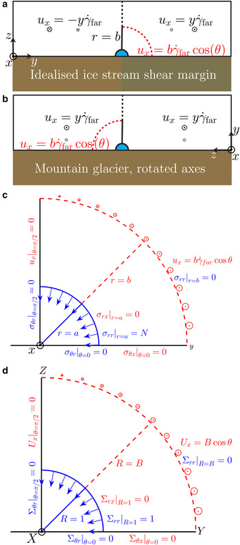
Fig. 2. Schematic representation for the quarter model domain shown in (a) an idealised ice stream shear margin and (b) a mountain glacier that has been rotated to translate vertical shear to lateral shear. These map to the physical space and boundary conditions for in-plane (blue) and antiplane (red) motion around a channel: (c) dimensionally and (d) non-dimensionally. In-plane motion occurs in the y–z plane and antiplane motion occurs in the x-direction. The coordinates are in a translating reference frame moving at $ - y{\dot \gamma _{{\rm far}}}$
, so that the system is antisymmetric about the z-axis.
$ - y{\dot \gamma _{{\rm far}}}$
, so that the system is antisymmetric about the z-axis.
We model a single R-channel incised into the ice in an idealised ice-stream shear margin or mountain glacier. Several simplifications are made in this analysis. We consider a perfectly flat bed without protrusions, cavities or till deformation. For basal boundary conditions, we use stress-free conditions at the base of the ice stream and no slip conditions at the bed of the mountain glacier. We neglect connections to other subgacial drainage pathways outside the R-channel. Furthermore, we neglect sediment transport and erosion of the sediment beneath the R-channel, prohibiting the formation of Nye channels or canals. These simplifications allow us to focus on the effects of ice deformation on the closure of R-channels.
We treat the ice as a homogeneous fluid with a Glen's law rheology, i.e. Eqn (4). The effective stress and strain rates are given in polar coordinates as
 $${\tau _{\rm E}} = \sqrt {\displaystyle{1 \over 4}{{({\sigma _{rr}} - {\sigma _{\theta \theta}} )}^2} + \sigma _{\theta r}^2 + \sigma _{rx}^2 + \sigma _{\theta x}^2}, $$
 $${{\dot \varepsilon}_{\rm E}} = \sqrt {{\dot \varepsilon}_{rr}^2 + {\dot \varepsilon}_{\theta r}^2 + {\dot \varepsilon}_{rx}^2 + {\dot \varepsilon}_{\theta x}^2}.$$
Relating the deviatoric stress and strain rates using Eqn (4), we write the strain rates in cylindrical polar coordinates as
 $${{\dot \varepsilon}_{rr}} = \displaystyle{{\partial {u_{\rm r}}} \over {\partial r}} = \displaystyle{1 \over 2}A\tau_{\rm E}^{n - 1} ({\sigma _{rr}} - {\sigma_{\theta \theta}} ),$$
 $${{\dot \varepsilon}_{\theta \theta}} = \displaystyle{1 \over r}\displaystyle{{\partial {u_\theta}} \over {\partial \theta}} + \displaystyle{{{u_{\rm r}}} \over r} = \displaystyle{1 \over 2}A\tau _{\rm E}^{n - 1} ({\sigma _{\theta \theta}} - {\sigma _{rr}}),$$
 $${{\dot \varepsilon}_{\theta r}} = \displaystyle{1 \over 2}\left( {\displaystyle{1 \over r}\displaystyle{{\partial {u_{\rm r}}} \over {\partial \theta}} + \displaystyle{{\partial {u_\theta}} \over {\partial r}} - \displaystyle{{{u_\theta}} \over r}} \right) = A\tau _{\rm E}^{n - 1} {\sigma _{\theta r}},$$
 $${{\dot \varepsilon}_{rx}} = \displaystyle{1 \over 2}\displaystyle{{\partial {u_x}} \over {\partial r}} = A\tau _{\rm E}^{n - 1} {\sigma _{rx}},$$
 $${{\dot \varepsilon}_{\theta x}} = \displaystyle{1 \over {2r}}\displaystyle{{\partial {u_x}} \over {\partial \theta}} = A\tau _{\rm E}^{n - 1} {\sigma _{\theta x}},$$
where ${{\dot \varepsilon}_{xx}} = 0$
due to the plane strain constraint, and
${{\dot \varepsilon}_{xx}} = 0$
due to the plane strain constraint, and ${{\dot \varepsilon}_{rr}} + {{\dot \varepsilon}_{\theta \theta}} = 0$
due to the mass conservation.
${{\dot \varepsilon}_{rr}} + {{\dot \varepsilon}_{\theta \theta}} = 0$
due to the mass conservation.
Rather than using an infinite domain (e.g. Nye, Reference Nye1953), we follow Evatt (Reference Evatt2015) and consider a finite domain that runs from $r = \sqrt {{y^2} + {z^2}} = a$
to r = b as shown in Figure 2. We do this for two reasons, firstly, it is more general and, secondly, the addition of antiplane shear can dominate in-plane motion in the far-field if the domain is too large. On the outer boundary of the finite domain, the normal stress is equal to the overburden (hydrostatic) pressure of the ice, ρ
ice
gH(1 − z/H), where H is the glacier thickness (Nye, Reference Nye1953; Evatt, Reference Evatt2015). Assuming that b/H ≪ 1 and therefore, that the overburden stress is nearly constant around the domain, we write the constant compressive overburden stress as σ
o = ρ
ice
gH. On the boundary of the channel, the normal stress is the water pressure inside the channel, p
w (<σ
o) following Spring and Hutter (Reference Spring and Hutter1981). Due to incompressibility and the pressure independence of the assumed rheology, we can add to our stress field the uniform tensile stress σ
o
δ
ij
, which has no effect on the flow field and removes any traction on the outer wall. This gives σ
rr
(r = a) = σ
o − p
w = N at the channel wall. Thus, the in-plane boundary conditions are
$r = \sqrt {{y^2} + {z^2}} = a$
to r = b as shown in Figure 2. We do this for two reasons, firstly, it is more general and, secondly, the addition of antiplane shear can dominate in-plane motion in the far-field if the domain is too large. On the outer boundary of the finite domain, the normal stress is equal to the overburden (hydrostatic) pressure of the ice, ρ
ice
gH(1 − z/H), where H is the glacier thickness (Nye, Reference Nye1953; Evatt, Reference Evatt2015). Assuming that b/H ≪ 1 and therefore, that the overburden stress is nearly constant around the domain, we write the constant compressive overburden stress as σ
o = ρ
ice
gH. On the boundary of the channel, the normal stress is the water pressure inside the channel, p
w (<σ
o) following Spring and Hutter (Reference Spring and Hutter1981). Due to incompressibility and the pressure independence of the assumed rheology, we can add to our stress field the uniform tensile stress σ
o
δ
ij
, which has no effect on the flow field and removes any traction on the outer wall. This gives σ
rr
(r = a) = σ
o − p
w = N at the channel wall. Thus, the in-plane boundary conditions are
 $${\sigma _{rr}}(r = a) = {\sigma _{\rm o}} - {\,p_{\rm w}} = N,\quad {\sigma _{rr}}(r = b) = 0.$$
In the antiplane direction, the shear stress on the inner channel is zero. On the outer boundary, we impose an antiplane velocity u x that varies linearly with distance y = bcos(θ) to represent far-field shearing. In this way, we write the antiplane boundary conditions as
 $${\sigma _{rx}}(r = a) = 0,\quad {u_x}(r = b) = {\dot \gamma _{{\rm far}}}b\cos (\theta ).$$
In order to isolate the effects of antiplane shear generated by differential velocity within the ice, we apply the following boundary conditions along the base of the glacier or idealised ice-stream shear margin,
 $${\sigma _{\theta r}}(r;\;\theta = 0) = 0,\quad {\sigma _{\theta x}}(r;\;\theta = 0) = 0.$$
In a mountain glacier with rotated axes, these boundary conditions represent symmetry conditions (Fig. 2b). In the idealised ice-stream shear margin, however, these boundary conditions represent how the basal ice interacts with the till. We assume that the till deforms plastically (Kamb, Reference Kamb1991; Tulaczyk and others, Reference Tulaczyk, Kamb and Engelhardt2000; Cuffey and Paterson, Reference Cuffey and Paterson2010) and σ
θx
(θ = 0) ≡ σ
zx
(z = 0) = τ
b, where τ
b is the basal shear stress supported by the till and less than or equal to the plastic yield stress of the till τ
y. If the basal shear stress τ
b is small compared with a characteristic antiplane shear stress within the ice τ
far, then the assumption σ
θx
(r; θ = 0) ≈ 0 is well justified (Schoof, Reference Schoof2012). In recent numerical simulations, Perol and others (Reference Perol, Rice, Platt and Suckale2015) find a basal shear stress of τ
b ≈ 60 − 75 kPa near an R-channel in an ice-stream shear margin. If we estimate the characteristic antiplane shear stress as ${\tau _{{\rm far}}} = ({\dot \gamma _{{\rm far}}}/2A{)^{1/n}} \approx 75$
kPa, using
${\tau _{{\rm far}}} = ({\dot \gamma _{{\rm far}}}/2A{)^{1/n}} \approx 75$
kPa, using ${\dot \gamma _{{\rm far}}} = 2 \times {10^{ - 9}}$
s−1 and A = 2.18 × 10⁻²⁴ Pa−n
s−1 (cf. Fig. 3; Table 1), we find that τ
far and σ
xz
from the simulations by Perol and others (Reference Perol, Rice, Platt and Suckale2015) are of similar magnitude. Thus, near the channel σ
θx
(r; θ = 0) ≈ 0 is potentially a poor approximation to the subglacial hydrology influenced basal boundary conditions prescribed by Perol and others (Reference Perol, Rice, Platt and Suckale2015). Furthermore, including in-plane traction along the ice/till interface, i.e. σ
θr
(r; θ = 0) = τ
b, would inhibit channel closure at the base (Weertman, Reference Weertman1972). It is likely all the same that this is a small effect due to the small channel closure velocities. Nevertheless, our goal is to isolate the effects of antiplane shear within the ice and therefore, we neglect antiplane and in-plane basal shear (Hutter and Olunloyo, Reference Hutter and Olunloyo1980; Barcilon and Macayeal, Reference Barcilon and Macayeal1993; Haseloff and others, Reference Haseloff, Schoof and Gagliardini2015). These channels can also be thought of as fully circular englacial channels, as the conditions σ
θx
(r; θ = 0) = 0 and σ
θr
(r; θ = 0) = 0 enforce symmetry across the y-axis.
${\dot \gamma _{{\rm far}}} = 2 \times {10^{ - 9}}$
s−1 and A = 2.18 × 10⁻²⁴ Pa−n
s−1 (cf. Fig. 3; Table 1), we find that τ
far and σ
xz
from the simulations by Perol and others (Reference Perol, Rice, Platt and Suckale2015) are of similar magnitude. Thus, near the channel σ
θx
(r; θ = 0) ≈ 0 is potentially a poor approximation to the subglacial hydrology influenced basal boundary conditions prescribed by Perol and others (Reference Perol, Rice, Platt and Suckale2015). Furthermore, including in-plane traction along the ice/till interface, i.e. σ
θr
(r; θ = 0) = τ
b, would inhibit channel closure at the base (Weertman, Reference Weertman1972). It is likely all the same that this is a small effect due to the small channel closure velocities. Nevertheless, our goal is to isolate the effects of antiplane shear within the ice and therefore, we neglect antiplane and in-plane basal shear (Hutter and Olunloyo, Reference Hutter and Olunloyo1980; Barcilon and Macayeal, Reference Barcilon and Macayeal1993; Haseloff and others, Reference Haseloff, Schoof and Gagliardini2015). These channels can also be thought of as fully circular englacial channels, as the conditions σ
θx
(r; θ = 0) = 0 and σ
θr
(r; θ = 0) = 0 enforce symmetry across the y-axis.

Fig. 3. Velocity data for computing the magnitude of the antiplane strain rate ${\dot \gamma _{{\rm far}}}$
: (a) Ice velocity with depth for Worthington Glacier, Alaska from Harper and others (Reference Harper2001). (b) Ice stream shear margin surface velocity data between stations S17 and UpB on the Upper Whillans Ice Stream, Siple Coast, West Antarctica from January 1994 to January 1995 (Echelmeyer and Harrison, Reference Echelmeyer and Harrison1999; Truffer and Echelmeyer, Reference Truffer and Echelmeyer2003, Reference Truffer and Echelmeyer2005). The green circles indicate the portion of the shear zone used to calculate the slope shown in the figure.
${\dot \gamma _{{\rm far}}}$
: (a) Ice velocity with depth for Worthington Glacier, Alaska from Harper and others (Reference Harper2001). (b) Ice stream shear margin surface velocity data between stations S17 and UpB on the Upper Whillans Ice Stream, Siple Coast, West Antarctica from January 1994 to January 1995 (Echelmeyer and Harrison, Reference Echelmeyer and Harrison1999; Truffer and Echelmeyer, Reference Truffer and Echelmeyer2003, Reference Truffer and Echelmeyer2005). The green circles indicate the portion of the shear zone used to calculate the slope shown in the figure.
Along the vertical axis of the quarter circle domain we apply the boundary conditions:
 $${\sigma _{\theta r}}(r;\;\theta = \pi /2) = 0,\quad {u_x}(r;\;\theta = \pi /2) = 0.$$
These represent symmetry and antisymmetry conditions and are consistent with the boundary conditions applied at the outer edge. For the mountain glacier with rotated axes, the condition u x = 0 amounts to a no slip boundary condition at the base, which is an approximation unless the base is frozen to the bed or pore pressure is depressed in the basal till (Hindmarsh, Reference Hindmarsh2004; Cuffey and Paterson, Reference Cuffey and Paterson2010).
Scaling all lengths by the channel radius a, we have r = aR and the dimensionless outer radius B = b/a, which defines the domain size. We scale the antiplane shear strain rate by ${\dot \gamma _{{\rm far}}}$
and the in-plane components of strain rate by AN
n
, which is the dimensional scaling of the Nye strain rate, so that
${\dot \gamma _{{\rm far}}}$
and the in-plane components of strain rate by AN
n
, which is the dimensional scaling of the Nye strain rate, so that ${{\dot \varepsilon}_{rr}} = A{N^n}{\dot E_{rr}}$
. A consequence of this scaling is that the strain rates will not necessarily be close to unity: at the edge of the channel
${{\dot \varepsilon}_{rr}} = A{N^n}{\dot E_{rr}}$
. A consequence of this scaling is that the strain rates will not necessarily be close to unity: at the edge of the channel ${\dot E_{rr}} = {n^{ - n}}$
, which is 1/27 for n = 3. We can non-dimensionalise the effective strain rate in the same way as the in-plane strain rates, which gives
${\dot E_{rr}} = {n^{ - n}}$
, which is 1/27 for n = 3. We can non-dimensionalise the effective strain rate in the same way as the in-plane strain rates, which gives
 $${\dot E_{\rm E}} = \sqrt {\dot E_{rr}^{\rm 2} + \dot E_{\theta r}^2 + {S^2}\left( {\dot E_{rx}^2 + \dot E_{\theta x}^2} \right)}, $$
where S is the strain rate ratio of antiplane to in-plane strain rates
 $$S = \displaystyle{{{{\dot \gamma} _{{\rm far}}}} \over {A{N^n}}}.$$
This ratio represents the importance of the superimposed antiplane shear strain rate ${\dot \gamma _{{\rm far}}}$
, as compared with a characteristic in-plane strain rate AN
n
.
${\dot \gamma _{{\rm far}}}$
, as compared with a characteristic in-plane strain rate AN
n
.
The strain rate ratio S can also be written as:
 $$S = {n^{ - n}}\left( {\displaystyle{{{{\dot \gamma} _{{\rm far}}}} \over {\dot \varepsilon _{\theta \theta} ^{{\rm Nye}}}}} \right),$$
 $$= 2{\left( {\displaystyle{{{\tau _{{\rm far}}}} \over N}} \right)^n},$$
where we use
 $${\dot \varepsilon}_{\theta \theta}^{\rm Nye} = A{\left( {\displaystyle{N \over n}} \right)^n}\quad {\rm and}\quad {\tau _{{\rm far}}} = {\left( {\displaystyle{{{{\dot \gamma} _{{\rm far}}}} \over {2A}}} \right)^{1/n}}.$$
Thus, S represents the importance of the antiplane strain rate imposed on the outer edge of the domain to the in-plane creep closure of the channel.
Since the stress driving creep closure at the edge of the channel scales with N, we non-dimensionalise the in-plane stresses so that σ rr = NΣ rr . Following the above convention for the antiplane strain rates, we scale antiplane stresses by SN so that σ rx = SNΣ rx . We now write the effective stress as τ E = NT E, where
 $${T_{\rm E}} = \sqrt {\displaystyle{1 \over 4}{{({\Sigma _{rr}} - {\Sigma _{\theta \theta}} )}^2} + \Sigma _{\theta r}^2 + {S^2}\left( {\Sigma _{rx}^2 + \Sigma _{\theta x}^2} \right)}. $$
The velocities scale as the strain rates multiplied by the channel radius so that
 $${u_{\rm r}} = Aa{N^n}{U_{\rm r}}\quad {\rm and}\quad {u_x} = Aa{N^n}S{U_x}.$$
The equations for mass and momentum conservation now become
 $$\displaystyle{1 \over R}\displaystyle{\partial \over {\partial R}}(R{\Sigma _{rr}}) + \displaystyle{1 \over R}\displaystyle{{\partial {\Sigma _{\theta r}}} \over {\partial \theta}} - \displaystyle{{{\Sigma _{\theta \theta}}} \over R} = 0,$$
 $$\displaystyle{1 \over R}\displaystyle{\partial \over {\partial R}}(R{\Sigma _{\theta r}}) + \displaystyle{1 \over R}\displaystyle{{\partial {\Sigma _{\theta \theta}}} \over {\partial \theta}} + \displaystyle{{{\Sigma _{\theta r}}} \over R} = 0,$$
 $$\displaystyle{1 \over R}\displaystyle{\partial \over {\partial R}}(R{\Sigma _{rx}}) + \displaystyle{1 \over R}\displaystyle{{\partial {\Sigma _{\theta x}}} \over {\partial \theta}} = 0,$$
 $${\dot E_{rr}} + {\dot E_{\theta \theta}} = \displaystyle{{{\rm d}{U_{\rm r}}} \over {{\rm d}R}} + \displaystyle{{{U_{\rm r}}} \over R} + \displaystyle{1 \over R}\displaystyle{{\partial {U_\theta}} \over {\partial \theta}} = 0.$$
The boundary conditions, in non-dimensional form (Fig. 2d), are then
 $${\Sigma _{rr}}(R = 1) = 1,\quad {\Sigma _{rr}}(R = B) = 0,$$
 $${\Sigma _{rx}}(R = 1) = 0,\quad {U_x}(R = B) = B\cos (\theta ),$$
 $${\Sigma _{\theta r}}(R;\;\theta = 0) = 0,\quad {\Sigma _{\theta x}}(R;\;\theta = 0) = 0,$$
 $${\Sigma _{\theta r}}(R;\;\theta = \pi /2) = 0,\quad {U_x}(R;\;\theta = \pi /2) = 0.$$
2.1. Reasonable strain rate ratio values
Here we estimate the size of the antiplane strain rate ${\dot \gamma _{{\rm far}}}$
using data from the the Worthington Glacier, Alaska (Harper and others, Reference Harper2001), which is shown in Figure 3a, and the Upper Whillans Ice Stream shear margin surface velocity data shown in Figure 3b (Echelmeyer and Harrison, Reference Echelmeyer and Harrison1999; Truffer and Echelmeyer, Reference Truffer and Echelmeyer2003, Reference Truffer and Echelmeyer2005). These data give the estimates of
${\dot \gamma _{{\rm far}}}$
using data from the the Worthington Glacier, Alaska (Harper and others, Reference Harper2001), which is shown in Figure 3a, and the Upper Whillans Ice Stream shear margin surface velocity data shown in Figure 3b (Echelmeyer and Harrison, Reference Echelmeyer and Harrison1999; Truffer and Echelmeyer, Reference Truffer and Echelmeyer2003, Reference Truffer and Echelmeyer2005). These data give the estimates of ${\dot \gamma _{{\rm far}}} = 2 \times {10^{ - 8}}$
s−1 for mountain glaciers and
${\dot \gamma _{{\rm far}}} = 2 \times {10^{ - 8}}$
s−1 for mountain glaciers and ${\dot \gamma _{{\rm far}}} = 4 \times {10^{ - 9}}$
s−1 for ice-stream shear margins. We then combine the value for the antiplane strain rate
${\dot \gamma _{{\rm far}}} = 4 \times {10^{ - 9}}$
s−1 for ice-stream shear margins. We then combine the value for the antiplane strain rate ${\dot \gamma _{{\rm far}}}$
with a representative value for the effective pressure N to compute the strain rate ratio
${\dot \gamma _{{\rm far}}}$
with a representative value for the effective pressure N to compute the strain rate ratio $S = {\dot \gamma _{{\rm far}}}/A{N^n}$
. We also note that the actual value can vary quite significantly, leading to changes in the value of S. The ranges of S we find for reasonable parameter values are S ~ 10−4–10−2 for mountain glaciers and S ~ 10−3–10−1 for ice-stream shear margins. These ranges serve as guidelines for what values of S are relevant to channels in antiplane shear, as in how channel size and shape might vary with S.
$S = {\dot \gamma _{{\rm far}}}/A{N^n}$
. We also note that the actual value can vary quite significantly, leading to changes in the value of S. The ranges of S we find for reasonable parameter values are S ~ 10−4–10−2 for mountain glaciers and S ~ 10−3–10−1 for ice-stream shear margins. These ranges serve as guidelines for what values of S are relevant to channels in antiplane shear, as in how channel size and shape might vary with S.
2.1.1. Mountain glaciers
We estimate the strain rate ratio S as
 $$S{\rm \sim} \displaystyle{u \over {Ah{N^n}}},$$
where u and h are the velocity difference and height of basal shear (Fig. 3a). For example, data from Harper and others (Reference Harper2001) and Bartholomaus and others (Reference Bartholomaus, Anderson and Anderson2011) as well as Cuffey and Paterson (Reference Cuffey and Paterson2010), suggest the estimates
 $$\eqalign{& u \approx 21\;{\rm m}\;{{\rm a}^{ - 1}},\;A \approx 2.4 \times {10^{ - 24}}\;{{\rm s}^{ - 1}}\;{\rm P}{{\rm a}^{ - n}}, \cr & h \approx 33\;{\rm m}\quad {\rm and}\quad N \approx 1.35 \times {10^6}\;{\rm Pa}.} $$
The effective pressure is similar to the values reported by Kavanaugh and Clarke (Reference Kavanaugh and Clarke2000), Flowers and Clarke (Reference Flowers and Clarke2002b) and Schoof and others (Reference Schoof, Rada, Wilson, Flowers and Haseloff2014). Combining these estimates we find a strain rate ratio of
 $$S \approx {10^{ - 3}}.$$
By varying the parameters slightly we find a representative range of S ~ 10−4–10−2.
2.1.2. Ice-stream shear margins
The scaling for the strain rate ratio in ice-stream shear margins is similar to the scaling for mountain glaciers except that the length scale L is now the width of the shear margin (Fig. 3b), so that
 $$S{\rm \sim} \displaystyle{{{u_{\rm s}}} \over {AL{N^n}}}.$$
The velocity profile in the ice stream and its shear margin are approximately uniform with depth allowing us to use the measured surface velocity u s to describe the flow at the base (Kamb, Reference Kamb, Alley and Bindschadler2001). Using the data from Echelmeyer and Harrison (Reference Echelmeyer and Harrison1999), Joughin and Tulaczyk (Reference Joughin and Tulaczyk2002), as well as Cuffey and Paterson (Reference Cuffey and Paterson2010), we choose the parameters
 $$\eqalign{& {u_{\rm s}} \approx 320\;{\rm m}\;{{\rm a}^{ - 1}},\;A \approx 2.18 \times {10^{ - 24}}\;{{\rm s}^{ - 1}}\;{\rm P}{{\rm a}^{ - n}}, \cr & L \approx 2500\;{\rm m}\quad {\rm and}\quad N \approx 5 \times {10^5}\;{\rm Pa}.} $$
Since R-channels operate at lower water pressure (larger effective pressure) than water flow through linked cavities or sediments, the value for the effective pressure used here is larger than found by Blankenship and others (Reference Blankenship, Bentley, Rooney and Alley1987) for the water-saturated subglacial till under Ice Stream B (Whillans Ice Stream). Moreover, the water pressure beneath the ice streams is still closer to the overburden pressure than in mountain glaciers (Engelhardt and Kamb, Reference Engelhardt and Kamb1997, Reference Engelhardt and Kamb1998; Tulaczyk and others, Reference Tulaczyk, Kamb and Engelhardt2001). These parameters lead to strain rate ratio of about
 $$S \approx {10^{ - 2}},$$
which varies in the range S ~ 10−3–10−1 for slightly different parameter values.
3. ANALYSIS
The estimates for S from mountain glaciers and ice streams show that it is a small quantity. In this limit of small antiplane shear, we are able to derive a closed-form solution for the antiplane velocity, which allows us to benchmark the combined in-plane and antiplane finite element code that is used for later calculations. After examining the small S limit, we then turn to the opposite limit, when antiplane motion dominates, and find a scaling for the creep closure as a function of S. The reader who is primarily interested in how the R-channel diameter scales with S and non-circular R-channels can skip to the next section.
For our numerical solutions, we use the existing numerical finite-element method (FEM) package ABAQUS (Dassault Systémes, 2012). To model the fully coupled problems, where the ice viscosity is a function of both the in-plane and the antiplane components, we construct a single-element thick, three-dimensional FEM model constrained to deform by a combination of plane strain and antiplane strain. We couple the displacements of the nodes on opposite faces to ensure that the model maintains a state of combined antiplane and plane strain. We generate the FEM using isoparametric elements with significant refinement near the channel boundary. We compare numerical solutions to the known in-plane Nye solution without antiplane shearing and find a nodal error of <0.8%.
3.1. Small antiplane velocity benchmark
Here, we show that when S is very small we can derive an analytical solution for the antiplane velocity. The reason for considering this limit is that when the applied antiplane shear is sufficiently small, the in-plane motion dominates throughout the domain and sets the viscosity of the ice. Thus, the creep closure of the R-channel is given by the Nye solution. Evatt (Reference Evatt2015) gives a derivation for the finite domain Nye solution, which in the dimensionless variables used here is given as
 $${U_r} = - \displaystyle{{{n^{ - n}}} \over R}\displaystyle{{{B^2}} \over {{{({B^{2/n}} - 1)}^n}}}.$$
In this limit, the effective deviatoric stress is only a function of R and given as
 $${T_{\rm E}} = \displaystyle{1 \over 2}({\Sigma _{rr}} - {\Sigma _{\theta \theta}} ) = \displaystyle{1 \over {n{R^{2/n}}}}{\left( {1 - \displaystyle{1 \over {{B^{2/n}}}}} \right)^{ - 1}}.$$
Using Eqns (14) and (15), we can insert the effective stress into the in-plane force balance, Eqn (20), and find
 $${R^{(2/n) - 1}}\displaystyle{\partial \over {\partial R}}\left( {{R^{3 - (2/n)}}\displaystyle{{\partial {U_x}} \over {\partial R}}} \right) + \displaystyle{{{\partial ^2}{U_x}} \over {\partial {\theta ^2}}} = 0.$$
This is an equidimensional, linear equation for the antiplane velocity u x . The antiplane boundary conditions are
 $${\left. {\displaystyle{{\partial {U_x}} \over {\partial \theta}}} \right \vert _{\theta = 0}} = 0, {\left. {\displaystyle{{\partial {U_x}} \over {\partial R}}} \right \vert _{R = 1}} = 0\quad {\rm and}\quad {U_x}(R = B) = B\cos (\theta ).$$
A method to solve Eqn (25) subject to these boundary conditions is described in Appendix A. The solution for the antiplane velocity u x is
 $${U_x} = B\displaystyle{{({R^{{\lambda _ +}}} /{\lambda _ +} ) - ({R^{{\lambda _ -}}} /{\lambda _ -} )} \over {({B^{{\lambda _ +}}} /{\lambda _ +} ) - ({B^{{\lambda _ -}}} /{\lambda _ -} )}}\cos (\theta ),$$
where λ
+ and λ
− are positive and negative solutions to the characteristic polynomial, Eqn (A1) for k = 1. Equation (26) also shows that points at the edge of the channel displace in the antiplane direction as if the interior underwent a homogeneous deformation rate and therefore, similar to an Eshelby (Reference Eshelby1957) inclusion in a composite solid. Figure 4 shows the numerical strain rate $\dot \Gamma _{xy}^N $
computed from the full ABAQUS simulation with S = 10−4. The error between
$\dot \Gamma _{xy}^N $
computed from the full ABAQUS simulation with S = 10−4. The error between $\dot \Gamma _{xy}^N $
and the derivative of Eqn (26), ∂U
x
/∂Y is <0.1% and serves as a good benchmark for the ABAQUS simulations.
$\dot \Gamma _{xy}^N $
and the derivative of Eqn (26), ∂U
x
/∂Y is <0.1% and serves as a good benchmark for the ABAQUS simulations.

Fig. 4. Horizontal antiplane strain rate ∂U
x
/∂Y for S ≪ 1, small antiplane perturbation of in-plane flow field: ABAQUS numerical solution $\dot \Gamma _{xy}^N $
to the full problem with S = 10−4. The maximum value of horizontal strain rate is <0.1% from the analytical solution of 3.7472 as calculated from the derivative of Eqn (26) and is located on the top of the channel.
$\dot \Gamma _{xy}^N $
to the full problem with S = 10−4. The maximum value of horizontal strain rate is <0.1% from the analytical solution of 3.7472 as calculated from the derivative of Eqn (26) and is located on the top of the channel.
3.2. Region of validity
We now consider under what conditions the analytical solution for the antiplane velocity is valid. From the Nye solution, Eqn (24), we can see that the in-plane velocity decays as 1/R. The antiplane velocity, however, is largest along the outer edge. Thus, for the perturbation solution to be valid throughout the domain, we require that the ratio of antiplane shear strain rate to the minimum in-plane strain rate is small, i.e.
 $$\displaystyle{{{{\dot \gamma} _{{\rm far}}}} \over {{{\dot \varepsilon} _{rr}}(R = B)}} = {n^n}S{({B^{2/n}} - 1)^n}{\rm \ll} 1.$$
We can rearrange the right-hand side to find the critical non-dimensional radius
 $${B_{{\rm cr}}} = {\left( {1 + \displaystyle{1 \over {n{S^{1/n}}}}} \right)^{n/2}}.$$
Thus, the outer radius must satisfy the inequality B ≪ B cr in order for the entire domain to be dominated by in-plane creep closure. This condition states that the domain size must decrease as S increases. For S = 10−3 and n = 3, we have that B cr = 10 and, thus for B = 10, this inequality is violated as S approaches 10−3 but not unity as one might initially expect.
If the size of the domain is much larger than B
cr, the perturbation solution is no longer valid near the boundary and there is a transition to a region that is antiplane dominated (Weertman, Reference Weertman1972). The small S scaling of Eqn (27) predicts that the transition will occur at a radius $R{\rm \sim} 1/\sqrt S $
, as this is when
$R{\rm \sim} 1/\sqrt S $
, as this is when ${\dot E_{rr}}{\rm \sim} S$
. Close to the channel, the dominant flow of ice is inward creep closure of the channel. In the far field, ice predominantly flows downstream. The transition radius,
${\dot E_{rr}}{\rm \sim} S$
. Close to the channel, the dominant flow of ice is inward creep closure of the channel. In the far field, ice predominantly flows downstream. The transition radius, $R{\rm \sim} 1/\sqrt S $
, represents the crossover between the inward creep closure dominated flow and the antiplane flow downstream.
$R{\rm \sim} 1/\sqrt S $
, represents the crossover between the inward creep closure dominated flow and the antiplane flow downstream.
3.3. Limit of large antiplane velocity
Here we consider very large values of S, when antiplane shear strain rate strongly dominates the in-plane strain rate. In this limit, the non-dimensional effective stress and strain rate, from Eqns (9) and (10), reduce to
 $${T_{\rm E}} = S\sqrt {\Sigma _{rx}^2 + \Sigma _{\theta x}^2} \quad {\rm and}\quad {\dot E_{\rm E}} = S\sqrt {\dot E_{rx}^2 + \dot E_{\theta x}^2}. $$
Thus, the effective viscosity of the ice is set by the antiplane motion. In this regime, the non-linearity of the equations in the in-plane direction disappears and the channel will close like a Newtonian (n = 1) fluid with a spatially variable viscosity, much like the observations of Haefeli (Reference Haefeli1951) and Glen (Reference Glen1956). Here we seek to determine how the creep closure velocity U r depends on S.
To start, we use quantities that are averaged over θ ∈ [0, π] and consider deviations from axisymmetric creep closure in a later section. Mass conservation can then be written as
 $$\displaystyle{{\partial {{\overline U} _r}} \over {\partial R}} + \displaystyle{{{{\overline U} _r}} \over R} = 0,$$
where any U
θ
dependence integrates out, and we can write the solution ${\overline U _r}$
in the form,
${\overline U _r}$
in the form,
 $${\overline U _r} = - \displaystyle{C \over R}.$$
Now in the large S limit, the in-plane rheology is given as
 $${\dot E_{rr}} = \displaystyle{1 \over 2}{S^{(n - 1)/n}}{\left( {\dot E_{rx}^2 + \dot E_{\theta x}^2} \right)^{(n - 1)/(2n)}}({\Sigma _{rr}} - {\Sigma _{\theta \theta}} ).$$
Along the channel, the radial stress and hoop stress scale as
 $${\Sigma _{rr}} - {\Sigma _{\theta \theta}} {\rm \sim} f\,(n,\;B)$$
from the boundary conditions, where Σ
rr
= 1 and Σ
θθ
is independent of S and an unknown function of n and B. The radial antiplane strain rate ${\dot E_{rx}}$
along the hole is zero and therefore we are left with
${\dot E_{rx}}$
along the hole is zero and therefore we are left with
 $${\overline E _{rr}}{\rm \sim} {S^{n - 1/n}}\dot E_{\theta x}^{n - 1/n} f\,(n,\;B).$$
The average in-plane strain rate scales with the in-plane velocity as
 $${\overline E _{rr}}{\rm \sim} - {\overline E _{\theta \theta}} {\rm \sim} - \displaystyle{{{{\overline U} _r}} \over R},$$
and inserting the strain rate scaling at R = 1 gives
 $$\left \vert {{{\overline U} _r}} \right \vert {\rm \sim} {S^{(n - 1)/n}},$$
which can be seen in Figure 5 for three different values of n and B = 10.

Fig. 5. Large S scaling for the average creep closure $\left\vert {{{\overline U} _{\rm r}}} \right\vert $
at R = 1. Black circles are ABAQUS simulation results (linear spacing in S) and black lines follow scaling with a best-fit coefficient of proportionality. The outer radius for these simulations is B = 10.
$\left\vert {{{\overline U} _{\rm r}}} \right\vert $
at R = 1. Black circles are ABAQUS simulation results (linear spacing in S) and black lines follow scaling with a best-fit coefficient of proportionality. The outer radius for these simulations is B = 10.
4. R-CHANNEL DIAMETER WITH S
In the previous two sections, we examined the creep closure velocity in the limits of small and large antiplane strain rate. Here we show the influence of antiplane shear on the size of R-channels. For the small antiplane shear case, e.g. S ≪ 1, there is no change to the standard Röthlisberger analysis and we can insert the parameters from Table 1 into Eqn (8) and find that
 $${D_{{\rm Nye}}} = {\left( {\displaystyle{{{2^{7/3}}{{(1 + 2/\pi )}^{2/3}}{\rho _{{\rm ice}}}{\rm {\cal L}}} \over {{n^n}{\rho _{\rm w}}g}}\displaystyle{{A{N^n}{n_{\rm m}}} \over {\mathop {\sin} \nolimits^{3/2}(\alpha )}}} \right)^{3/2}} \approx 2.3\;{\rm m}.$$
This is consistent with Vogel and others (Reference Vogel2005), who show flowing water with a depth of 1.6 m at the base of the dormant Kamb ice-stream shear margin.
For arbitrary S, we turn to numerical simulations to determine the average creep closure velocity ${\bar u_{{\rm cr}}}$
as a function of the applied antiplane strain rate
${\bar u_{{\rm cr}}}$
as a function of the applied antiplane strain rate ${\dot \gamma _{{\rm far}}}$
and a fixed effective pressure N. Figure 6 shows that for
${\dot \gamma _{{\rm far}}}$
and a fixed effective pressure N. Figure 6 shows that for $S{\rm \lesssim} {10^{ - 3}}$
, the Nye solution holds and the predicted channel size is exactly that found above. As S increases, it leaves the small perturbation range and we find that for S ~ 10−2, the diameter roughly doubles in size. For very large S, we can use the scaling from the last section to show that the diameter of the channel should scale as
$S{\rm \lesssim} {10^{ - 3}}$
, the Nye solution holds and the predicted channel size is exactly that found above. As S increases, it leaves the small perturbation range and we find that for S ~ 10−2, the diameter roughly doubles in size. For very large S, we can use the scaling from the last section to show that the diameter of the channel should scale as $D {\rm \sim} {S^{3(n - 1)/(2n)}}$
. As S increases the R-channel size increases, which can be seen from Eqn (7): for a constant N, if
$D {\rm \sim} {S^{3(n - 1)/(2n)}}$
. As S increases the R-channel size increases, which can be seen from Eqn (7): for a constant N, if ${\bar u_{{\rm cr}}}$
increases then D must also increase. A larger diameter also implies larger discharge Q and therefore, sufficient available water is required for the channel shape to increase at constant effective pressure.
${\bar u_{{\rm cr}}}$
increases then D must also increase. A larger diameter also implies larger discharge Q and therefore, sufficient available water is required for the channel shape to increase at constant effective pressure.

Fig. 6. R-channel diameter as a function of the antiplane to in-plane strain rate ratio S. Representative ranges of S for ice streams and mountain glaciers are based estimates from data (Echelmeyer and Harrison, Reference Echelmeyer and Harrison1999; Harper and others, Reference Harper2001; Truffer and Echelmeyer, Reference Truffer and Echelmeyer2005). Error bars denote RMS deviations from axisymmetry.
If the channel pressure is allowed to vary, our results indicate that adding in antiplane shear allows channels at a given diameter (or flow rate) to operate at higher water pressures (lower effective pressure). For an R-channel with a fixed diameter, the flow rate through the channel is fixed by Eqn (5), and the creep closure rate of the channel is then fixed by Eqn (6). Our results in Figure 5 show that the creep closure velocity increases with $S = {\dot \gamma _{{\rm far}}}/(A{N^n})$
. Thus, to maintain a fixed creep closure rate with a fixed far-field strain rate
$S = {\dot \gamma _{{\rm far}}}/(A{N^n})$
. Thus, to maintain a fixed creep closure rate with a fixed far-field strain rate ${\dot \gamma _{{\rm far}}}$
, the channel pressure must increase, leading to a lower effective pressure and a reduction in the strength of the bed.
${\dot \gamma _{{\rm far}}}$
, the channel pressure must increase, leading to a lower effective pressure and a reduction in the strength of the bed.
5. DISCUSSION
Here we discuss implications of increasing antiplane shear around R-channels to subglacial hydrology and extend our analysis to determine non-circular R-channel shapes. In Figure 6, we show the average R-channel diameter as a function of the strain rate ratio S, assuming a semicircular channel. Our numerical simulations do, however, allow for analysis of the expected shape and how the deviations from circular vary with applied antiplane shear. After discussing non-circular R-channels, we describe how our results for the diameter of an R-channel in regions of antiplane shear might influence subglacial hydrology and glacier sliding. We discuss the implications of these results to surging glaciers and describe how the transition between channelised drainage and linked-cavity systems may be facilitated by including shear in the R-channel analysis. Finally, we examine the relationship between the outer boundary of the domain and the applied antiplane shear and its implications for subglacial hydrology.
5.1. Non-circular R-channels
There is a small but growing literature on non-circular R-channels. Hooke and others (Reference Hooke, Laumann and Kohler1990) consider channel cross sections given by the space between the arc of a circle and its chord and find better agreement with water pressure data from Austdalsbreen and Storglaciären than standard semicircular R-channels. Fowler and Ng (Reference Fowler and Ng1996) model low, broad canals in sediments during jökulhlaups. In their model, the height of the channel is governed by the creep closure of ice and the width of the channel is determined by erosion of the sediments. This method provides more reasonable values for the Manning roughness coefficient and yields an improved simulation of the 1972 Grímsvötn jökulhlaup. Cutler (Reference Cutler1998) uses a finite element model to determine the seasonal evolution of an R-channel cross section and examine the effects of variable water input. He finds that all channels tend toward low, broad shapes. Furthermore, for two channels with equivalent areas, the channel with a lower width-to-height ratio (i.e. more circular) will expand faster, stealing water from neighbouring channels. More recently, Dallaston and Hewitt (Reference Dallaston and Hewitt2014) study the stability of R-channels under coupled interfacial melting and creep closure. They show that circular channels under axisymmetric in-plane loading with a constant melt rate are unstable to linear perturbations for both shear-thinning and Newtonian viscosities. Moreover, they show that this instability can be stabilised by the addition of a uniform heat source that diffuses to the free boundary of the channel.
We complement these studies by examining how antiplane shear modifies initially circular channels. To analyse the effect of shear on the shape of the channel, we break the creep closure into an average and fluctuating component, i.e.
 $${u_{\rm r}} = {\bar u_{{\rm cr}}} + {u^{\prime}_{\rm r}}.$$
Our previous analysis neglected ${u'_{\rm r}}/{\bar u_{{\rm cr}}}$
as a very small quantity. This assumption is reasonable because the maximum value of
${u'_{\rm r}}/{\bar u_{{\rm cr}}}$
as a very small quantity. This assumption is reasonable because the maximum value of ${u'_{\rm r}}/{\bar u_{{\rm cr}}}$
for S = 10−1 is 0.1. However, we wish to look at channels that deviate from circular. In keeping with the idea that
${u'_{\rm r}}/{\bar u_{{\rm cr}}}$
for S = 10−1 is 0.1. However, we wish to look at channels that deviate from circular. In keeping with the idea that ${u'_{\rm r}}/{\bar u_{{\rm cr}}}{\rm \ll} 1$
, we ignore small variations in diameter and derive Eqn (7) identically as before. We then insert u
r in the place of
${u'_{\rm r}}/{\bar u_{{\rm cr}}}{\rm \ll} 1$
, we ignore small variations in diameter and derive Eqn (7) identically as before. We then insert u
r in the place of ${\bar u_{{\rm cr}}}$
in Eqn (7), which gives approximately
${\bar u_{{\rm cr}}}$
in Eqn (7), which gives approximately
 $$D = 4{\left( {1 + \displaystyle{2 \over \pi}} \right)^{2/5}}{\left( {\displaystyle{{\rho_{\rm ice}{\cal L}} \over {\rho_{\rm w}g}}\displaystyle{{{\bar u}_{\rm cr}n_{\rm m}} \over {{\sin}^{3/2}(\alpha)}}}\right)^{3/5}}{\left[{1 + \displaystyle{3 \over 5}\displaystyle{{u^{\prime}_r} \over {{\bar u}_{\rm cr}}}}\right]}.$$
Inserting u′r, which is dependent on θ, from the simulations into Eqn (31), we plot the cross section of the channels for three values of S in Figure 7. We can see that the deviations from circular are not noticeable at S = 2 × 10⁻³ and it is not until S ≳ 10−2 that the deviations become significant. The extent to which the channels deviate from circular are plotted as error bars in Figure 6.

Fig. 7. Numerical prediction for the shape of R-channels as a function of S: The vertical shear present in mountain glaciers leads to short, broad channels that are wider than tall (cyan dot dashed curves) and the lateral shear in idealised ice stream shear margins leads to channels that are taller than wide (blue dashed curves). The azimuthally averaged velocity results in semicircular channels (black solid curves).
The channel shapes predicted by our simulations indicate that when the superimposed antiplane strain rate increases, the creep closure velocity increases on the top of the channel (i.e. along the z-axis of Fig. 2) and decreases on the sides (along y-axis) relative to the average creep closure velocity ${\bar u_{{\rm cr}}}$
. This makes sense, in light of Figure 4, where the antiplane strain rate concentrates on the top of the channel and since the viscosity is lower, the channel closes faster locally. Thus, using a melt rate proportional to the creep closure velocity (i.e. steady-state non-uniform melting), circular channels deform and melt into channels that are taller than they are wide. In mountain glaciers under vertical antiplane shear our simulations predict channels that are wider than tall, which is in agreement with the observations (e.g. Fountain, Reference Fountain1993; Hock and Hooke, Reference Hock and Hooke1993; Fountain and Walder, Reference Fountain and Walder1998). In idealised ice-stream shear margins, the antiplane shear straining is along the axis of the channel and our simulations indicate that channels that are taller than wide might form.
${\bar u_{{\rm cr}}}$
. This makes sense, in light of Figure 4, where the antiplane strain rate concentrates on the top of the channel and since the viscosity is lower, the channel closes faster locally. Thus, using a melt rate proportional to the creep closure velocity (i.e. steady-state non-uniform melting), circular channels deform and melt into channels that are taller than they are wide. In mountain glaciers under vertical antiplane shear our simulations predict channels that are wider than tall, which is in agreement with the observations (e.g. Fountain, Reference Fountain1993; Hock and Hooke, Reference Hock and Hooke1993; Fountain and Walder, Reference Fountain and Walder1998). In idealised ice-stream shear margins, the antiplane shear straining is along the axis of the channel and our simulations indicate that channels that are taller than wide might form.
5.2. Implications for subglacial hydrology
In models of subglacial hydrology, the downstream ice velocity typically is ignored in the creep closure of the R-channels. Here we find that for low ice flow velocities, it is reasonable to neglect the effect of shear on the channel size, but in regions of high-velocity gradients, the channel size can increase significantly for a fixed pressure difference. This equivalently implies that for a fixed volume flux of water (or equivalently R-channel diameter), the channel will operate at a higher water pressure (lower effective pressure). Therefore, decreasing the effective pressure by accounting for antiplane shear, can increase the basal sliding velocity for a constant basal shear stress.
By including the feedback between antiplane shear and effective pressure, the transition between channelised and distributed drainage occurs at a lower effective pressure and a switch between the two styles of drainage may be facilitated. For hydrologically controlled surging glaciers, systems of channels can coexist with distributed drainage networks (Fowler, Reference Fowler1987, Reference Fowler1989, Reference Fowler2011). If the flux of water in the system increases slightly, then the effective pressure in the distributed network increases but decreases in the channels. The channelised portion of the hydrologic system can be unstable. As the flow rate increases, if the effective pressure in the channels decreases more than the distributed drainage effective pressure, then the drainage through channels can shut off. This mechanism leaves only a distributed drainage network that favours sliding. Traditionally, the basal sliding velocity u b is related to the effective pressure in the distributed network via Eqn (1), and therefore, there is a transition from channels to distributed drainage when S Λ = u b/(AHN n ) reaches a critical value. This relationship can then be inserted into Eqn (1) to give a multivalued sliding law, where one branch is consistent with surging behaviour (Clarke and others, Reference Clarke, Collins and Thompson1984; Fowler, Reference Fowler1989; Sayag and Tziperman, Reference Sayag and Tziperman2009). If we include the S dependence in the R-channel analysis, the effective pressure in the channels would decrease with increasing S, facilitating the transition to a distributed network for a fixed critical S Λ.
5.3. Transitions in rheology around R-channels
Spatial transitions in ice rheology can also have profound implications for subglacial hydrology. For a small applied antiplane strain rate, we derive a condition on the outer radius, which ensures that the effective viscosity is dominated by in-plane creep closure throughout the domain. The inequality that the outer radius must satisfy sets an upper limit on the outer radius of the domain B based on S, i.e. Eqn (27). If the outer radius is larger than B
cr, a transition to an antiplane-dominated region occurs. Weertman (Reference Weertman1972) also finds a transition from an in-plane-dominated to antiplane-dominated region and shows that the in-plane-dominated region deforms as a power-law fluid with n = 3 and the antiplane-dominated region in the far-field deforms as a Newtonian fluid with n = 1. In the case of a channel beneath an idealised glacier that slides over a flatbed without protrusions, a transition in ice rheology has implications for subglacial hydrology. The water pressure gradient, which drives the flow of water at the base of the glacier and is the derivative of the hoop stress, changes sign for different values of the rheological power n. Weertman finds that for n >2 (n <2) water is driven into (out of) an R-channel. Thus, in the antiplane-dominated limit water is driven out of the channel and driven into the channel in the in-plane-dominated limit. Weertman finds that the distance to this transition radius scales as $R{\rm \sim} 1/S_\tau ^{n/2} $
, where S
τ
= τ/N and τ is the antiplane basal shear stress. For S
τ
= 1/30, Weertman shows that R-channels can pull water from a distance of r ~ 160a. Here we find that the transition scales as
$R{\rm \sim} 1/S_\tau ^{n/2} $
, where S
τ
= τ/N and τ is the antiplane basal shear stress. For S
τ
= 1/30, Weertman shows that R-channels can pull water from a distance of r ~ 160a. Here we find that the transition scales as $R{\rm \sim} 1/\sqrt S $
, which leads to the prediction that R-channels can only pull water from a distance of about
$R{\rm \sim} 1/\sqrt S $
, which leads to the prediction that R-channels can only pull water from a distance of about $r{\rm \sim} a/\sqrt S \approx 6a$
or three channel diameters for S ≈ 1/30. Thus, our analysis predicts a tighter spacing of channels as compared with Weertman's results, which has implications for the dendritic structure of channels.
$r{\rm \sim} a/\sqrt S \approx 6a$
or three channel diameters for S ≈ 1/30. Thus, our analysis predicts a tighter spacing of channels as compared with Weertman's results, which has implications for the dendritic structure of channels.
6. CONCLUSION
Using an idealised, theoretical framework, we analyse how antiplane shear can affect the in-plane creep closure of an R-channel. For a small perturbation in $S = {\dot \gamma _{{\rm far}}}/(A{N^n})$
, the effective viscosity is independent of the antiplane motion at leading order and therefore, there is no effect on the creep closure of the R-channel. With the ice viscosity set by the in-plane Nye solution, we find an analytical solution for the antiplane velocity u
x
. In the finite domain, the outer radius must satisfy an inequality or else there is a transition to an antiplane-dominated region near the edge of the domain. For very large S, the entire domain is antiplane dominant and we derive a scaling for the average creep closure as a function of S. Combining the insight from both regimes, our analysis shows that small amounts of antiplane shear (S ≪ 10−3) have no effect on the R-channel size, but even moderate amounts (S ~ 10−2) of antiplane shear can double the average diameter of the R-channel. The dependence on antiplane shear in the R-channel analysis can affect glacier sliding by modulating the water pressure and therefore, the transition between channelised and distributed systems in surging glaciers. We also analyse the shape of R-channels under applied antiplane shear. We find agreement with observations of channels that are wider than tall beneath mountain glaciers as well as predict channels that are taller than wide could potentially form near zones of lateral antiplane shear.
$S = {\dot \gamma _{{\rm far}}}/(A{N^n})$
, the effective viscosity is independent of the antiplane motion at leading order and therefore, there is no effect on the creep closure of the R-channel. With the ice viscosity set by the in-plane Nye solution, we find an analytical solution for the antiplane velocity u
x
. In the finite domain, the outer radius must satisfy an inequality or else there is a transition to an antiplane-dominated region near the edge of the domain. For very large S, the entire domain is antiplane dominant and we derive a scaling for the average creep closure as a function of S. Combining the insight from both regimes, our analysis shows that small amounts of antiplane shear (S ≪ 10−3) have no effect on the R-channel size, but even moderate amounts (S ~ 10−2) of antiplane shear can double the average diameter of the R-channel. The dependence on antiplane shear in the R-channel analysis can affect glacier sliding by modulating the water pressure and therefore, the transition between channelised and distributed systems in surging glaciers. We also analyse the shape of R-channels under applied antiplane shear. We find agreement with observations of channels that are wider than tall beneath mountain glaciers as well as predict channels that are taller than wide could potentially form near zones of lateral antiplane shear.
Our ice-stream shear margin and mountain glacier schematics are simplified in order to understand the effects of antiplane shear around a single R-channel bounded by simple ice flow. Ice thermomechanics and drainage are more diffuse than our model implies and a transition in rheology will likely be smoother in space. Furthermore, in our model we neglect the mechanics of unsaturated till near an R-channel (Ng, Reference Ng2000), the interaction between channelised and distributed drainage systems (Hewitt, Reference Hewitt2011, Reference Hewitt2013; Werder and others, Reference Werder, Hewitt, Schoof and Flowers2013), and the vertical flow of water within the temperate shear margin. We do not consider sediment transport (Walder and Fowler, Reference Walder and Fowler1994; Fowler and Ng, Reference Fowler and Ng1996; Creyts and others, Reference Creyts, Clarke and Church2013), which can alter the channel cross section as the flow rate within an R-channel increases. Antiplane shear increases the creep closure velocity, which requires more melting in the steady state, and therefore, an increase in flow rate through the channel. Sediment transport may in fact play a stabilising role initiating sediment deformation and influencing drainage dynamics (Walder and Fowler, Reference Walder and Fowler1994).
The drawbacks to this idealised model highlight several ways in which our analysis may be extended. Here we used a stress-free basal boundary condition along the lower boundary outside of the channel. A frictional sliding law that incorporates subglacial hydrology along the boundary would be more appropriate (Budd and others, Reference Budd, Keage and Blundy1979; Alley and others, Reference Alley, Blankenship, Bentley and Rooney1986; Perol and others, Reference Perol, Rice, Platt and Suckale2015). In the antiplane direction, adding basal traction would alter the results by increasing the creep closure velocity near the ice/till interface. Depending on the ratio of far-field to basal stress, the shape of the channel would stay closer to circular. It would also be sensible to require frictional sliding in the in-plane direction, i.e. σ rθ (r, θ = 0) = g(u r, N), where g(u r, N) is a sliding law that couples the radial creep velocity u r to the effective pressure N along the boundary (Weertman, Reference Weertman1972). The radial creep closure is a small quantity and therefore, this traction will likely also be small. Regardless, the additional traction would slow the creep closure at the channel wall and exaggerate the non-circular channel shapes presented in this paper.
To better understand the effect of antiplane shear on the shapes of R-channels, we would perform transient numerical simulations and iteratively evolve the channel surface in time. In preliminary numerical simulations of this form, we find that the channels are not susceptible to a shape instability, which would form due to a reinforced strain concentration at the top of the channel. This is consistent with Dallaston and Hewitt (Reference Dallaston and Hewitt2014), who show that circular channels can be perturbed to stable ellipses. To fully capture the stability of R-channel shapes, we would also couple the ice flow with heat transfer imparted by the turbulently flowing melt water.
The effects of antiplane shear on the effective pressure in subglacial hydrologic systems could be incorporated into models as a function of time. For example, we can write a parameterisation for the creep closure velocity as a function of the strain rate ratio S as
 $${u_{\rm r}}(r = a) = Aa{\left( {\displaystyle{N \over n}} \right)^n}\left[ {1 + \beta {S^{(n - 1)/n}}} \right].$$
This parameterisation reduces to both the small and large S asymptotics with a single parameter β, which represents the large S power-law prefactor. The strain rate ratio S could be written as
 $$S = \displaystyle{{{u_{\rm s}} - {u_{\rm b}}} \over {Ah{N^n}}},$$
where the far-field shear strain rate is given as the difference in surface velocity u s and basal slip velocity u b divided by h = H/(n + 1), which is the basal shear strain rate in the Nye (Reference Nye1952) solution for glacier flow down a slope in terms of the glacier thickness H divided by the exponent of the vertical coordinate. This parameterisation for S could be incorporated in models for subglacial hydrology such as Hewitt (Reference Hewitt2011), Bartholomaus and others (Reference Bartholomaus, Anderson and Anderson2011) or Werder and others (Reference Werder, Hewitt, Schoof and Flowers2013). These models could then be coupled with an ice flow model to capture switches in subglacial drainage and surge initiation (Fowler, Reference Fowler1987; Björnsson, Reference Björnsson1998; Oerlemans, Reference Oerlemans2013).
ACKNOWLEDGEMENTS
We gratefully acknowledge the support from National Science Foundation Graduate Research Fellowship grant number DGE1144152 (CRM), Harvard University School of Engineering and Applied Sciences Blue Hills Hydrology Endowment (MCF), and the National Science Foundation Polar Program grants PP1341499 (JRR) and PP1043481 (TTC). We thank Garry Clarke, Thibaut Perol, John Platt and Christian Schoof for insightful discussions. We also appreciate the helpful suggestions from the scientific editor, Ralf Greve and the anonymous referees.
Appendix A
Equation (25) is a linear, equidimensional equation. We therefore try for a solution of the form
 $${U_x} = {R^\lambda} f\,(\theta ).$$
Inserting this ansatz, we find the equation
 $$\lambda [\lambda + 2 - (2/n)]f\,(\theta ) + f^{\prime \prime}(\theta ) = 0.$$
Thus,
 $$\eqalign{\,f\,(\theta ) = & A\sin \left( {\sqrt {\lambda [\lambda + 2 - (2/n)]} \theta} \right) \cr & + B\cos \left( {\sqrt {\lambda [\lambda + 2 - (2/n)]} \theta} \right).} $$
By symmetry, the velocity is mirrored across the y-axis (Σ θx (r; θ = 0) = ∂U x /∂θ = 0) and therefore, the solution is proportional to cos (θ). Next we require the solution to be periodic over 0 ≤ θ ≤ 2π, as in
 $$\sqrt {\lambda [\lambda + 2 - (2/n)]} = k,\quad {\rm where}\quad k = 0,\;1,\;2,\;3, \ldots. $$
Hence, the eigenvalues are
 $${\lambda _k} = (1 - n)/n \pm \sqrt {{{[1 - (1/n)]}^2} + {k^2}}. $$
The full solution can then be written as an infinite series
 $$\eqalign{{U_x} = & \sum\limits_{k = 0}^\infty \left[ {{a_k}{R^{(1 - n)/n + \sqrt {{{[1 - (1/n)]}^2} + {k^2}}}}} \right. \cr & \left. { + \,{b_k}{R^{(1 - n)/n - \sqrt {{{[1 - (1/n)]}^2} + {k^2}}}}} \right]\cos (k\theta ).} $$
The boundary conditions are
 $${\left. {\displaystyle{{\partial {U_x}} \over {\partial \theta}}} \right \vert _{\theta = 0}} = 0,\;{\left. {\displaystyle{{\partial {U_x}} \over {\partial R}}} \right \vert _{R = 1}} = 0\quad {\rm and}\quad {U_x}(R = B) = B\cos (\theta ).$$
The first condition is satisfied due to symmetry. Setting k = 1 and defining the positive root of the eigenvalue λ 1, as λ + and the negative λ −, we can write the third condition as
 $${a_1}{B^{{\lambda _ +}}} + {b_1}{B^{{\lambda _ -}}} = B.$$
The second boundary condition then gives
 $${\left. {\displaystyle{{\partial {U_x}} \over {\partial R}}} \right \vert _{R = 1}} = {a_1}{\lambda _ +} + {b_1}{\lambda _ -} = 0.$$
Solving for b 1 we have
 $${b_1} = - \displaystyle{{{a_1}{\lambda _ +}} \over {{\lambda _ -}}}. $$
Hence, we find that
 $${a_1} = \displaystyle{{B/{\lambda _ +}} \over {({B^{{\lambda _ +}}} /{\lambda _ +} ) - ({B^{{\lambda _ -}}} /{\lambda _ -} )}}\cos (\theta ),$$
 $${b_1} = \displaystyle{{ - B/{\lambda _ -}} \over {({B^{{\lambda _ +}}} /{\lambda _ +} ) - ({B^{{\lambda _ -}}} /{\lambda _ -} )}}\cos (\theta ).$$
Now we can write the full solution as
 $${U_x} = B\displaystyle{{({R^{{\lambda _ +}}} /{\lambda _ +} ) - ({R^{{\lambda _ -}}} /{\lambda _ -} )} \over {({B^{{\lambda _ +}}} /{\lambda _ +} ) - ({B^{{\lambda _ -}}} /{\lambda _ -} )}}\cos (\theta ).$$


 Open access