


1. Introduction
When applied to fluid media and interfaces, electric fields give rise to a wide variety of phenomena relevant for both fundamental research and industrial applications. The study of such phenomena has come to be known as electrohydrodynamics (EHD) and has a rich history in the fluid mechanics literature (Melcher & Taylor Reference Melcher and Taylor1969; Saville Reference Saville1997). The first study on the subject can be traced back to the work of Rayleigh (Reference Rayleigh1882) on the stability of charged raindrops. Building on his pioneering work, Zeleny (Reference Zeleny1915, Reference Zeleny1917) and Wilson & Taylor (Reference Wilson and Taylor1925) performed experiments and theoretical analyses on the stability of charged prolate-shaped droplets as well as uncharged soap bubbles in electric fields. A few decades later, Taylor (Reference Taylor1964) performed an ingenious yet simple analysis showing that a conical interface between a conducting liquid and a dielectric medium can exist in equilibrium in an electric field but only when the cone has a semi-vertical angle of  $49.3^\circ$ (Fernández de La Mora Reference Fernández de La Mora2007; Collins et al. Reference Collins, Jones, Harris and Basaran2008, Reference Collins, Sambath, Harris and Basaran2013). Under certain conditions, such Taylor cones on the tips of prolate drops can emit extremely fine jets. This EHD phenomenon forms the basis of electrospraying techniques used in mass spectrometry (Fenn et al. Reference Fenn, Mann, Meng, Wong and Whitehouse1989). Early models for the deformation of drops assumed a balance of normal electric stresses with hydrodynamic pressure across the interface and were able to explain the steady prolate shapes seen in most experiments. However, other experiments (O'Konski & Harris Reference O'Konski and Harris1957; Allan & Mason Reference Allan and Mason1962) also reported steady oblate shapes, leading Taylor (Reference Taylor1966) to posit the existence of a surface charge density at the drop surface giving rise to tangential interfacial stresses. These stresses then drive a quadrupolar fluid flow inside and outside the drop and are responsible for the reported oblate shapes. The leaky-dielectric model used in this analysis, subsequently formalized by Melcher & Taylor (Reference Melcher and Taylor1969), hypothesizes that the rate of accumulation of surface charge is balanced by Ohmic currents from the bulk and that surface charge is advected by the flow.
In a weak electric field, the drop assumes a steady axisymmetric shape that is either prolate or oblate depending on material properties, and we refer to this as the Taylor regime. However, on increasing the electric field strength, the system can become unstable and spontaneously adopt a non-axisymmetric shape with a tilted dipole moment and steady electro-rotation of the drop (Krause & Chandratreya Reference Krause and Chandratreya1998; Ha & Yang Reference Ha and Yang2000b; Sato et al. Reference Sato, Kaji, Mochizuki and Mori2006; Salipante & Vlahovska Reference Salipante and Vlahovska2010). This spontaneous symmetry breaking, known as Quincke rotation, was first observed in solid spheres by Quincke (Reference Quincke1896). Even though it is well explained by the Melcher–Taylor leaky-dielectric model proposed in 1969, a theoretical analysis of Quincke rotation was presented much later by Jones (Reference Jones1984). There has been a revival of interest in Quincke rotation of particles (Bricard et al. Reference Bricard, Caussin, Desreumaux, Dauchot and Bartolo2013, Reference Bricard, Caussin, Das, Savoie, Chikkadi, Shitara, Chepizhko, Peruani, Saintillan and Bartolo2015; Das & Lauga Reference Das and Lauga2019; Karani, Pradillo & Vlahovska Reference Karani, Pradillo and Vlahovska2019) and drops (Salipante & Vlahovska Reference Salipante and Vlahovska2010, Reference Salipante and Vlahovska2013; Rozynek, Bielas & Józefczak Reference Rozynek, Bielas and Józefczak2018), fuelled in part by an interest in designing self-propelled particles with controllable collective dynamics and suspensions or emulsions with tunable rheological properties (Pannacci, Lemaire & Lobry Reference Pannacci, Lemaire and Lobry2007). Readers are referred to Vlahovska (Reference Vlahovska2019) and Papageorgiou (Reference Papageorgiou2019) for recent reviews on the subject.
While models for rigid particles are well developed (Jones Reference Jones1984; Das & Saintillan Reference Das and Saintillan2013), the case of deformable droplets is significantly more complex due to the nonlinear coupling between deformations, fluid flow and interfacial charge dynamics. In his original analysis, Taylor (Reference Taylor1966) performed a first-order small-deformation theory for an axisymmetric dielectric drop in an electric field, neglecting shape and charge transients as well as interfacial charge advection by the flow. Since his pioneering work, there have been several attempts to include various effects such as transient shape deformations (Esmaeeli & Sharifi Reference Esmaeeli and Sharifi2011), transient charge relaxation and fluid acceleration (Lanauze, Walker & Khair Reference Lanauze, Walker and Khair2013), or coupling with other fields such as gravity (Bandopadhyay et al. Reference Bandopadhyay, Mandal, Kishore and Chakraborty2016; Yariv & Almog Reference Yariv and Almog2016). On the computational side, several simulation studies have solved the Melcher–Taylor leaky-dielectric model using boundary integral methods (Sherwood Reference Sherwood1988; Lac & Homsy Reference Lac and Homsy2007; Lanauze, Walker & Khair Reference Lanauze, Walker and Khair2015; Nganguia et al. Reference Nganguia, Young, Layton, Lai and Hu2016; Das & Saintillan Reference Das and Saintillan2017a) or grid-based methods (López-Herrera, Popinet & Herrada Reference López-Herrera, Popinet and Herrada2011; Hsu, Hu & Lai Reference Hsu, Hu and Lai2019; Theillard, Gibou & Saintillan Reference Theillard, Gibou and Saintillan2019) and often match well with experiments (Ha & Yang Reference Ha and Yang2000a,Reference Ha and Yangb; Salipante & Vlahovska Reference Salipante and Vlahovska2010). It is also worth mentioning a related problem concerning the behaviour and breakup of conducting drops in electric fields (Dubash & Mestel Reference Dubash and Mestel2007a,Reference Dubash and Mestelb; Karyappa, Deshmukh & Thaokar Reference Karyappa, Deshmukh and Thaokar2014).
Including charge convection in analytical theories is challenging, as it couples nonlinearly with the interfacial fluid velocity. However, charge convection can be significant in strong electric fields and is critical to include in any analysis of Quincke rotation. Feng (Reference Feng2002) performed an analysis in which he included the effect of both rotational and straining flows on charge transport. However, as his analysis was limited to two dimensions, the drop deformation and tilt angle in the Quincke regime were found not to depend on the viscosity ratio, similar to the Taylor regime, and consequently the critical electric field for the onset of rotation was the same as that for a solid cylindrical particle. Yariv & Frankel (Reference Yariv and Frankel2016) also focused on two dimensions but analysed the asymptotic limit of strong charge convection (large electric Reynolds number). They found that no fore–aft symmetric solutions exist in this limit, implying a transition to spontaneous rotation. Shutov (Reference Shutov2002) and Shkadov & Shutov (Reference Shkadov and Shutov2002) included charge convection for axisymmetric drops using small-deformation theory. However, they incorrectly neglected it at first order and only included it at the second order. He, Salipante & Vlahovska (Reference He, Salipante and Vlahovska2013) performed a three-dimensional analysis of the leaky-dielectric model but only included the effect of solid-body rotation in the charge convection. This assumption also results in the critical electric field being independent of viscosity as in the two-dimensional case. Tyatyushkin (Reference Tyatyushkin2017) proposed a model for very viscous drops in three dimensions in which he focused on the effect of surface charge conduction and found a modified expression for the critical electric field for Quincke rotation. In our previous work (Das & Saintillan Reference Das and Saintillan2017b), we developed a small-deformation theory for the complete Melcher–Taylor leaky-dielectric model, including transient shape deformation, transient charge relaxation and nonlinear charge convection. However, the drop shape was assumed to remain axisymmetric, preventing the occurrence of Quincke rotation. Both experiments (Salipante & Vlahovska Reference Salipante and Vlahovska2010) and numerical simulations (Das & Saintillan Reference Das and Saintillan2017a) have shown that the critical electric field for the onset of Quincke rotation of a deformable drop deviates from that of a solid sphere, which demands a theoretical analysis.
In this paper, we present a three-dimensional small-deformation theory for EHD of a drop using the complete Melcher–Taylor leaky-dielectric model. The theory is valid in the limits of strong capillary forces and highly viscous drops. The novelty of our work lies in the retention of the transient charge relaxation term and straining component of the flow in the surface charge evolution equation, which renders the governing equations nonlinear but allows for numerical solutions. Furthermore, inclusion of the latter enables us to perform a linear stability analysis to determine the critical electric field for the onset of rotation. The problem definition and its solution are presented in §§ 2 and 3, respectively. We show in § 4 that our theory recovers Quincke rotation of a solid sphere in the limit of infinite viscosity ratio. Results for deformable drops are compared with experiments and discussed in § 5. Conclusions are summarized in § 6.
2. Problem definition
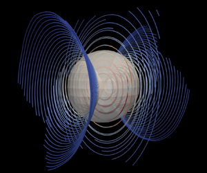
Let us consider an uncharged neutrally buoyant dielectric droplet suspended in a weakly conducting fluid medium as shown in figure 1. The volumes occupied by the droplet and surrounding fluid are denoted by  $V^-$ and $V^+$, respectively. In the absence of an electric field, the droplet remains spherical. However, under the influence of an applied field, the shape deviates from a sphere and undergoes small ellipsoidal deformations in the limit of high viscosity and high surface tension. The unit normal vector on the droplet–fluid interface ${S}$ is denoted by $\boldsymbol {n}$ and points into the suspending fluid medium. The electric field may point in any direction, and without loss of generality we choose a coordinate system in which it is aligned with the $y$-axis. Let $(\epsilon ^{\pm },\sigma ^{\pm },\mu ^{\pm })$ be the dielectric permittivities, electric conductivities and dynamic viscosities of the two fluids, respectively. Non-dimensionalization of the material properties yields three dimensionless groups, typically defined as
 \begin{equation} R=\frac{\sigma^+}{\sigma^-},\quad Q= \frac{\epsilon^-}{\epsilon^+},\quad \lambda =\frac{\mu^-}{\mu^+}. \end{equation}
The low-drop-viscosity limit  $\lambda \rightarrow 0$ describes a bubble, whereas $\lambda \rightarrow \infty$ describes a rigid particle. The product $RQ$ can also be interpreted as the ratio of the inner to outer charge relaxation times:
 \begin{equation} RQ=\frac{\tau^-}{\tau^+}\quad \mbox{where}\ \tau^\pm=\frac{\epsilon^\pm}{\sigma^\pm}. \end{equation}
Figure 1. Problem definition. (a) Prolate- and (b) oblate-shaped drops in the Taylor regime. Quadrupolar flow fields inside and outside the drop advect charges (depicted as  $+$ and $-$ symbols) from equator to poles in the prolate case and from poles to equator in the oblate case. Here $V^{\pm }$ denote the exterior and interior domains, respectively, and $(\epsilon ^\pm , \sigma ^\pm ,\mu ^\pm )$ are the corresponding dielectric permittivities, electric conductivities and dynamic viscosities. (c) Tilted drop in the Quincke regime with both quadrupolar and rotational flow fields present. Here $L$ and $B$ denote the longest and shortest dimensions of the drop, while $\phi ^*$ is the angle between the direction of maximum deformation and the $x$-axis. The electric field is applied along the $y$-axis.
Under the assumptions of the Melcher–Taylor leaky-dielectric model (Melcher & Taylor Reference Melcher and Taylor1969), all charges in the domain are concentrated on the drop–fluid interface, so that the electric potential in both fluid domains is governed by Laplace's equation:
 \begin{equation} \nabla^{2}\varphi^{\pm}(\boldsymbol{x})=0 \quad \mbox{for}\ \boldsymbol{x}\in V^{\pm}. \end{equation}
The electric potential and the tangential component of the local electric field are continuous across the interface:
 \begin{equation} [\kern-1pt[ \varphi (\boldsymbol{x})]\kern-1pt] =0 \quad \mbox{and} \quad [\kern-1pt[ \boldsymbol{E}_t(\boldsymbol{x})]\kern-1pt] =\boldsymbol{0} \quad \mbox{for}\ \boldsymbol{x}\in S, \end{equation}
where  $\boldsymbol {E}^{\pm }_{t}=({{\boldsymbol{\mathsf{I}}}}-\boldsymbol {nn})\boldsymbol {\cdot } \boldsymbol {E}^{\pm }$ and $\boldsymbol {E}^{\pm }=-\boldsymbol {\nabla } \varphi ^{\pm }$. We have introduced the notation $[\kern-1pt[ \,f(\boldsymbol {x})]\kern-1pt] \equiv f^+(\boldsymbol {x}) - f^-(\boldsymbol {x})$ for any field variable $f(\boldsymbol {x})$ defined on both sides of the interface. The normal component of the electric field $E_{n}^{\pm }=\boldsymbol {n}\boldsymbol {\cdot }\boldsymbol {E}^{\pm }$ undergoes a jump due to the mismatch in electrical properties between the two media (Landau, Lifshitz & Pitaevskiì Reference Landau, Lifshitz and Pitaevskiì1984), resulting in a surface charge distribution $q(\boldsymbol {x})$ related to the normal displacement field by Gauss's law:
 \begin{equation} q(\boldsymbol{x})=[\kern-1pt[ \epsilon {E}_n(\boldsymbol{x})]\kern-1pt] \quad \mbox{for}\ \boldsymbol{x}\in S. \end{equation}
The surface charge density  $q$ obeys a conservation law that prescribes a balance between temporal changes in charge, Ohmic currents from the bulk and charge advection by the fluid flow with velocity $\boldsymbol {v}(\boldsymbol {x})$ on the drop surface. Accordingly, it satisfies the conservation equation
 \begin{equation} \frac{\partial q}{\partial t} + [\kern-1pt[ \sigma {E}_n]\kern-1pt] +\boldsymbol{\nabla}_{s} \boldsymbol{\cdot} (q\boldsymbol{v})=0 \quad \mbox{for}\ \boldsymbol{x}\in S, \end{equation}
where  $\boldsymbol {\nabla }_{s}\equiv ({{\boldsymbol{\mathsf{I}}}}-\boldsymbol {nn})\boldsymbol {\cdot }\boldsymbol {\nabla }$ is the surface gradient operator. Since the droplet and medium are leaky dielectrics, freely moving charged ions in the bulk are assumed to be present in negligible quantities and only surface charges are assumed to exist in the physical domain. A detailed derivation of the leaky-dielectric model from a more generic electrodiffusion model is provided in the recent work of Mori & Young (Reference Mori and Young2018).
The fluid velocity field  $\boldsymbol {v}^{\pm }(\boldsymbol {x})$ and corresponding pressure field $p^{\pm }(\boldsymbol {x})$ satisfy the Stokes equations in both fluid domains:
 \begin{equation} -\mu^{\pm}\nabla^{2}\boldsymbol{v}^{\pm}+\boldsymbol{\nabla} p^{\pm}=\boldsymbol{0}\quad \mbox{and}\quad \boldsymbol{\nabla}\boldsymbol{\cdot}\boldsymbol{v}^{\pm}=0 \quad \mbox{for}\ \boldsymbol{x}\in V^{\pm}. \end{equation}
The fluid velocity is continuous across the interface  $S$,
$S$,
 \begin{equation} [\kern-1pt[ \boldsymbol{v}(\boldsymbol{x})]\kern-1pt] =\boldsymbol{0} \quad \mbox{for}\ \boldsymbol{x}\in S, \end{equation}
and the shape of the interface, parametrized by an implicit equation  $\xi (\boldsymbol {x},t)=0$, deforms as a material surface,
 \begin{equation} \frac{\mathrm{D}\xi}{\mathrm{D}t}=\frac{\partial \xi}{\partial t}+ \boldsymbol{v}\boldsymbol{\cdot}\boldsymbol{\nabla} \xi =0 \quad \mbox{for}\ \boldsymbol{x}\in S. \end{equation}
The dynamic boundary condition requires that the jumps in electric and hydrodynamic tractions across the interface balance surface tension forces:
 \begin{equation} [\kern-1pt[\,\boldsymbol{f}_{E}]\kern-1pt] + [\kern-1pt[\,\boldsymbol{f}_{H}]\kern-1pt] =\gamma (\boldsymbol{\nabla}_{s}\boldsymbol{\cdot}\boldsymbol{n})\boldsymbol{n} \quad \mbox{for}\ \boldsymbol{x}\in S.\end{equation}
Here,  $\gamma$ is the constant surface tension and $\boldsymbol {\nabla }_{s} \boldsymbol {\cdot }\boldsymbol {n}=2\kappa _{m}$ is twice the mean surface curvature. The jumps in tractions are obtained in terms of the Maxwell stress tensor ${{\boldsymbol{\mathsf{T}}}}_{E}$ and hydrodynamic stress tensor ${{\boldsymbol{\mathsf{T}}}}_{H}$ as
 \begin{gather} [\kern-1pt[\,\boldsymbol{f}_{E}]\kern-1pt] = \boldsymbol{n}\boldsymbol{\cdot}[\kern-1pt[{{\boldsymbol{\mathsf{T}}}}_{E}]\kern-1pt]= \boldsymbol{n}\boldsymbol{\cdot}[\kern-1pt[ \epsilon (\boldsymbol{EE}-\tfrac{1}{2}E^{2}{{\boldsymbol{\mathsf{I}}}})]\kern-1pt], \end{gather}
 \begin{gather}[\kern-1pt[\,\boldsymbol{f}_{H}]\kern-1pt] =\boldsymbol{n}\boldsymbol{\cdot}[\kern-1pt[{{\boldsymbol{\mathsf{T}}}}_{H}]\kern-1pt] = \boldsymbol{n}\boldsymbol{\cdot} [\kern-1pt[-p{{\boldsymbol{\mathsf{I}}}}+\mu (\boldsymbol{\nabla} \boldsymbol{v}+\boldsymbol{\nabla}\boldsymbol{v}^{\textrm{T}} )]\kern-1pt]. \end{gather}
The jump in electric tractions can also be expressed as
 \begin{equation} [\kern-1pt[\,\boldsymbol{f}_{E}]\kern-1pt] =[\kern-1pt[ \epsilon E_{n} ]\kern-1pt] \boldsymbol{E}_{t}+\tfrac{1}{2}[\kern-1pt[ \epsilon(E_{n}^{2}-E_{t}^{2})]\kern-1pt] \boldsymbol{n} =q\boldsymbol{E}_{t}+ [\kern-1pt[ p_{E}]\kern-1pt] \boldsymbol{n}.\end{equation}
The first term on the right-hand side captures the tangential electric force acting on the interfacial charge, while the second term captures normal electric stresses and can be interpreted as a jump in electric pressure  $p_E=\frac {1}{2}\epsilon (E_n^2-E_t^2)$ (Lac & Homsy Reference Lac and Homsy2007).
The characteristic length and time scales of the problem are the initial radius of the droplet  $a_d$ and the Maxwell–Wagner relaxation time $\tau _{MW}$, which is the time scale for polarization of the drop surface upon application of the field (Das & Saintillan Reference Das and Saintillan2013):
 \begin{equation} \tau_{MW}=\frac{\epsilon^- +2\epsilon^+}{\sigma^- +2\sigma^+}. \end{equation}
Non-dimensionalization of the electric tractions with  $\epsilon ^+ E_0^2$, hydrodynamic tractions with $\mu ^+ a/\tau _{MW}$ and surface tension forces with $\gamma /a$ gives rise to two additional dimensionless numbers. They consist of the electric capillary number $Ca_E$, denoting the ratio of electric to capillary forces, and the electric Mason number $Ma$, denoting the ratio of viscous to electric stresses:
 \begin{equation} Ca_{E}=\frac{a_d\epsilon^+ E_{0}^{2}}{\gamma},\quad Ma = \frac{\mu^+}{\epsilon^+ \tau_{MW}E_{0}^2}. \end{equation}
The Mason number is inversely proportional to the electric Reynolds number  $Re_E$ sometimes used in the literature (Salipante & Vlahovska Reference Salipante and Vlahovska2010; Lanauze et al. Reference Lanauze, Walker and Khair2015; Yariv & Frankel Reference Yariv and Frankel2016) and defined as
 \begin{equation} Re_E=\frac{1}{Ma}\frac{1+2R}{R(Q+2)}. \end{equation}
 Since we choose  $\tau _{MW}$ as the time scale for the problem, the Mason number, $Ma$, appears in the stress balance equation (3.26). Alternatively, one can choose the EHD straining flow time, $\tau _{HD} = \mu ^+(1+\lambda )/(\epsilon ^+ E_0^2)$, as the relevant time scale for the problem, which would result in the Mason number, $Ma$, appearing in the charge conservation equation (3.36), as done in some previous studies (He et al. Reference He, Salipante and Vlahovska2013).
3. Problem solution
We now present the solution to the governing equations introduced above using a small-deformation or domain perturbation theory (Taylor & Acrivos Reference Taylor and Acrivos1964; Matunobu Reference Matunobu1966; Barthès-Biesel & Acrivos Reference Barthès-Biesel and Acrivos1973; Rallison Reference Rallison1980). Note that the solutions are expressed in the laboratory frame of reference.
3.1. Shape of a slightly deformed drop
Let us parametrize the drop–fluid interface as  $\xi \equiv r - [1+ \delta f(\theta ,\phi ,t)]=0$, where $(r,\theta ,\phi )$ are spherical coordinates with polar angle $\theta$ and azimuthal angle $\phi$. Departures from the spherical shape are assumed to be small, as evidenced by the small-deformation parameter $\delta$ to be defined more precisely later (see § 3.5). The shape $f$ of the drop is expanded on the basis of spherical harmonics:
 \begin{equation} f(\theta,\phi,t) = \sum_{l=0}^{\infty} \sum_{m=-l}^{l} \mathcal{L}_{ml}(\cos \theta) [\,f_{ml}(t) \cos m\phi + \tilde{f}_{ml}(t)\sin m\phi], \end{equation}
where  $\mathcal {L}_{ml}(\cos \theta )$ are the associated Legendre functions of order $m$ and degree $l$. Owing to the quadratic nature of electric stresses, the applied field induces perturbations in the drop's shape that are of even order (Das & Saintillan Reference Das and Saintillan2017b). Retaining terms to the leading order of deformation ( $l=2$), we obtain the following expression for the shape:
 \begin{align} f(\theta,\phi,t)&= \tfrac{1}{2}(3\cos^2\theta - 1)\,f_{02}(t) - 3\cos\theta\sin\theta \, [\,f_{12}(t) \cos\phi + \tilde{f}_{12}(t) \sin\phi] \nonumber\\ &\quad +3\sin^2\theta \, [\,f_{22}(t)\cos 2\phi + \,\tilde{f}_{22}(t) \sin2\phi]. \end{align}
The time-dependent coefficients  $\,f_{ml}$ and $\tilde {f}_{ml}$ are unknown and to be determined as part of the solution. Using (3.2), we can obtain the unit normal vector and mean curvature as
 \begin{equation} \boldsymbol{n} = \left[\frac{\boldsymbol{\nabla} \xi}{|\boldsymbol{\nabla} \xi|}\right]_{r=1}=\boldsymbol{\hat{r}} - \delta \boldsymbol{\nabla} f + {O}(\delta^2),\quad \kappa_m = \tfrac{1}{2} \boldsymbol{\nabla}_s \boldsymbol{\cdot} \boldsymbol{n}. \end{equation}
Detailed expressions for  $\boldsymbol {n}$ and $\kappa _m$ are provided in appendix A.
3.2. Electric problem
The solution for the electric potential in a spherical geometry is best written in terms of harmonic multipoles (Jackson Reference Jackson1998), with the leading-order term corresponding to a dipole in this problem. Higher-order multipoles can arise even at first order in deformation due to the nonlinear charge conservation equation, but we neglect them here. The leading order of these higher-order multipoles is  ${O}(Ma^{-n} \lambda ^{-n})$ with $n>2$ and they become stronger with decreasing Mason number and viscosity ratio (see §§ 3.6 and 5.2 for details). Our theory is therefore valid for drop–fluid systems in which the straining component of the flow is relatively weak. It is also noted that including higher-order electric multipoles will in turn induce higher-order shape multipoles in (3.2).
The induced dipole moment on the drop is denoted by  $\boldsymbol {P} = (P_x,P_y,P_z)$ and is non-dimensionalized by $a^3E_0$. The electric potential, non-dimensionalized by $aE_0$, at location $\boldsymbol {r}=r(\sin \theta \cos \phi ,\sin \theta \sin \phi ,\cos \phi )$ outside and inside the drop is then given by
 \begin{equation} \varphi^+ = -\boldsymbol{\hat{e}}\boldsymbol{\cdot} \boldsymbol{r} + \frac{\boldsymbol{P}\boldsymbol{\cdot}\boldsymbol{r}}{r^3}, \quad \varphi^- = -\boldsymbol{\hat{e}}\boldsymbol{\cdot} \boldsymbol{r} + \boldsymbol{P}\boldsymbol{\cdot}\boldsymbol{r}, \end{equation}
respectively, where  $\boldsymbol {\hat {e}}=\boldsymbol {E}_0/E_0$ denotes the direction of the external field. Equations (3.4a,b) satisfy the boundary conditions (2.4a,b). The normal component of the electric field is discontinuous, while its tangential components are continuous. Note that, in the leading-order perturbation analysis, the boundary conditions are enforced on the surface of the undeformed sphere $r=a$. Therefore, the leading-order electric field components are
 \begin{gather} E^+_r = P^+_x\sin\theta\cos\phi + P^+_y \sin\theta\sin\phi + P^+_z \cos \theta, \end{gather}
 \begin{gather}E^-_r = P^-_x \sin\theta\cos\phi + P^-_y \sin\theta\sin\phi + P_z^- \cos \theta, \end{gather}
 \begin{gather}E_\theta = P^-_x\cos\theta \cos\phi + P^-_y\cos\theta\sin\phi - P^-_z\sin \theta, \end{gather}
 \begin{gather}E_\phi = - P^-_x \sin\phi + P^-_y\cos\phi. \end{gather}
We have introduced the short-hand notation  $\boldsymbol {P}^+=\boldsymbol {\hat {e}}+2\boldsymbol {P}$ and $\boldsymbol {P}^-=\boldsymbol {\hat {e}}-\boldsymbol {P}$ for the coefficients appearing in the combined electric field accounting for the applied field and induced dipole moment. Doing so allows us to keep the direction $\boldsymbol {\hat {e}}$ of the applied field arbitrary, only to be specified when dealing with the charge conservation equation in § 3.6. For example, if the electric field is applied in the $y$-direction, we substitute $P^+_y = 1 + 2P_y$, $P^-_y = 1 - P_y$, $P^+_{x,z} = 2P_{x,z}$ and $P^-_{x,z} = -P_{x,z}$.
The surface charge density, given by Gauss's law, and the jump in Ohmic current at the interface can both also be expressed in terms of surface harmonics as
 \begin{gather} q = E^+_r - Q E^-_r = q_{01} \cos \theta+ q_{11} \sin\theta\cos\phi + \tilde{q}_{11} \sin\theta\sin\phi, \end{gather}
 \begin{gather}\boldsymbol{n} \boldsymbol{\cdot} [\kern-1pt[\,\boldsymbol{j} ]\kern-1pt] = RE^+_r - E^-_r = j_{n,01} \cos \theta + j_{n,11} \sin\theta\cos\phi + \tilde{j}_{n,11} \sin\theta\sin\phi, \end{gather}
where the coefficients  $q_{ml}$ and $j_{n,ml}$ are linear functions of the dipole moment:
 \begin{gather} q_{01} = P_z^+ - Q P_z^-, \quad q_{11} = P_x^+ - Q P_x^-, \quad \tilde{q}_{11} = P_y^+ - Q P_y^-, \end{gather}
 \begin{gather}j_{n,01} = P_z^+ - Q P_z^-, \quad j_{n,11} = P_x^+ - Q P_x^-, \quad \tilde{j}_{n,11} = P_y^+ - Q P_y^-. \end{gather}
The radial, polar and azimuthal components of the jump in electric tractions in (2.13) can similarly be written as
 \begin{align} [\kern-1pt[ p_E ]\kern-1pt] &= [\kern-1pt[ p_E ]\kern-1pt]_{00} + [\kern-1pt[ p_E ]\kern-1pt]_{02} \cos^2\theta + ([\kern-1pt[ p_E ]\kern-1pt]_{12} \cos \phi + [\kern-1pt[ \widetilde{p_E} ]\kern-1pt]_{12} \sin \phi ) \sin 2\theta \nonumber\\ &\quad + ([\kern-1pt[ p_E ]\kern-1pt]_{22} \cos 2\phi + [\kern-1pt[ \widetilde{p_E} ]\kern-1pt]_{22} \sin2\phi ) \sin^2\theta, \end{align}
 \begin{align} qE_\theta &= qE_{\theta ,02} \sin 2\theta+qE_{\theta ,10} \cos \phi + \widetilde{q E}_{\theta ,10} \sin \phi \nonumber\\ &\quad + (qE_{\theta ,12} \cos\phi + \widetilde{q E}_{\theta ,12} \sin \phi) \cos 2\theta + (qE_{\theta ,22} \cos 2\phi + \widetilde{q E}_{\theta ,22} \sin 2\phi) \sin 2\theta \end{align}
and
 \begin{align} qE_\phi &= qE_{\phi ,01} \sin \theta + (qE_{\phi ,11} \cos\phi + \widetilde{q E}_{\phi ,11} \sin \phi ) \cos \theta \nonumber\\ &\quad + (qE_{\phi ,21} \cos 2\phi + \widetilde{q E}_{\phi ,21} \sin 2\phi) \sin \theta. \end{align}
The unknown coefficients in this case are quadratic functions of the dipole moments and are provided in appendix C. It is instructive to notice that the radial, polar and azimuthal components of the tractions contain harmonic functions of degrees two, two and one, and one, respectively. We also note that the terms containing  $qE_{\theta ,10}$, $\widetilde {q E}_{\theta ,10}$ and $qE_{\phi ,01}$ in the tangential tractions capture the net electric torque acting on the droplet.
3.3. Flow problem
We solve the Stokes equations (2.7a,b) in spherical coordinates using Lamb's general solution (Happel & Brenner Reference Happel and Brenner1965; Kim & Karrila Reference Kim and Karrila2013). The pressure  $p$ satisfies Laplace's equation and constitutes the particular solution for the Stokes momentum equation, while the homogeneous solution consists of the velocity potential $\varPhi$ and toroidal flow field $\chi$. Inside the drop, only growing harmonics are retained,
 \begin{gather} p_l = r^l \sum_{m=0}^l \mathcal{L}_{ml} (\cos\theta)[a_{ml}\cos m\phi + \tilde{a}_{ml}\sin m\phi], \end{gather}
 \begin{gather}\varPhi_l = r^l \sum_{m=0}^l \mathcal{L}_{ml} (\cos\theta)[b_{ml}\cos m\phi + \tilde{b}_{ml}\sin m\phi], \end{gather}
 \begin{gather}\chi_l = r^l \sum_{m=0}^l \mathcal{L}_{ml} (\cos\theta)[c_{ml}\cos m\phi + \tilde{c}_{ml}\sin m\phi], \end{gather}
while decaying harmonics are used outside,
 \begin{gather} p_{-l-1} = r^{-l-1} \sum_{m=0}^l \mathcal{L}_{ml} (\cos\theta)[A_{ml}\cos m\phi + \tilde{A}_{ml}\sin m\phi], \end{gather}
 \begin{gather}\varPhi_{-l-1} = r^{-l-1} \sum_{m=0}^l \mathcal{L}_{ml} (\cos\theta)[B_{ml}\cos m\phi + \tilde{B}_{ml}\sin m\phi], \end{gather}
 \begin{gather}\chi_{-l-1} = r^{-l-1} \sum_{m=0}^l \mathcal{L}_{ml} (\cos\theta)[C_{ml}\cos m\phi + \tilde{C}_{ml}\sin m\phi]. \end{gather}
The velocity fields inside and outside the drop are written as
 \begin{equation} \begin{aligned} \boldsymbol{v}^- & = \sum_{l=1}^\infty \left[\frac{(l+3)r^2\boldsymbol{\nabla}p_l - 2lp_l\boldsymbol{r}}{2\lambda(l+1)(2l+3)} + \boldsymbol{\nabla}\varPhi_l + \boldsymbol{\nabla}\chi_l \times \boldsymbol{r} \right], \\ \boldsymbol{v}^+ & = \sum_{l=1}^\infty \left[\frac{-(l-2)r^2\boldsymbol{\nabla}p_{-l-1} + 2(l+1)p_{-l-1}\boldsymbol{r}}{2 l(2l-1)} \right] + \sum_{l=0}^\infty \left[\boldsymbol{\nabla}\varPhi_{-l-1} + \boldsymbol{\nabla}\chi_{-l-1} \times \boldsymbol{r} \right]. \end{aligned} \end{equation}
and the corresponding pressure fields are  $p^- = \sum _{l=0}^{\infty } p_l$ and $p^+ = \sum _{l=-1}^{\infty } p_{-l-1}$. The velocity and pressure fields are then used to obtain the hydrodynamic tractions inside and outside,
 \begin{equation} \boldsymbol{f}_H^\pm = -\boldsymbol{\hat{r}}p^\pm + \mu^\pm \boldsymbol{\hat{r}} \boldsymbol{\cdot} (\boldsymbol{\nabla} \boldsymbol{v}^\pm + \boldsymbol{\nabla} \boldsymbol{v}^{\pm \textrm{T}}) + {O}(\delta), \end{equation}
which must balance electric stresses as well as capillary forces. Inspecting the radial and tangential components of these various tractions, we can deduce the harmonics that need to be retained:
 \begin{gather} \boldsymbol{f}_H^- =-\boldsymbol{\hat{r}} p_0^- + \tfrac{8}{21} r\boldsymbol{\nabla} p_2 - \tfrac{19}{21} \boldsymbol{\hat{r}} p_2 + 2\lambda r^{-1} \boldsymbol{\nabla}\varPhi_2, \end{gather}
 \begin{gather}\boldsymbol{f}_H^+ =-\boldsymbol{\hat{r}} p_0^+ + \tfrac{1}{2} r \boldsymbol{\nabla} p_{-3} - \tfrac{3}{2} \boldsymbol{\hat{r}}p_{-3} - 8 r^{-1} \boldsymbol{\nabla}\varPhi_{-3} - 3 \boldsymbol{\nabla}\chi_{-2} \times \boldsymbol{\hat{r}}. \end{gather}
 Using the identity  $\boldsymbol {r} \boldsymbol {\cdot } \boldsymbol {\nabla } p_l = lp_l$, we find the radial, polar and azimuthal components of the jump in hydrodynamic tractions to be
 \begin{gather} \boldsymbol{\hat{r}} \boldsymbol{\cdot} [\kern-1pt[\,\boldsymbol{f}_H ]\kern-1pt] = - [\kern-1pt[ p_0 ]\kern-1pt] - 3 p_{-3} + 24 \varPhi_{-3} + \tfrac{1}{7} p_2 - 4\lambda \varPhi_2, \end{gather}
 \begin{gather}\boldsymbol{\hat{\theta}} \boldsymbol{\cdot} [\kern-1pt[\,\boldsymbol{f}_H ]\kern-1pt] = \tfrac{1}{2} \boldsymbol{\hat{\theta}} \boldsymbol{\cdot} \boldsymbol{\nabla} p_{-3} - (8\boldsymbol{\hat{\theta}} \boldsymbol{\cdot} \boldsymbol{\nabla}\varPhi_{-3} + 3 \boldsymbol{\hat{\phi}} \boldsymbol{\cdot} \boldsymbol{\nabla}\chi_{-2}) - \tfrac{8}{21} \boldsymbol{\hat{\theta}} \boldsymbol{\cdot} \boldsymbol{\nabla} p_2 - 2 \lambda \boldsymbol{\hat{\theta}} \boldsymbol{\cdot} \boldsymbol{\nabla}\varPhi_2, \end{gather}
 \begin{gather}\boldsymbol{\hat{\phi}} \boldsymbol{\cdot} [\kern-1pt[\,\boldsymbol{f}_H ]\kern-1pt] = \tfrac{1}{2} \boldsymbol{\hat{\phi}} \boldsymbol{\cdot} \boldsymbol{\nabla} p_{-3} - (8 \boldsymbol{\hat{\phi}} \boldsymbol{\cdot} \boldsymbol{\nabla}\varPhi_{-3} - 3 \boldsymbol{\hat{\theta}} \boldsymbol{\cdot} \boldsymbol{\nabla}\chi_{-2}) - \tfrac{8}{21} \boldsymbol{\hat{\phi}} \boldsymbol{\cdot} \boldsymbol{\nabla} p_2 - 2 \lambda \boldsymbol{\hat{\phi}} \boldsymbol{\cdot} \boldsymbol{\nabla}\varPhi_2. \end{gather}
The radial stresses are conveniently expressed in terms of spherical harmonics of second degree  $D$, while for the tangential stresses it is convenient to assume $({{\boldsymbol{\mathsf{I}}}}-\boldsymbol {rr}) \boldsymbol {\cdot } [\kern-1pt[ \,\boldsymbol {f}_H ]\kern-1pt] =({{\boldsymbol{\mathsf{I}}}}-\boldsymbol {rr}) \boldsymbol {\cdot } (\boldsymbol {\nabla } G + \boldsymbol {\nabla } F \times \boldsymbol {\hat {r}})$, where $G$ and $F$ are spherical harmonics of second and first degree, respectively. The hydrodynamic stresses are then compactly written as
 \begin{align} \boldsymbol{\hat{r}} \boldsymbol{\cdot} [\kern-1pt[\,\boldsymbol{f}_H ]\kern-1pt] &= -[\kern-1pt[ p_0 ]\kern-1pt] + [\tfrac{1}{2}(3\cos^2\theta - 1)D_{02} - 3\cos\theta\sin\theta\, (D_{12} \cos\phi + \tilde{D}_{12} \sin\phi) \nonumber\\ &\quad +3\sin^2\theta\,(D_{22} (\cos 2\phi) + \tilde{D}_{22} \sin(2\phi))], \end{align}
 \begin{align} \boldsymbol{\hat{\theta}} \boldsymbol{\cdot} [\kern-1pt[\,\boldsymbol{f}_H ]\kern-1pt] &= 3\sin 2\theta\,(-0.5G_{02} + G_{22} \cos 2\phi + \tilde{G}_{22} \sin 2\phi) \nonumber\\ &\quad -3\cos 2\theta \,(G_{12} \cos\phi + \tilde{G}_{12} \sin\phi) + F_{11}\sin\phi - \tilde{F}_{11} \cos\phi \end{align}
and
 \begin{align} \boldsymbol{\hat{\phi}} \boldsymbol{\cdot} [\kern-1pt[\,\boldsymbol{f}_H ]\kern-1pt] &= 3\cos \theta \, (G_{12} \sin \phi - \tilde{G}_{12} \cos \phi) - 6\sin \theta \,(G_{22} \sin 2\phi - \tilde{G}_{22} \cos 2\phi) ] \nonumber\\ &\quad + F_{01}\sin\theta + \cos\theta \, (F_{11} \cos\phi + \tilde{F}_{11}\sin\phi), \end{align}
where the stress coefficients are given by linear combinations of the flow coefficients:
 \begin{gather} D_{ml} = -3 A_{ml} + 24B_{ml} + \tfrac{1}{7}a_{ml} - 4 \lambda b_{ml}, \end{gather}
 \begin{gather}G_{ml} = \tfrac{1}{2} A_{ml} - 8B_{ml} - \tfrac{8}{21} a_{ml} - 2 \lambda b_{ml}, \end{gather}
 \begin{gather}F_{ml} = -3 C_{ml}. \end{gather}
At this order of approximation, (3.13) for the velocity fields becomes
 \begin{equation} \boldsymbol{v}^- = \boldsymbol{\nabla}\chi_1 \times \boldsymbol{r} + \frac{5 r^2 \boldsymbol{\nabla} p_2 - 4p_2 \boldsymbol{r}}{42\lambda} + \boldsymbol{\nabla}\varPhi_2,\quad \boldsymbol{v}^+ = \boldsymbol{\nabla}\chi_{-2} \times \boldsymbol{r} + \tfrac{1}{2}p_{-3} \boldsymbol{r} + \boldsymbol{\nabla}\varPhi_{-3} . \end{equation}
3.4. Kinematic boundary condition
The no-slip and no-penetration boundary conditions of (2.8) and (2.9) are
 \begin{equation} v_\theta^+ = v_\theta^-, \quad v_\phi^+ = v_\phi^-,\quad v_r^+ - \delta \boldsymbol{v}^+ \boldsymbol{\cdot} \boldsymbol{\nabla} f = v_r^- - \delta \boldsymbol{v}^- \boldsymbol{\cdot} \boldsymbol{\nabla} f= \delta \dot{f}, \end{equation}
which provide relationships between the flow coefficients inside and outside the droplet. First, continuity of the polar and azimuthal components of the velocity yields the two relations
 \begin{equation} \frac{5}{42 \lambda}a_{ml} + b_{ml} = B_{ml} \quad \mathrm{and} \quad c_{ml}=C_{ml}. \end{equation}
The no-penetration boundary condition (3.20c) has two terms that are of  ${O}(\delta )$, which implies that $v_r^\pm$ must be of order ${O}(\delta )$ as well. Since $v_r^\pm \sim \lambda ^{-1}$, we require $\lambda ^{-1} = {O}(\delta )$, making the theory most accurate for viscous droplets that undergo small deformations due to high capillary forces. The radial components of the velocity inside and outside the drop are
 \begin{equation} v_r^- = \frac{1}{7 \lambda} r p_2 + \frac{2}{r} \varPhi_2 \quad \mathrm{and} \quad v_r^+ = \frac{1}{2} rp_{-3} - \frac{3}{r}\varPhi_{-3}. \end{equation}
The no-penetration boundary condition in the radial direction gives us relations involving the temporal derivatives of the shape and the flow coefficients,
 \begin{equation} \frac{1}{7\lambda}a_{ml} + 2b_{ml} = \frac{1}{2} A_{ml} - 3B_{ml} = \delta (\dot{f}_{ml} + [\boldsymbol{v} \boldsymbol{\cdot} \boldsymbol{\nabla} f]_{ml} ), \end{equation}
where we have introduced the following notation for the nonlinear product  $\boldsymbol {v} \boldsymbol {\cdot } \boldsymbol {\nabla } f$:
 \begin{align} [\boldsymbol{v} \boldsymbol{\cdot} \boldsymbol{\nabla} f] &= \tfrac{1}{2}(3\cos^2\theta - 1)[\boldsymbol{v} \boldsymbol{\cdot} \boldsymbol{\nabla} f]_{02} - 3\cos\theta\sin\theta\,([\boldsymbol{v} \boldsymbol{\cdot} \boldsymbol{\nabla} f]_{12} \cos\phi \nonumber\\ &\quad + \widetilde{[\boldsymbol{v} \boldsymbol{\cdot} \boldsymbol{\nabla} f]}_{12} \sin\phi) + 3\sin^2\theta \,([\boldsymbol{v} \boldsymbol{\cdot} \boldsymbol{\nabla} f]_{22} \cos 2\phi + \widetilde{[\boldsymbol{v} \boldsymbol{\cdot} \boldsymbol{\nabla} f]}_{22} \sin2\phi). \end{align}
The coefficients  $[\boldsymbol {v} \boldsymbol {\cdot } \boldsymbol {\nabla } f]_{ml}$ are quadratic functions of $C_{ml}$ and $\,f_{ml}$ and are provided in appendix C. Note that $\boldsymbol {v} \boldsymbol {\cdot } \boldsymbol {\nabla } f$ only involves rigid-body rotation, as it is independent of viscosity, so that the leading-order term in (3.20c) is ${O}(\delta )$. Physically, it simply represents rotation of the droplet shape with the angular velocity $C$. We choose to express all the flow coefficients in terms of coefficients $B$ and $C$ (through $[\boldsymbol {v} \boldsymbol {\cdot } \boldsymbol {\nabla } f]$) as well as the shape transient $\dot {f}$:
 \begin{gather} A_{ml} = 2 \{\delta (\,\dot{f}_{ml} + [\boldsymbol{v} \boldsymbol{\cdot} \boldsymbol{\nabla} f]_{ml} ) + 3B_{ml} \}, \end{gather}
 \begin{gather}a_{ml} = \tfrac{21}{2} \lambda \{ -\delta (\,\dot{f}_{ml} + [\boldsymbol{v} \boldsymbol{\cdot} \boldsymbol{\nabla} f]_{ml} ) + 2B_{ml} \}, \end{gather}
 \begin{gather}b_{ml} = \tfrac{1}{4} \{5\delta (\,\dot{f}_{ml} + [\boldsymbol{v} \boldsymbol{\cdot} \boldsymbol{\nabla} f]_{ml} ) - 6B_{ml} \}. \end{gather}
Flows associated with coefficients  $B$ and $C$ represent straining and rigid-body rotational flows, respectively.
3.5. Dynamic boundary condition
The dimensionless stress balance on the drop interface reads
 \begin{equation} [\kern-1pt[ p_E ]\kern-1pt] \boldsymbol{n} + q (E_\theta \boldsymbol{\hat{\theta}} + E_\phi \boldsymbol{\hat{\phi}} )+ Ma [\kern-1pt[\,\boldsymbol{f}_H ]\kern-1pt] = \frac{2}{Ca_E} \kappa_m \boldsymbol{n}. \end{equation}
We retain terms up to order  ${O}(\delta )$ in this equation. In the radial direction, this reads
 \begin{equation} [\kern-1pt[ p_E ]\kern-1pt]+ Ma\, \boldsymbol{\hat{r}} \boldsymbol{\cdot} [\kern-1pt[\,\boldsymbol{f}_H ]\kern-1pt] = \frac{2}{Ca_E}(1+2\delta f). \end{equation}
Using orthogonality of spherical harmonics, we obtain one set of relations between the dipole moments, flow and shape coefficients:
 \begin{equation} \begin{aligned} & [\kern-1pt[ p_E ]\kern-1pt]_{00} - Ma ([\kern-1pt[ p_0 ]\kern-1pt]+ \tfrac{1}{2} D_{02} ) = 2Ca_E^{-1} (1 - \delta \,f_{02}),\quad [\kern-1pt[ p_E ]\kern-1pt]_{02} + \tfrac{3}{2} Ma D_{02} = 6 Ca_E^{-1} \delta \,f_{02}, \\ & [\kern-1pt[ p_E ]\kern-1pt]_{12} - \tfrac{3}{2} Ma D_{12} = -6 Ca_E^{-1} \delta \,f_{12},\quad [\kern-1pt[ \widetilde{p_E} ]\kern-1pt]_{12} - \tfrac{3}{2} Ma \tilde{D}_{12} = -6 Ca_E^{-1} \delta \tilde{f}_{12}, \\ & [\kern-1pt[ p_E ]\kern-1pt]_{22} + 3 Ma D_{22} = 12 Ca_E^{-1} \delta \,f_{22}, \quad [\kern-1pt[ \widetilde{p_E} ]\kern-1pt]_{22} + 3 Ma \tilde{D}_{22} = 12 Ca_E^{-1} \delta \tilde{f}_{22}, \end{aligned} \end{equation}
where the hydrodynamic radial stress coefficients  $D$ are expressed in terms of the flow and shape coefficients using (3.18) and (3.25) as
 \begin{equation} D_{ml} = 3(2 + 3\lambda) B_{ml} - \tfrac{1}{2}\delta (12 + 13\lambda) (\,\dot{f}_{ml} + [\boldsymbol{v} \boldsymbol{\cdot} \boldsymbol{\nabla} f]_{ml} ). \end{equation}
The  ${O}(1)$ term on the right-hand side of the first equation in (3.28) is balanced by $[\kern-1pt[ p_0]\kern-1pt]$ and captures the Young–Laplace pressure jump due to surface tension in the undeformed state.
A second set of relations is obtained from the polar stress boundary condition
 \begin{equation} q E_\theta + Ma\, \boldsymbol{\hat{\theta}} \boldsymbol{\cdot} [\kern-1pt[\,\boldsymbol{f}_H ]\kern-1pt] = 0, \end{equation}
which, after applying orthogonality, yields
 \begin{equation} \begin{aligned} & \tilde{F}_{11} = \frac{1}{Ma} qE_{\theta ,10} , \quad F_{11} = - \frac{1}{Ma} \widetilde{q E}_{\theta ,10}, \\ & G_{02} = \frac{2}{3Ma} qE_{\theta ,02}, \quad G_{12} = \frac{1}{3Ma} qE_{\theta ,12} , \quad \tilde{G}_{12} = \frac{1}{3Ma} \widetilde{q E}_{\theta ,12}, \\ & G_{22} = - \frac{1}{3Ma} qE_{\theta ,22} , \quad \tilde{G}_{22} = - \frac{1}{3Ma} \widetilde{q E}_{\theta, 22} , \end{aligned} \end{equation}
where  $G$ and $F$, similar to $D$, are expressed in terms of the flow and shape coefficients as
 \begin{equation} F_{ml} = -3C_{ml}, \quad G_{ml} = -5(1+\lambda)B_{ml} + \tfrac{1}{2}\delta (2+3\lambda) (\,\dot{f}_{ml} + [\boldsymbol{v} \boldsymbol{\cdot} \boldsymbol{\nabla} f]_{ml} ). \end{equation}
Balancing stress in the azimuthal direction,
 \begin{equation} q E_\phi + Ma\, \boldsymbol{\hat{\phi}} \boldsymbol{\cdot} [\kern-1pt[\,\boldsymbol{f}_H ]\kern-1pt] = 0, \end{equation}
gives us the same set of relations as in (3.31), with one additional relation,
 \begin{equation} F_{01} = \frac{1}{Ma} qE_{\phi ,01}. \end{equation}
 The driving force for the fluid velocity are the tangential electric stresses, which induce hydrodynamic tractions that scale as  ${O}(Ma^{-1})$. The magnitude of the resulting flow therefore is such that both electric and hydrodynamic radial tractions in (3.28) are of order ${O}(1)$. Balancing these tractions with surface tension forces requires us to choose $\delta \propto Ca^{-1}$. We choose to define the small-deformation parameter $\delta$ as
 \begin{equation} \delta=\frac{3Ca_E}{4(1+2R)^2}, \end{equation}
to be consistent with previous small-deformation theories (Taylor Reference Taylor1966). Physical quantities required to parametrize the drop shape, such as the extent of ellipsoidal deformations or tilt angle, are independent of this choice of  $\delta$. For given values of the dipole moments $P_{x,y,z}$, the relations provided in this section, (3.28), (3.31) and (3.34), completely solve the EHD flow problem.
3.6. Charge conservation equation
We now proceed to derive a dipole moment evolution equation in each direction starting from the charge conservation equation. In dimensionless form, it reads
 \begin{equation} \frac{\partial q}{\partial t}+\left(\frac{Q+2}{1+2R}\right)\boldsymbol{n}\boldsymbol{\cdot} [\kern-1pt[\,\boldsymbol{j}]\kern-1pt] +\boldsymbol{\nabla}_{s}\boldsymbol{\cdot} (q\boldsymbol{v})=0, \end{equation}
where the surface charge density and jump in electric current have been scaled by  $\epsilon E_0$ and $\sigma ^- E_0$, respectively. Taking moments of the charge conservation equation yields evolution equations for the charge coefficients:
 \begin{gather} \dot{q}_{01} + \left(\frac{Q+2}{1+2R}\right) j_{n,01} + \frac{3}{4{\rm \pi}} \int_{0}^{\rm \pi} \int_0^{2{\rm \pi}} [\boldsymbol{\nabla}_{s}\boldsymbol{\cdot} (q\boldsymbol{v})] [\cos \theta] \sin\theta \,\mathrm{d}\phi \,\mathrm{d}\theta = 0, \end{gather}
 \begin{gather}\dot{q}_{11} + \left(\frac{Q+2}{1+2R}\right) j_{n,11} + \frac{3}{4{\rm \pi}} \int_{0}^{\rm \pi} \int_0^{2{\rm \pi}} [\boldsymbol{\nabla}_{s}\boldsymbol{\cdot} (q\boldsymbol{v})] [\sin\theta\cos\phi] \sin\theta \,\mathrm{d}\phi \,\mathrm{d}\theta = 0, \end{gather}
 \begin{gather}\dot{\tilde{q}}_{11} + \left(\frac{Q+2}{1+2R}\right) \tilde{j}_{n,11} + \frac{3}{4{\rm \pi}} \int_{0}^{\rm \pi} \int_0^{2{\rm \pi}} [\boldsymbol{\nabla}_{s}\boldsymbol{\cdot} (q\boldsymbol{v})] [\sin\theta\sin\phi] \sin\theta \,\mathrm{d}\phi \,\mathrm{d}\theta = 0. \end{gather}
In view of (3.8a–c) and (3.9a–c), these can also be regarded as the governing equations for the components of the dipole moment  $\boldsymbol {P}$. The interfacial velocity is simply found from (3.19a,b) as $\boldsymbol {v}_s = \boldsymbol {v}^-|_{r=1} = \boldsymbol {v}^+|_{r=1}$. After substituting the expression for $\boldsymbol {v}_s$ along with kinematic boundary conditions and applying orthogonality of spherical harmonics, we obtain the final set of governing equations:
 \begin{align} & \dot{q}_{01} + \left(\frac{Q+2}{1+2R}\right) j_{n,01}+ \delta \Big\{\frac{4}{5}\left(\,\dot{f}_{02} + [\boldsymbol{v} \boldsymbol{\cdot} \boldsymbol{\nabla} f]_{02}\right) q_{01} \nonumber\\ &\quad -\frac{6}{5}\Big[\Big( \dot{\tilde{f}}_{12} + \widetilde{[\boldsymbol{v} \boldsymbol{\cdot} \boldsymbol{\nabla} f]}_{12}\Big) q_{11} + \left(\,\dot{f}_{12} + [\boldsymbol{v} \boldsymbol{\cdot} \boldsymbol{\nabla} f]_{12}\right)\tilde{q}_{11}\Big]\Big\} \nonumber\\ &\quad +\tilde{q}_{11}C_{11} - q_{11}\tilde{C}_{11} - \frac{6}{5} q_{01}B_{02} + \frac{9}{5}\Big(q_{11} B_{12} + \tilde{q}_{11}\tilde{B}_{12}\Big) = 0, \end{align}
 \begin{align} & \dot{q}_{11} + \left(\frac{Q+2}{1+2R}\right) j_{n,11} + \delta \Big\{-\frac{2}{5}\left(\,\dot{f}_{02} + [\boldsymbol{v} \boldsymbol{\cdot} \boldsymbol{\nabla} f]_{02}\right)q_{11} - \frac{6}{5} \left( \,\dot{f}_{12} + [\boldsymbol{v} \boldsymbol{\cdot} \boldsymbol{\nabla} f]_{12}\right) q_{01} \nonumber\\ &\quad +\frac{12}{5} \Big[ \Big( \dot{f}_{22} + [\boldsymbol{v} \boldsymbol{\cdot} \boldsymbol{\nabla} f]_{22}\Big) q_{11} + \Big( \dot{\tilde{f}}_{22} + \widetilde{[\boldsymbol{v} \boldsymbol{\cdot} \boldsymbol{\nabla} f]}_{22} \Big) \tilde{q}_{11}\Big] \Big\} \nonumber\\ &\quad + q_{01} \Big(\tilde{C}_{11} + \frac{9}{5} B_{12}\Big) + \frac{3}{5} q_{11} B_{02} + \tilde{q}_{11} C_{01} - \frac{18}{5} \Big(q_{11} B_{22} + \tilde{q}_{11} \tilde{B}_{22}\Big) = 0 \end{align}
and
 \begin{align} & \dot{\tilde{q}}_{11} + \left(\frac{Q+2}{1+2R}\right) \tilde{j}_{n,11} + \delta \Big\{-\frac{2}{5} \Big( \dot{f}_{02} + [\boldsymbol{v} \boldsymbol{\cdot} \boldsymbol{\nabla} f]_{02} \Big) \tilde{q}_{11} -\frac{6}{5} \Big( \dot{\tilde{f}}_{12} + \widetilde{[\boldsymbol{v} \boldsymbol{\cdot} \boldsymbol{\nabla} f]}_{12} \Big) q_{01} \nonumber\\ &\quad \frac{12}{5} \Big[\Big( \dot{f}_{22} + [\boldsymbol{v} \boldsymbol{\cdot} \boldsymbol{\nabla} f]_{22} \Big) \tilde{q}_{11} - \Big( \dot{\tilde{f}}_{22} + \widetilde{[\boldsymbol{v} \boldsymbol{\cdot} \boldsymbol{\nabla} f]}_{22}\Big) q_{11}\Big] \Big\} \nonumber\\ &\quad -q_{01} \Big(C_{11} - \frac{9}{5} \tilde{B}_{12}\Big) + \frac{3}{5} \tilde{q}_{11} B_{02} - q_{11}C_{01} + \frac{18}{5} \Big(\tilde{q}_{11} B_{22} - q_{11} \tilde{B}_{22}\Big) = 0. \end{align}
The initial condition for the charge moments is zero charge, i.e.  $q_{ml}(0) = 0$. Note that, in principle, the nonlinear term in (3.36) may excite higher-order charge multipoles beyond $q_{01}$, $q_{11}$ and $\tilde {q}_{11}$. These higher-order terms scale as ${O}(Ma^{-n} \lambda ^{-n})$ with $n>2$ and are neglected here, consistent with the truncation of the multipole expansion (3.4a,b) after the dipole term. Our theory therefore captures the leading-order ${O}(Ma^{-1} \lambda ^{-1})$ effect of straining flow in the charge convection term.
4. Recovering Quincke rotation of a solid sphere
We discuss the limit of  $\lambda \rightarrow \infty$, i.e. Quincke rotation of a solid sphere, by considering only the rigid-body rotational flow in the charge convection term. The charge conservation equation in the high-viscosity limit reduces to
 \begin{equation} \begin{aligned} & \dot{q}_{01} + \left(\frac{Q+2}{1+2R}\right) j_{n,01} + \tilde{q}_{11}C_{11} - q_{11}\tilde{C}_{11} = 0, \\ & \dot{q}_{11} + \left(\frac{Q+2}{1+2R}\right) j_{n,11} + q_{01} \tilde{C}_{11} + \tilde{q}_{11} C_{01} = 0, \\ & \dot{\tilde{q}}_{11} + \left(\frac{Q+2}{1+2R}\right) \tilde{j}_{n,11} - q_{01} C_{11} - q_{11} C_{01} = 0, \end{aligned} \end{equation}
where the solid-body rotational flows are given by the torque balance equations,
 \begin{equation} C_{01} = \frac{1}{3Ma} qE_{\phi ,01}, \quad C_{11} = - \frac{1}{3Ma} \widetilde{q E}_{\theta ,10}, \quad \tilde{C}_{11} = \frac{1}{3Ma} qE_{\theta ,10}. \end{equation}
 In order to proceed, we choose to apply an electric field in the  $y$-direction, which implies $P^+_y = 1+ 2P_y$, $P^-_y = 1 - P_y$, $P^+_{x,z} = 2P_{x,z}$ and $P^-_{x,z} = P_{x,z}$. This choice of field direction makes it easier for a direct comparison with the results of He et al. (Reference He, Salipante and Vlahovska2013). Substituting these relations in the polar and azimuthal stress components, we obtain an expression for the rotational flow fields in terms of the dipole moments:
 \begin{equation} C_{01} = \frac{P_x}{2Ma}, \quad C_{11} = \frac{P_z}{2Ma}, \quad \tilde{C}_{11}= 0. \end{equation}
Substituting the dipole moments in the charge and jump in electric current provides coupled equations for the dipole components:
 \begin{equation} \begin{aligned} & \dot{P}_y + P_y - \frac{P^2_x}{2Ma}- \frac{P^2_z}{2Ma} = \frac{1-R}{1+2R}, \\ & \dot{P}_x + P_x \left[ 1 + \frac{1}{2Ma} \left( P_y -P_y^0 \right) \right] = 0, \\ & \dot{P}_z + P_z \left[ 1 + \frac{1}{2Ma} \left( P_y-P_y^0 \right) \right] = 0, \end{aligned} \end{equation}
where  $P_y^0=P_y(0) = -(1-Q)/(Q+2)$ denotes the initial condition for the dipole moment in the absence of surface charge. With no loss of generality, we assume a dipole moment in the $(x,y)$ plane. At steady state, the system of equations (4.4) admits two solutions corresponding to no rotation, and steady Quincke rotation:
 \begin{gather} P_x = 0, \quad P_y = \frac{1-R}{1+2R} \quad (\text{no rotation}), \end{gather}
 \begin{gather}P_x = \sqrt{ 2Ma\left[ \frac{3(RQ-1)}{(Q+2)(1+2R)} - 2Ma \right] },\quad P_y = P_y^0-2Ma \quad (\text{Quincke rotation}). \end{gather}
The solid-body angular velocity is then easily found as
 \begin{equation} C_{01} = \sqrt{ \frac{3(RQ-1)}{2Ma(Q+2)(1+2R)} - 1 } = \sqrt{ \frac{E_0^2}{E_{c,s}^2} - 1 }, \end{equation}
where  $E_{c,s}$ is the critical electric field for Quincke rotation of a solid sphere,
 \begin{equation} E_{c,s}=\sqrt{\frac{2\mu^+}{\epsilon^+ \tau_{MW}(\bar{\epsilon}-\bar{\sigma})}} \quad \mathrm{and}\quad \bar{\epsilon}=\frac{\epsilon^- -\epsilon^+}{\epsilon^- + 2\epsilon^+}, \quad \bar{\sigma}=\frac{\sigma^- -\sigma^+}{\sigma^- + 2\sigma^+}. \end{equation}
 Equations (4.4)–(4.8a–c) match classic results for Quincke electro-rotation of rigid spheres (Jones Reference Jones1984; Das & Saintillan Reference Das and Saintillan2013) and highlight a supercritical pitchfork bifurcation in which the axisymmetric equilibrium state with no rotation becomes unstable and breaks symmetry for field strengths exceeding  $E_{c,s}$. The system then evolves towards steady rotation around an arbitrary axis normal to the field and is characterized by a tilted dipole moment.
5. Results and discussion
We now compare our theoretical results with the existing experimental data of Salipante & Vlahovska (Reference Salipante and Vlahovska2010). Most previous studies have quantified departures from sphericity using Taylor's deformation parameter  $\mathcal {D}_T=(r^\parallel -r^\perp )/(r^\parallel +r^\perp )$, where $r^\parallel$ and $r^\perp$ denote the lengths of the drop in the directions parallel and perpendicular to the electric field, respectively. The sign of $\mathcal {D}_T$ distinguishes between oblate ( $\mathcal {D}_T<0$) and prolate ( $\mathcal {D}_T>0$) shapes. However, its definition is ambiguous when the drop is tilted at an angle with respect to the electric field. Following He et al. (Reference He, Salipante and Vlahovska2013), we define a new parameter $\mathcal {D}_Q$ to quantify drop deformation,
 \begin{equation} \mathcal{D}_Q = \frac{L - B}{L + B}, \end{equation}
where  $L$ and $B$ denote the lengths of the longest and shortest axes of the drop, respectively (see figure 1). We also introduce the tilt angle $\phi ^*$ as the angle between the longest axis of the drop and the plane normal to the applied field, such that $\phi ^*=0$ in the Taylor regime and $\phi ^*>0$ in the Quincke regime. It is worth noting that, unlike Taylor's deformation parameter, $D_Q$ is always positive. In the Taylor regime of axisymmetric deformations, their magnitudes are the same: $\mathcal {D}_Q = |\mathcal {D}_T|$. As the drop deformation and tilt angle are measured in the $(x,y)$ plane, the steady shape deformation simplifies to
 \begin{equation} f(\theta={\rm \pi}/2,\phi) = -\tfrac{1}{2}\,f_{02} + 3\,f_{22} \cos 2\phi + 3\tilde{f}_{22} \sin2\phi. \end{equation}
The tilt angle  $\phi ^*$ then reads
 \begin{equation} \phi^* = \frac{1}{2} \tan^{-1}\left( \frac{ \tilde{f}_{22}}{\,f_{22}} \right). \end{equation}
The lengths of the longest and shortest axes of the drop are
 \begin{gather} L(\phi=\phi^*) = 2 - \delta (\,f_{02} -6 \,f_{22} \cos 2\phi^* -6\tilde{f}_{22} \sin2\phi^* ), \end{gather}
 \begin{gather}B(\phi={\rm \pi}/2 + \phi^*) = 2 - \delta (\,f_{02} +6 \,f_{22} \cos 2\phi^* +6\tilde{f}_{22} \sin2\phi^* ), \end{gather}
respectively, yielding the following expression for the deformation parameter in terms of the shape coefficients and tilt angle:
 \begin{equation} \mathcal{D}_Q = 3 \delta (\,f_{22} \cos 2\phi^* + \tilde{f}_{22} \sin 2\phi^* ) + {O}(\delta^2). \end{equation}
 In the calculations presented below, we use the material properties, drop sizes and electric field strengths listed in table 1, which match the experimental values of Salipante & Vlahovska (Reference Salipante and Vlahovska2010). The dimensionless parameters  $R=36.6$ and $Q=0.57$ are held fixed, while the other three dimensionless parameters $\lambda$, $Ca_E$ and $Ma$ change as we vary the drop viscosity $\mu ^-$, initial radius $a_d$ and electric field strength $E_0$.
Table 1. Material properties used herein corresponding to the experiments of Salipante & Vlahovska (Reference Salipante and Vlahovska2010). Here  $\epsilon _0=8.8542 \times 10^{-12}\ \text {F}\ \textrm {m}^{-1}$ denotes the permittivity of vacuum.

5.1. Drop dynamics ignoring transient charge relaxation and straining flow
In this section, we neglect transient charge relaxation as well as the straining component of the flow in the charge conservation equation. In this case, our theory reduces to the model previously proposed by He et al. (Reference He, Salipante and Vlahovska2013) exactly. As  $P_z =0$, we immediately deduce ${[\kern-1pt[ p_E ]\kern-1pt] _{12} = [\kern-1pt[ \widetilde {p_E} ]\kern-1pt] _{12} = qE_{\theta ,10} = \widetilde {q E}_{\theta ,10} = qE_{\theta ,12} = \widetilde {q E}_{\theta ,12}=0}$. Using the radial and polar stress balance equations, we find the evolution equations for the relevant shape functions:
 \begin{gather} \delta \dot{f}_{02} = H_{02} = - \frac{1}{Ma \varLambda_1} ( \varLambda_2 \,f_{02} - 2[\kern-1pt[ p_E ]\kern-1pt]_{02} +2\varLambda_3qE_{\theta ,02} ), \end{gather}
 \begin{gather}\delta (\,\dot{f}_{22} + 2C_{01}\,\tilde{f}_{22}) = H_{22} = - \frac{1}{Ma \varLambda_1} (\varLambda_2 \,f_{22} - [\kern-1pt[ p_E ]\kern-1pt]_{22} - \varLambda_3qE_{\theta ,22} ), \end{gather}
 \begin{gather}\delta (\,\dot{\tilde{f}}_{22} - 2C_{01}\,f_{22}) = \tilde{H}_{22} = - \frac{1}{Ma \varLambda_1} (\varLambda_2 \,\tilde{f}_{22} - [\kern-1pt[ \widetilde{p_E} ]\kern-1pt]_{22} - \varLambda_3 \widetilde{q E}_{\theta,22} ), \end{gather}
where
 \begin{equation} \varLambda_1=\frac{3 (19\lambda+16)(2\lambda+3)}{10(1+\lambda)},\quad \varLambda_2=\frac{9}{(1+2R)^2}, \quad \varLambda_3=\frac{3(2+3\lambda)}{5(1+\lambda)}. \end{equation}
 From these expressions and substituting  $C_{01}=P_x/2Ma$ from the azimuthal stress balance (3.34), we find the steady-state value of the shape coefficients $\,f_{22}$ and ${\tilde {f}_{22}}$ required for calculating $\phi ^*$ and $\mathcal {D}_Q$:
 \begin{gather} f_{22} = S [\varLambda_2 (\varLambda_3 qE_{\theta ,22} + [\kern-1pt[ p_E ]\kern-1pt]_{22} ) - \varLambda_1 \delta P_x (\varLambda_3 \widetilde{q E}_{\theta, 22} + [\kern-1pt[ \widetilde{p_E} ]\kern-1pt]_{22} ) ], \end{gather}
 \begin{gather}\,\tilde{f}_{22} = S [\varLambda_2 (\varLambda_3 \widetilde{q E}_{\theta, 22} + [\kern-1pt[ \widetilde{p_E} ]\kern-1pt]_{22} ) + \varLambda_1 \delta P_x (\varLambda_3 qE_{\theta ,22} + [\kern-1pt[ p_E ]\kern-1pt]_{22} ) ], \end{gather}
where  $S= [\varLambda _2^2 + (\varLambda _1\delta P_x)^2]^{-1}$. Neglecting the straining part in the charge convection term results in the electric problem being the same as that for a solid spherical particle. Consequently, the critical electric field for the onset of Quincke rotation of a drop remains the same as that of a solid sphere. The dipole moments $P_{x,y}$ required in the above expressions are therefore simply given by the solutions obtained in (4.6a,b) for Quincke rotation of a solid sphere. The tilt angle and deformation for two drops of different sizes and viscosity ratios $(a_d,\lambda )=(0.9\ \textrm {mm},\ 14.1)$ and $(a_d,\lambda )=(0.7\ \textrm {mm},\ 1.41)$ are plotted in figure 2 (dashed lines). These results are discussed in more detail in the next section.

Figure 2. Effect of straining flows. (a) Tilt and (b) deformation parameter for two different datasets matching the experiments of Salipante & Vlahovska (Reference Salipante and Vlahovska2010). Red and blue colours correspond to drop sizes and viscosity ratios  $(a_d,\lambda )=(0.9\ \textrm {mm},\ 14.1)$ and $(a_d,\lambda )=(0.7\ \textrm {mm},\ 1.41)$, respectively. Markers are experimental results, while solid and dashed lines are predictions from theory with both straining and rotational flows ( $S+R$) and only rotational flow ( $R$), respectively. Inclusion of straining flows is observed to increase the critical electric field for the onset of rotation, in good agreement with experimental results. (c) Flow assessment parameter $\zeta$ shows the relative magnitude of straining and rotational flows as a function of electric field strength for the same two drops in the Taylor and Quincke regimes. Movies showing the flow fields and drop shapes for these two cases are provided in the supplementary material accompanying this article.
5.2. Drop dynamics with transient charge relaxation and straining flow
Next, we look at the full model including the effects of transient charge relaxation and straining flow in the charge conservation equation. The tangential components of the interfacial velocity are of a similar form as the radial components in (5.6):
 \begin{gather} B_{02} = - \frac{1}{Ma \varLambda_4} (\varLambda_2 \,f_{02} - 2[\kern-1pt[ p_E ]\kern-1pt]_{02} + 2\varLambda_5 qE_{\theta ,02} ), \end{gather}
 \begin{gather}B_{22} = - \frac{1}{Ma \varLambda_4} (\varLambda_2 \,f_{22} - [\kern-1pt[ p_E ]\kern-1pt]_{22} - \varLambda_5 qE_{\theta ,22} ), \end{gather}
 \begin{gather}\tilde{B}_{22} = - \frac{1}{Ma \varLambda_4} (\varLambda_2\, \tilde{f}_{22} - [\kern-1pt[ \widetilde{p_E} ]\kern-1pt]_{22} - \varLambda_5 \widetilde{qE}_{\theta ,22} ), \end{gather}
where
 \begin{equation} \varLambda_4 = \frac{3(19\lambda+16)(2\lambda+3)}{2+3\lambda},\quad \varLambda_5 = \frac{12+13\lambda}{2+3\lambda}. \end{equation}
It is instructive to note that these straining flows scale as  ${O}(Ma^{-1}\lambda ^{-1})$ and in principle induce higher-order multipoles neglected in this work. Using the charge conservation equation (3.38), we also obtain the dipole moment evolution equations for a droplet subject to an electric field in the $y$-direction,
 \begin{align} & \dot{P}_x + P_x+ \left(-\frac{2}{5} H_{02} + \frac{12}{5} H_{22}+\frac{3}{5}B_{02}- \frac{18}{5}B_{22}\right)P_x \nonumber\\ &\quad +\left(\frac{12}{5} \tilde{H}_{22}+C_{01}-\frac{18}{5}\tilde{B}_{22}\right) (P_y -P_y^0 ) = 0, \end{align}
 \begin{align} & \dot{P}_y + P_y + \left(\frac{12}{5} \tilde{H}_{22}-C_{01}-\frac{18}{5}\tilde{B}_{22} \right)P_x \nonumber\\ &\quad +\left(-\frac{2}{5} H_{02} - \frac{12}{5} H_{22}+\frac{3}{5}B_{02}+\frac{18}{5}B_{22}\right) (P_y -P_y^0 ) = \frac{1-R}{1+2R}. \end{align}
Equations (5.12) are subject to initial conditions  $[P_x(0),P_y(0)]=(0,P_y^0)$ for the dipole, and we also impose ${\,f_{02}(0)=\,f_{22}(0)=\tilde {f}_{22}(0)=0}$ for an initially spherical drop. The solution to the full problem is then obtained by numerically integrating (5.6) and (5.12) in time using an explicit fourth-order Runge–Kutta scheme (Pozrikidis Reference Pozrikidis1998) until steady-state values for the shape coefficients and dipole moments are reached. In the simulations, we typically introduce a small perturbation in the initial condition for $P_x$ at $t=0$, which either decays or amplifies depending on whether the drop is in the Taylor or Quincke regime, respectively. The MATLAB code used to integrate the equations has been made available to the reader and can be found in the supplementary material accompanying this article (available at https://doi.org/10.1017/jfm.2020.924).
In figure 2, we compare our theory with the experimental results of Salipante & Vlahovska (Reference Salipante and Vlahovska2010). Here, again, we consider two different systems with distinct drop sizes and viscosity ratios:  $(a_d,\lambda )=(0.9\ \textrm {mm},\ 14.1)$ (in red) and $(a_d,\lambda )=(0.7\ \textrm {mm},\ 1.41)$ (in blue). The experiments clearly show that the critical electric field $E_{c,d}$ for the onset of Quincke rotation is higher for the less viscous drop. The complete theory including both straining and rotational flows (solid lines) in the charge convection equation accurately predicts the experimental results and captures the increase in the critical electric field. This effect is more pronounced for the less viscous drop, as the straining flow is stronger in that case, and indeed our model predicts $E_{c,d} = 1.081E_{c,s}$ for $\lambda =14.1$ and $E_{c,d} = 1.241E_{c,s}$ for $\lambda =1.41$ in terms of the critical field $E_{c,s}$ for a rigid sphere. On the other hand, the theory neglecting the straining flow (dashed lines) fails to predict any shift in the critical electric field. It is interesting to note that, as the electric field is increased into the Quincke regime, the rotational component of the flow becomes stronger and the difference between the predictions of the two theories therefore decreases. In figure 2(b), we plot the drop deformation $\mathcal {D}_Q$ as a function of electric field strength. In the Taylor regime, the drop keeps stretching and becomes more oblate with increasing field strength due to an increase in the straining flow. However, once the drop enters the Quincke regime, the rotational flow tends to compete with the straining flow, making the drop more spherical in shape. This effect seen in experiments is captured well by our theory.
In order to compare the relative strength of the straining and rotational components of the flow, we introduce a flow assessment parameter defined as
 \begin{equation} \zeta = \frac{\mathrm{tr}({\boldsymbol{\mathsf{S}}}^2) - \mathrm{tr}({\boldsymbol{\mathsf{W}}}^2)}{\mathrm{tr}({\boldsymbol{\mathsf{S}}}^2) + \mathrm{tr}({\boldsymbol{\mathsf{W}}}^2)}, \end{equation}
where  ${\boldsymbol{\mathsf{S}}}$ and ${\boldsymbol{\mathsf{W}}}$ are the rate-of-strain and rate-of-rotation tensors, respectively (Das & Saintillan Reference Das and Saintillan2017a). With this definition, $\zeta =1$ represents purely straining flow while $\zeta =-1$ represents purely rotational flow. In order to determine the nature of the flow field inside the drop, we compute its value at the origin where it assumes a simple form in terms of the flow coefficients,
 \begin{equation} \zeta (\boldsymbol{r}=\boldsymbol{0})= \frac{9(b_{02}^2 + 8b_{22}^2 + 8\tilde{b}_{22}^2 ) + 2C_{01}^2}{9(b_{02}^2 + 8b_{22}^2 + 8\tilde{b}_{22}^2 ) - 2C_{01}^2}, \end{equation}
which we plot for the two different drops in figure 2(c). In the Taylor regime,  $\zeta$ is identically 1, as rotational flows are absent, but it sharply drops in magnitude at the onset of Quincke rotation. The increase in critical electric field is seen in this plot as well if straining flow is included in the charge conservation equation (solid lines). In the Quincke regime, $\zeta \approx -1$ for the high-viscosity drop (red lines), as the rotational flow is much stronger than the straining flow. On the other hand, $\zeta$ assumes an intermediate value for the lower-viscosity drop (blue lines), as the straining flow is stronger in magnitude in that case. Movies showing the flow fields and drop shapes for these two cases are provided in the supplementary material.
Figure 3 compares the drop tilt angle predicted by the theory with the experiments of Salipante & Vlahovska (Reference Salipante and Vlahovska2010) for three different viscosity ratios,  $\lambda =0.14, 1.41$ and 14.1, and a range of drop sizes, $a_d=0.50\text {--}2.45$ m. For a given viscosity ratio, our model predicts that the onset of Quincke rotation increases with increasing drop size, though this trend is not seen in experiments, as we further discuss below. Once Quincke rotation takes place, the smaller drops have a higher tilt angle compared to the larger ones, up to a certain electric field strength, after which this trend reverses. This is particularly visible for the lowest viscosity ratio of $\lambda =0.14$ in figure 3(c). The theory does best at capturing the onset of rotation in the case of high- and medium-viscosity drops in figures 3(a) and 3(b), respectively, but underpredicts the critical electric field for $\lambda =0.14$ in figure 3(c). This can be attributed to three reasons. Firstly, lower-viscosity drops undergo larger deformations so that the small-deformation theory becomes less accurate. Secondly, we recall from § 3.4 that the asymptotic order of our theory requires $\lambda ={O}(\delta ^{-1})$. Lastly, lower-viscosity drops have much higher straining flows, as the strength of the straining flow scales as ${\sim }\lambda ^{-1}$ for fixed Mason number $Ma$. These straining flows result in stronger charge convection, which can only be captured by including higher-order terms in ${O}(Ma^{-1}\lambda ^{-1})$ (see relevant discussion in § 3.6). However, once rotation has ensued, drop deformation decreases and straining flow is overcome by rotational flow, and, as a consequence, the drop tilt angle is very well captured by the theory for sufficiently large $E/E_{c,s}$ past the onset of rotation, regardless of the viscosity ratio. We also note that, while the theory developed here is valid in the weak charge convection regime, the results are found to match well with the experiments even when $Ma^{-1} \lambda ^{-1} \sim 1$, i.e. for the high- and medium-viscosity drops.

Figure 3. Tilt angle for drops of various sizes  $a_d$ and viscosity ratios (a) $\lambda = 14.1$, (b) $\lambda = 1.41$ and (c) $\lambda = 0.14$. Lines are predictions from theory, which includes both straining and rotational components of the flow, as presented in § 5.2. Squares, diamonds, triangles and circles are experimental results of Salipante & Vlahovska (Reference Salipante and Vlahovska2010). The critical electric field for the onset of Quincke rotation increases with a decrease in viscosity ratio and is well captured by the theory.
5.3. Linear stability analysis for critical electric field
In this section, we perform a linear stability analysis on the governing equations (5.6) and (5.12) to determine the critical electric field for the onset of electro-rotation in the case of a drop. The equilibrium state, denoted with a superscript  $e$, is the axisymmetric Taylor regime with no rotation and a dipole moment perfectly aligned with the field. For an applied field in the $y$-direction, we obtain $P_y^e$ by solving the cubic equation
 \begin{equation} P_{y}^e + \frac{2(Q+2)}{25Ma(1+\lambda)} (P_{y}^e-1 ) (P_{y}^e -P_y^0 )^2 = \frac{1-R}{1+2R}. \end{equation}
In the Taylor regime, the shape is axisymmetric. It is captured by coefficients  $f^e_{02}$ and $f^e_{22}$, which can be found by using (5.6). We perturb the equilibrium base state as
 \begin{equation} \begin{pmatrix} P_x \\ P_y \\ f_{02} \\ f_{22} \\ \,\tilde{f}_{22} \end{pmatrix} = \begin{pmatrix} 0 \\ P^e_y \\ \,f_{02}^e \\ f_{22}^e \\ 0 \end{pmatrix}+\alpha \begin{pmatrix} P_x^\prime \\ P_y^\prime \\ f_{02}^\prime \\ f_{22}^\prime \\ \,\tilde{f}_{22}^\prime \end{pmatrix}, \end{equation}
where primed variables denote perturbations. In the limit of  $\alpha \ll 1$, we linearize (5.6) and (5.12) and obtain an eigenvalue problem,
 \begin{equation} \frac{\mathrm{d}}{\mathrm{d} t} \begin{pmatrix} P_x^\prime \\ P_y^\prime \\ f_{02}^\prime \\ f_{22}^\prime \\ \,\tilde{f}_{22}^\prime \end{pmatrix} = \begin{pmatrix} \mathcal{J}_{11} & 0 & 0 & 0 & \mathcal{J}_{15}\\ 0 & \mathcal{J}_{22} & \mathcal{J}_{23} & \mathcal{J}_{24} & 0 \\ 0 & \mathcal{J}_{32} & \mathcal{J}_{33} & 0 & 0 \\ 0 & \mathcal{J}_{42} & 0 & \mathcal{J}_{44} & 0 \\ \mathcal{J}_{51} & 0 & 0 & 0 & \mathcal{J}_{55}\\ \end{pmatrix} \begin{pmatrix} P_x^\prime \\ P_y^\prime \\ f_{02}^\prime \\ f_{22}^\prime \\ \,\tilde{f}_{22}^\prime \end{pmatrix}, \end{equation}
where the exact expressions for the components of the constant Jacobian matrix  $\mathcal {J}=\mathcal {J}(Ma,\lambda ,R,Q)$ are provided in appendix D. Inspection of (5.17) shows that the transverse dipole moment and shape perturbation $P_x^\prime$ and $\smash {\tilde {f}^\prime _{22}}$ depend on each other but are uncoupled from the other variables, a consequence of the quadratic nature of electric stresses. To analyse the stability, we therefore need only to consider the simpler system
 \begin{equation} \frac{\mathrm{d}}{\mathrm{d} t} \begin{pmatrix} P_x^\prime \\ \,\tilde{f}_{22}^\prime \end{pmatrix} = \begin{pmatrix} \mathcal{J}_{11} & \mathcal{J}_{15}\\ \mathcal{J}_{51} & \mathcal{J}_{55}\\ \end{pmatrix} \begin{pmatrix} P_x^\prime \\ \,\tilde{f}_{22}^\prime \end{pmatrix}. \end{equation}
Its eigenvalues are then determined numerically, and the critical value  $E_c/E_{c,s}$ of the applied field at which at least one eigenvalue becomes positive is recorded.
In figure 4, we plot the variation of the critical electric field  $E_c$ for the onset of Quincke rotation of drops for a wide range of drop sizes and viscosity ratios, comparing experiments with numerical solutions. Figure 4(a) shows the variation of the critical electric field with drop radius for various viscosity ratios $\lambda =0.14\text {--}14.1$. The critical field for a given drop size is observed to decrease with increase in viscosity ratio. However, across the range of viscosity ratios, it is observed in experiments that bigger drops have a lower critical electric field than smaller ones. This is shown more clearly in figure 4(b), where we plot the critical electric field as a function of viscosity ratio for various drop sizes. The observation that smaller drops have a higher critical electric field for Quincke rotation has also been reported in boundary element simulations (Das & Saintillan Reference Das and Saintillan2017a). However, it is not captured by the first-order small-deformation theory, which predicts the opposite trend. We speculate that higher-order contributions of the dipole moment may be responsible for the discrepancy. It has already been noted in previous studies that the critical electric field of an oblate spheroid (bigger and more deformed drop) is higher than that of a solid sphere (smaller and less deformed drop) due to a stronger induced dipole in the former case (Cēbers, Lemaire & Lobry Reference Cēbers, Lemaire and Lobry2000; Salipante & Vlahovska Reference Salipante and Vlahovska2013). We also note that the hydrodynamic torque required for rotating an oblate spheroid is smaller compared to that of a sphere, which acts to decrease the critical electric field for the onset of rotation (Kim & Karrila Reference Kim and Karrila2013). A full analysis of these effects is beyond the scope of this paper. It is also noted inexplicably that, while the trend of $E_c$ as a function of the drop radius $a_d$ disagrees with experiments, its variation with the viscosity ratio $\lambda$ tends to agree well with experiments. Predictions of the linear stability analysis for the critical electric field give the same result as that obtained by numerically integrating the complete set of ordinary differential equations (ODEs) (5.6) and (5.12).

Figure 4. Critical electric field versus (a) drop radius and (b) viscosity ratio. The critical field  $E_c$ for a drop is normalized by the critical value $E_{c,s}$ for a rigid spherical particle. Lines are predictions from the theory including straining flow, while markers are experimental results of Salipante & Vlahovska (Reference Salipante and Vlahovska2010). The critical field obtained from the linear stability analysis gives the same result as the numerical solutions; hence, it is not shown here for brevity.
6. Conclusions
We have developed a leading-order small-deformation theory for the EHD of a dielectric drop in an applied electric field using the complete Melcher–Taylor leaky-dielectric model in three dimensions. Our model improves upon past theories that had neglected the effect of straining flows or been limited to axisymmetric deformations. It is most accurate in the limits of strong capillary forces, highly viscous drops and weak but finite charge convection, and is able to capture the transition to Quincke rotation seen in experiments and simulations. A coupled set of nonlinear ODEs involving dipole moments, shape and flow field coefficients were derived. Numerical solutions of this systems of ODEs were compared with existing experiments and showed excellent agreement in the appropriate limits of high viscosity and small deformations.
The main novelty of our work is the retention of the nonlinear straining flow in the governing equation for charge transport, which allowed us to explore variations in the critical electric field for electro-rotation observed in both experiments (Salipante & Vlahovska Reference Salipante and Vlahovska2010) and simulations (Das & Saintillan Reference Das and Saintillan2017a). Predictions of the theory for the drop deformation and tilt angle, and for the critical electric field, showed good quantitative agreement with experimental data in the appropriate limits, with the exception of the dependence of  $E_c$ on drop size, which we hypothesize requires higher-order effects to be captured accurately. This may perhaps be achieved using a spheroidal drop theory allowing for large deformations as in the work of Zhang, Zahn & Lin (Reference Zhang, Zahn and Lin2013). While drop deformation increases monotonically with electric field strength in the Taylor regime due to the sole presence of straining flows, our theory shows that, once Quincke rotation occurs, the rotational flow dominates and tends to decrease deformations in agreement with experimental observations. Our theoretical model, in addition to furthering our fundamental understanding of the role of interfacial flows in droplet EHD, may also be useful for building models for emulsions of interacting drops (Varshney et al. Reference Varshney, Gohil, Sathe, RV, Joshi, Bhattacharya, Yethiraj and Ghosh2016; Zabarankin Reference Zabarankin2020) and for understanding other instabilities and complex dynamics observed in related systems (Dommersnes et al. Reference Dommersnes, Rozynek, Mikkelsen, Castberg, Kjerstad, Hersvik and Fossum2013; Ouriemi & Vlahovska Reference Ouriemi and Vlahovska2014; Brosseau & Vlahovska Reference Brosseau and Vlahovska2017).
Supplementary material and movies
Supplementary material and movies are available at https://doi.org/10.1017/jfm.2020.924.
Acknowledgements
We thank P. Salipante, P. Vlahovska and J. Lister for helpful discussions.
Funding
D.S. gratefully acknowledges funding from the American Chemical Society Petroleum Research Fund Grant 53240-ND9 and from the National Science Foundation Grant CBET-1705377.
Declaration of interests
The authors report no conflict of interest.
Appendix A. Surface normal and curvature
We parametrize the drop shape by the implicit equation  $\xi (\boldsymbol {x},t)=r-1-\delta f(\theta ,\phi ,t)=0$. The unit normal is then given by $\boldsymbol {n} = \boldsymbol {\nabla } \xi /|\boldsymbol {\nabla } \xi |$, and the total curvature by $2\kappa _m=\boldsymbol {\nabla }_s\boldsymbol {\cdot } \boldsymbol {n}=({\boldsymbol{\mathsf{I}}}-\boldsymbol {nn})\boldsymbol {:}\boldsymbol {\nabla } \boldsymbol {n}$. Using (3.2) for the shape deformation and keeping terms up to ${O}(\delta )$, we find
 \begin{align} \boldsymbol{n} &= \boldsymbol{\hat{r}} + 3\delta \{ [\cos 2\theta \,(\,f_{12}\cos\phi + \tilde{f}_{12}\sin\phi) \nonumber\\ &\quad + \sin \theta\cos\theta \,(\,f_{02}-\,f_{22} \cos 2\phi - \tilde{f}_{22} \sin 2\phi ) ] \boldsymbol{\hat{\theta}} \nonumber\\ &\quad + [ \cos \theta \,(\,f_{12} \sin\phi - \tilde{f}_{12} \cos\phi) - 2 \sin \theta \, (\,f_{22} \sin 2\phi - \tilde{f}_{22} \cos 2\phi) ]\boldsymbol{\hat{\phi}} \} \end{align}
and
 \begin{align} \boldsymbol{\nabla}_s \boldsymbol{\cdot} \boldsymbol{n} &= 2 + 2\delta [(3\cos^2 \theta - 1)\,f_{02} - 6\sin\theta\cos\theta\,(\,f_{12} \cos\phi + \tilde{f}_{12} \sin\phi) \nonumber\\ &\quad +6\sin^2\theta\,(\,f_{22}\cos 2\phi + \tilde{f}_{22} \sin 2\phi) ]. \end{align}
Appendix B. Electric stresses
The radial electric stresses on the drop–fluid interface are written in terms of dipole moments as
 \begin{align} [\kern-1pt[ p_E ]\kern-1pt] &= [\kern-1pt[ p_E ]\kern-1pt]_{00} + [\kern-1pt[ p_E ]\kern-1pt]_{02} \cos^2\theta + ([\kern-1pt[ p_E ]\kern-1pt]_{12} \cos \phi + [\kern-1pt[ \widetilde{p_E} ]\kern-1pt]_{12} \sin \phi ) \sin 2\theta \nonumber\\ &\quad + ([\kern-1pt[ p_E ]\kern-1pt]_{22} \cos 2\phi + [\kern-1pt[ \widetilde{p_E} ]\kern-1pt]_{22} \sin2\phi ) \sin^2\theta, \end{align}
with coefficients given by
 \begin{gather} [\kern-1pt[ p_E ]\kern-1pt]_{00} = \tfrac{1}{4}[P_x^{+2} + P_y^{+2} - P_x^{-2} - P_y^{-2} - 2(1-Q)P_z^{-2} ], \end{gather}
 \begin{gather}[\kern-1pt[ p_E ]\kern-1pt]_{02} = \tfrac{1}{4}[ -P_x^{+2} -P_y^{+2}+2P_z^{+2} - (1-2Q)(P_x^{-2} + P_y^{-2}-2P_z^{-2})], \end{gather}
 \begin{gather}[\kern-1pt[ p_E ]\kern-1pt]_{12} = \tfrac{1}{2}[ P_x^+ P_z^+ + (1-2Q) P_x^- P_z^-], \end{gather}
 \begin{gather}[\kern-1pt[ \widetilde{p_E} ]\kern-1pt]_{12} = \tfrac{1}{2}[ P_y^+ P_z^+ + (1-2Q) P_y^- P_z^- ], \end{gather}
 \begin{gather}[\kern-1pt[ p_E ]\kern-1pt]_{22} = \tfrac{1}{4}[ P_x^{+2} - P_y^{+2} + (1-2Q) (P_x^{-2} - P_y^{-2})], \end{gather}
 \begin{gather}[\kern-1pt[ \widetilde{p_E} ]\kern-1pt]_{22} = \tfrac{1}{2}[ P_x^+ P_y^+ + (1-2Q) P_x^- P_y^-]. \end{gather}
Similarly, the polar stresses on the interface are expressed as
 \begin{align} qE_\theta &= qE_{\theta ,02} \sin 2\theta + qE_{\theta ,10} \cos \phi + \widetilde{q E}_{\theta ,10} \sin \phi \nonumber\\ &\quad + (qE_{\theta ,12} \cos\phi + \widetilde{q E}_{\theta ,12} \sin \phi) \cos 2\theta + (qE_{\theta ,22} \cos 2\phi + \widetilde{q E}_{\theta ,22} \sin 2\phi) \sin 2\theta \end{align}
where
 \begin{gather} qE_{\theta ,02} = \tfrac{1}{4}[P_x^+ P_x^- + P_y^+ P_y^- - 2P_z^+ P_z^- - Q(P_x^{-2} + P_y^{-2} - 2P_z^{-2}) ], \end{gather}
 \begin{gather}qE_{\theta ,10} = \tfrac{1}{2}[P_z^+ P_x^- - P_z^- P_x^+ ], \end{gather}
 \begin{gather}\widetilde{q E}_{\theta ,10} = \tfrac{1}{2}[P_z^+ P_y^- - P_z^- P_y^+], \end{gather}
 \begin{gather}qE_{\theta ,12} = \tfrac{1}{2}[P_z^+ P_x^- + P_z^- P_x^+ - 2Q P_z^- P_x^-], \end{gather}
 \begin{gather}\widetilde{q E}_{\theta ,12} = \tfrac{1}{2}[P_z^+ P_y^- + P_z^- P_y^+ - 2Q P_z^- P_y^-], \end{gather}
 \begin{gather}qE_{\theta ,22} = \tfrac{1}{4}[P_x^+ P_x^- - P_y^+ P_y^- - Q(P_x^{-2} - P_y^{-2})], \end{gather}
 \begin{gather}\widetilde{q E}_{\theta ,22} = \tfrac{1}{4}[P_x^+ P_y^- + P_x^- P_y^+ - 2Q P_x^- P_y^-]. \end{gather}
Finally, the azimuthal stresses are given by
 \begin{align} qE_\phi &= qE_{\phi ,01} \sin \theta + (qE_{\phi ,11} \cos\phi + \widetilde{q E}_{\phi ,11} \sin \phi) \cos \theta \nonumber\\ &\quad + (qE_{\phi ,21} \cos 2\phi + \widetilde{q E}_{\phi ,21} \sin 2\phi) \sin \theta, \end{align}
where
 \begin{gather} qE_{\phi ,01} = \tfrac{1}{2}[P_x^+ P_y^- - P_x^- P_y^+], \end{gather}
 \begin{gather}qE_{\phi ,11} = P_y^-(P_z^+ - Q P_z^-), \end{gather}
 \begin{gather}\widetilde{q E}_{\phi ,11} = -P_x^-(P_z^+ - Q P_z^-) \end{gather}
 \begin{gather}qE_{\phi ,21} = 2 \widetilde{q E}_{\theta ,22} = \tfrac{1}{2}[P_x^+ P_y^- + P_x^- P_y^+ - 2Q P_x^- P_y^-] \end{gather}
 \begin{gather}\widetilde{q E}_{\phi ,21} = -2 q E_{\theta ,22} = - \tfrac{1}{2}[P_x^+ P_x^- - P_y^+P_y^- - Q(P_x^{-2} - P_y^{-2})] . \end{gather}
Some identities useful in deriving these expressions are
 \begin{equation} \boldsymbol{r} \boldsymbol{\cdot} \boldsymbol{\nabla} p_l = n p_l, \quad \boldsymbol{r} \boldsymbol{\cdot} \boldsymbol{\nabla}\boldsymbol{\nabla} p_l = (l-1) \boldsymbol{\nabla} p_l. \end{equation}
Appendix C. Radial kinematic boundary condition
The convective derivative  $\boldsymbol {v}\boldsymbol {\cdot }\boldsymbol {\nabla } f$ in the kinematic boundary conditions (3.20a–c) is expanded as
 \begin{align} [\boldsymbol{v} \boldsymbol{\cdot} \boldsymbol{\nabla} f] &= \tfrac{1}{2}(3\cos^2\theta - 1)[\boldsymbol{v} \boldsymbol{\cdot} \boldsymbol{\nabla} f]_{02} - 3\cos\theta\sin\theta\, ([\boldsymbol{v} \boldsymbol{\cdot} \boldsymbol{\nabla} f]_{12} \cos\phi \nonumber\\ &\quad + \widetilde{[\boldsymbol{v} \boldsymbol{\cdot} \boldsymbol{\nabla} f]}_{12} \sin\phi) + 3\sin^2\theta \, ([\boldsymbol{v} \boldsymbol{\cdot} \boldsymbol{\nabla} f]_{22} \cos 2\phi + \widetilde{[\boldsymbol{v} \boldsymbol{\cdot} \boldsymbol{\nabla} f]}_{22} \sin2\phi), \end{align}
with coefficients
 \begin{gather} {[}\boldsymbol{v} \boldsymbol{\cdot} \boldsymbol{\nabla} f]_{02}= 3(\tilde{C}_{11}\,f_{12} - C_{11}\,\tilde{f}_{12}), \end{gather}
 \begin{gather}{[}\boldsymbol{v} \boldsymbol{\cdot} \boldsymbol{\nabla} f]_{12}= C_{01}\,\tilde{f}_{12} - \tilde{C}_{11} \,f_{02} + 2 (\tilde{C}_{11}\,f_{22} - C_{11}\,\tilde{f}_{22}), \end{gather}
 \begin{gather}{[}\widetilde{\boldsymbol{v} \boldsymbol{\cdot} \boldsymbol{\nabla} f}]_{12}= -C_{01} \,f_{12} + C_{11} \,f_{02} + 2 (C_{11}\,f_{22} + \tilde{C}_{11}\, \tilde{f}_{22}) \end{gather}
 \begin{gather}{[}\boldsymbol{v} \boldsymbol{\cdot} \boldsymbol{\nabla} f]_{22}=-\tfrac{1}{2} \tilde{C}_{11} \,f_{12} - \tfrac{1}{2} C_{11}\, \tilde{f}_{12} + 2 C_{01}\, \tilde{f}_{22}, \end{gather}
 \begin{gather}{[}\widetilde{\boldsymbol{v} \boldsymbol{\cdot} \boldsymbol{\nabla} f}]_{22}= \tfrac{1}{2} C_{11} \,f_{12} - \tfrac{1}{2} \tilde{C}_{11}\, \tilde{f}_{12} - 2 C_{01} \,f_{22}. \end{gather}
Appendix D. Jacobian matrix for stability analysis
The components of the Jacobian matrix in (5.17) are given by
 \begin{align} \mathcal{J}_{11} &= -1 - \frac{1}{25Ma(1+\lambda)} (1-P_y^e) [ 1+2P_y^e - Q(1-P_y^e)] \nonumber\\ &\quad - \frac{1}{Ma}(P_y^e -P_y^0) \left\{ \frac{1}{2} + \frac{6}{5}\left(\frac{2}{\varLambda_1} - \frac{3}{\varLambda_4}\right) \left[ 1 + 2P_y^e + \left(Q-\frac{1}{2}\right)(1-P_y^e) \right] \right. \nonumber\\ &\quad \left. + \,\frac{6}{5} \left(\frac{2\varLambda_3}{\varLambda_1} - \frac{3\varLambda_5}{\varLambda_4}\right) \left[\frac{1}{4} - P_y^e + \frac{1}{2}Q(1-P_y^e)\right] \right\}, \end{align}
 \begin{align} \mathcal{J}_{22} &= -1 + \frac{2}{5Ma(1+\lambda)} (1-P_y^e) [ 1+2P_y^e - Q(1-P_y^e) ] \nonumber\\ &\quad - \frac{8}{5Ma} (P_y^e -P_y^0) \left\{ \left(\frac{2}{\varLambda_1} - \frac{3}{\varLambda_4}\right) \left[1 + 2P_y^e + \left(Q-\frac{1}{2}\right)(1-P_y^e) \right] \right. \nonumber\\ &\quad \left. + \left(\frac{2\varLambda_3}{\varLambda_1} - \frac{3\varLambda_5}{\varLambda_4}\right) \left[\frac{1}{4} - P_y^e + \frac{1}{2}Q(1-P_y^e)\right] \right\}, \end{align}
 \begin{gather} \mathcal{J}_{33} = \mathcal{J}_{44} = \mathcal{J}_{55} = -\frac{1}{\delta Ma \varLambda_1} \frac{9}{(1+2R)^2}, \end{gather}
 \begin{gather}\mathcal{J}_{15} = \frac{6\varLambda_2}{5Ma}(P_y^e -P_y^0)\left(\frac{2}{\varLambda_1} - \frac{3}{\varLambda_4}\right), \quad \mathcal{J}_{23} = - \frac{1}{6} \mathcal{J}_{15}, \quad \mathcal{J}_{24} = - \mathcal{J}_{15}, \end{gather}
 \begin{gather}\mathcal{J}_{42} = -\frac{1}{\delta Ma \varLambda_1} \left\{ \left[1 + 2P_y^e + \left(Q-\frac{1}{2}\right)(1-P_y^e)\right] + \varLambda_3 \left[ \frac{1}{4} - P_y^e + \frac{1}{2}Q(1-P_y^e) \right] \right\}, \end{gather}
 \begin{gather}\mathcal{J}_{32} = 2 \mathcal{J}_{42},\quad \mathcal{J}_{51} = - \mathcal{J}_{42} - \frac{1}{Ma}\,f_{22,0}. \end{gather}


 Open access