


1 Introduction
We consider the linear instabilities of the vertically stratified Boussinesq Taylor–Couette system, unbounded in the vertical direction, under gravity  $g$ and with angular velocity $\unicode[STIX]{x1D6FA}(r)$ at radius $r$. The centrifugal approximation $r\unicode[STIX]{x1D6FA}^{2}\ll g$ is made. The coaxial cylinders have inner and outer radii $r_{in}$, $r_{out}$ and angular velocities $\unicode[STIX]{x1D6FA}_{in}$, $\unicode[STIX]{x1D6FA}_{out}$ respectively. We define the radius ratio $\unicode[STIX]{x1D702}=r_{in}/r_{out}$ and the rotation ratio $\unicode[STIX]{x1D707}=\unicode[STIX]{x1D6FA}_{out}/\unicode[STIX]{x1D6FA}_{in}$. The stratification is measured by a rotational Froude number $Fr=\unicode[STIX]{x1D6FA}_{in}/N$, where $N$ is the buoyancy frequency, taken to be constant.
Kushner, McIntyre & Shepherd (Reference Kushner, McIntyre and Shepherd1998) found an instability mediated by phase-locked, counterpropagating Kelvin waves, in a rotating inviscid stratified semi-geostrophic channel flow with horizontal shear. Yavneh, McWilliams & Molemaker (Reference Yavneh, McWilliams and Molemaker2001) extended this result to inviscid stratified Taylor–Couette flow, using a narrow-gap approximation. The results showed that centrifugally stable flows can be destabilised by the presence of a stable stratification, suggesting a larger domain of instability than had been considered previously. The instabilities they found, which would come to be known as strato-rotational instabilities (SRI), are non-axisymmetric. Yavneh et al. (Reference Yavneh, McWilliams and Molemaker2001) suggested that a sufficient condition for instability of the Taylor–Couette flow is that  $\unicode[STIX]{x1D707}<1$, $\unicode[STIX]{x1D6FA}(r)$ decreasing outward, provided also that the stratification is sufficiently strong. They confirmed that the physical mechanism of the fastest-growing mode is then the same as in Kushner et al. (Reference Kushner, McIntyre and Shepherd1998), involving counterpropagating Kelvin waves trapped on the inner and outer boundaries. The Kelvin waves can phase lock because when $\unicode[STIX]{x1D707}<1$ their intrinsic angular phase velocities go against the mean flow at each boundary. Furthermore, Yavneh et al. (Reference Yavneh, McWilliams and Molemaker2001) verified numerically that SRI persists in the presence of weak viscosity, and found slower-growing SRI modes involving inertia–gravity waves as further clarified and developed in the work of Le Dizès & Riedinger (Reference Le Dizès and Riedinger2010) and Park & Billant (Reference Park and Billant2013).
The centrifugal approximation, implicit in the foregoing work, was discussed explicitly by Shalybkov & Rüdiger (Reference Shalybkov and Rüdiger2005) who also extended the search for viscous instabilities beyond narrow gaps. They considered a range of rotation ratios for both  $\unicode[STIX]{x1D702}=0.78$ and $\unicode[STIX]{x1D702}=0.3$ in the viscous problem, with the Froude number fixed at $Fr=0.5$. In a follow-up paper (which also studied magnetohydrodynamic versions of the problem), Rüdiger & Shalybkov (Reference Rüdiger and Shalybkov2009) further extended, and in some cases corrected, their earlier results.
Again using a narrow-gap approximation, Umurhan (Reference Umurhan2006) investigated the effects of taking  $N$ to be a varying function of $z$, where $z$ is the vertical coordinate. It was shown that the SRI persists in this case provided that rigid side boundary conditions are used, as required to support boundary-trapped waves such as Kelvin waves. The instability structures are largely unchanged.
Le Bars & Le Gal (Reference Le Bars and Le Gal2007) performed the first experimental test of the SRI, using a salt stratification, with  $\unicode[STIX]{x1D702}=0.8$ and $Fr=0.5$. They found good agreement with the results of Shalybkov & Rüdiger (Reference Shalybkov and Rüdiger2005), validating that the SRI can violate the Rayleigh stability criterion. They also observed that the SRI has a three-dimensional helical form, with both left-handed and right-handed spirals, which is possible since the vertical phase velocity can take either sign.
Dubrulle et al. (Reference Dubrulle, Marié, Normand, Richard, Hersant and Zahn2005) introduced the idea of using Wentzel–Kramers–Brillouin–Jeffreys (WKBJ) analysis on the SRI, for asymptotically large vertical wavenumbers  $k$, inducing eigenfunction shapes that oscillate rapidly in $r$. Le Dizés & Billant (Reference Le Dizés and Billant2009) performed such a WKBJ analysis on the stability of a columnar vortex in an inviscid stratified fluid, drawing attention to an unstable mode taking the form of a wave-like disturbance radiating from the vortex. It is very like the radiative instability (RI) discovered by Broadbent & Moore (Reference Broadbent and Moore1979) and extended to rotational far fields by Ford (Reference Ford1994). Le Dizès & Riedinger (Reference Le Dizès and Riedinger2010) showed that a similar RI can arise in the wide-gap limit of the inviscid stratified Taylor–Couette system when $\unicode[STIX]{x1D707}=\unicode[STIX]{x1D702}^{2}$, i.e. on the Rayleigh neutral stability curve for large- $k$, axisymmetric centrifugal stability. As $\unicode[STIX]{x1D702}\rightarrow 0$, an SRI involving counterpropagating boundary-trapped waves continuously adjusts to become the RI, which in this case is mediated instead by an inner boundary-trapped wave and an outer gravity wave with an outward group velocity. They found that this RI at zero $\unicode[STIX]{x1D702}$ is present for a much larger range of $k$ than the SRI at finite $\unicode[STIX]{x1D702}$. Riedinger, Le Dizès & Meunier (Reference Riedinger, Le Dizès and Meunier2011) experimentally confirmed that RIs exist using a wide tank of stratified fluid with a spinning cylinder in the centre. Various cylinder sizes were used, and the experimental results were found to be in good agreement with the theory. An instability resembling an RI was later found by Leclercq, Nguyen & Kerswell (Reference Leclercq, Nguyen and Kerswell2016) for viscous Taylor–Couette flows with a surprisingly large $\unicode[STIX]{x1D702}$ value, 0.417, further discussed in § 7 below.
Performing WKBJ analysis, Park & Billant (Reference Park and Billant2013) concluded that the Taylor–Couette system can always be made inviscidly unstable with a suitable choice of stratification  $N$, so long as the system is not in solid body rotation, i.e. $\unicode[STIX]{x1D707}\neq 1$. So the case $\unicode[STIX]{x1D707}>1$, where the outer cylinder rotates faster than the inner cylinder, is also unstable even though Kelvin waves cannot then phase lock. The SRI then involves counterpropagating inertia–gravity waves only. They also found sufficient conditions for inviscid instability dependent upon $\unicode[STIX]{x1D702}$, $\unicode[STIX]{x1D707}$ and $N$.
$N$.
Ibanez, Swinney & Rodenborn (Reference Ibanez, Swinney and Rodenborn2016) used salt stratification experiments, but with sodium polytungstate salt rather than sodium chloride as in previous experiments, allowing for a larger density differential and hence larger values of  $N$, thus increasing the range of parameters achievable. They used $\unicode[STIX]{x1D702}=0.877$, and various fixed values of $N$ such that $0.4<Fr<4$. The experiment was performed by starting the system in solid body rotation and bringing it up to a specific Reynolds number defined to be proportional to $\unicode[STIX]{x1D6FA}_{in}$ as in (2.2) below. Then $\unicode[STIX]{x1D707}$ was gradually decreased, by decreasing $\unicode[STIX]{x1D6FA}_{out}$. The value of $\unicode[STIX]{x1D707}$ at which the system became unstable was noted for each $Re$. The experiments showed that, for some values of $\unicode[STIX]{x1D707}$, the system is unstable only for a finite range of $Re$. That is, flows can restabilise as $Re$ increases. There are regions of the parameter space that are viscously unstable but inviscidly stable. The present work confirms and extends this result.
Rüdiger et al. (Reference Rüdiger, Seelig, Schultz, Gellert, Egbers and Harlander2017) performed numerical simulations of Taylor–Couette flows for  $\unicode[STIX]{x1D702}=0.52$, and at finite $Re\leqslant 3000$ found instabilities only for $0.3<Fr<5.5$. They also discussed the dependence of critical wavenumbers on $Fr$ and $Re$. Laboratory experimentation with a heat stratification was used to check their numerical results, with which they saw a good correlation.
The present work is motivated by the fact that there have been no prior investigations of the full  $(\unicode[STIX]{x1D702},\unicode[STIX]{x1D707})$-parameter space. Previous work has typically focused on slices of the parameter space for specific values of $\unicode[STIX]{x1D702}$. Here, we cover the full ranges $0<\unicode[STIX]{x1D702}<1$ and $0<\unicode[STIX]{x1D707}<1$ for moderate values of $Fr$, using a combination of numerical and WKBJ methods.
Numerical searches are confined to  $0.05<\unicode[STIX]{x1D702}<0.95$ and $0.05<\unicode[STIX]{x1D707}<0.95$ as well as to finite ranges of azimuthal and vertical wavenumber. This is not a problem for the viscous modes, as viscous instability in our chosen region of parameter space occurs at moderate wavenumbers accessible numerically. We have explored viscous instability up to $Re=10^{6}$. In presenting examples of viscous eigenfunction shapes we concentrate mainly on $Fr=1$.
By contrast, for inviscid modes the instability can be found at very large vertical wavenumbers, see Le Dizès & Riedinger (Reference Le Dizès and Riedinger2010) and Park & Billant (Reference Park and Billant2013), particularly when  $Fr<1$ and $\unicode[STIX]{x1D702}$ is small, so numerical searching cannot be complete. A more analytic approach is needed to help ascertain the extent of inviscid instability. To that end, we extend the WKBJ inviscid analysis performed by Park & Billant (Reference Park and Billant2013) to derive the corresponding $(\unicode[STIX]{x1D702},\unicode[STIX]{x1D707})$-stability curve for any given $Fr$. The WKBJ results are then compared, where possible, with the numerical results. Even this combination of numerical and WKBJ approaches has limitations. In the absence of general stability theorems, we cannot guarantee that points in the parameter space found here to be inviscidly stable will not have a very small range of unstable wavenumbers with low growth rates that our numerical search has missed. On the other hand, we are confident that points found numerically to be inviscidly unstable really are inviscidly unstable.
In § 2 we describe the linearised perturbation equations of the stratified Taylor–Couette system for both the viscous and inviscid cases. In § 3 and appendix A we extend the inviscid WKBJ analysis of Park & Billant (Reference Park and Billant2013) to cases in which  $Fr$ is not small. In § 4 we present the results of a numerical search for both viscous and inviscid instability at $Fr=10/3$, 1, 0.5 and 0.2. In § 5 we describe how the critical viscous modes of instability vary through $(\unicode[STIX]{x1D702},\unicode[STIX]{x1D707})$-parameter space for the case $Fr=1$. In § 6 we discuss the eigenfunction shapes for these critical viscous modes, and compare the viscous results with the inviscid results. Further details are given in the supplementary information available at https://doi.org/10.1017/jfm.2020.245, hereafter ‘SI’. In § 7 we explore the presence of the viscous RI within our results. Finally in § 8 we present our conclusions.
2 System equations
We work in cylindrical polar coordinates. We use the gap width  $d=r_{out}-r_{in}$ as our unit of length and the reciprocal of the inner rotation rate $\unicode[STIX]{x1D70F}=\unicode[STIX]{x1D6FA}_{in}^{-1}$ as our time scale. With this scaling Taylor–Couette flow has the following angular velocity profile
 $$\begin{eqnarray}\unicode[STIX]{x1D6FA}(r)=A+\frac{B}{r^{2}},\quad A=\frac{\unicode[STIX]{x1D707}-\unicode[STIX]{x1D702}^{2}}{1-\unicode[STIX]{x1D702}^{2}},\quad B=\frac{\unicode[STIX]{x1D702}^{2}(1-\unicode[STIX]{x1D707})}{(1+\unicode[STIX]{x1D702})(1-\unicode[STIX]{x1D702})^{3}},\quad Z=2A.\end{eqnarray}$$
 Here, we have also defined the vorticity  $Z=(1/r)\unicode[STIX]{x2202}_{r}(r^{2}\unicode[STIX]{x1D6FA})$ which is constant.
For viscous flows, we define our Reynolds number  $Re$ to be consistent with the work of Shalybkov & Rüdiger (Reference Shalybkov and Rüdiger2005), Le Bars & Le Gal (Reference Le Bars and Le Gal2007), Ibanez et al. (Reference Ibanez, Swinney and Rodenborn2016), Leclercq et al. (Reference Leclercq, Nguyen and Kerswell2016) and Rüdiger et al. (Reference Rüdiger, Seelig, Schultz, Gellert, Egbers and Harlander2017)
 $$\begin{eqnarray}Re=\frac{r_{in}\unicode[STIX]{x1D6FA}_{in}d}{\unicode[STIX]{x1D708}}.\end{eqnarray}$$
We neglect any diffusion of the density of the stabilising agent, as the diffusivity of the salts used in experiments is much smaller than the kinematic viscosity.
Our centrifugal approximation  $r\unicode[STIX]{x1D6FA}^{2}\ll g$ implies the curvature of the surfaces of constant density is negligible, so the basic state density is a function of $z$ only and the buoyancy frequency $N^{2}=-(g/\unicode[STIX]{x1D70C}_{0})(\text{d}\unicode[STIX]{x1D70C}_{0}/\text{d}z)$. Under the Boussinesq approximation $\unicode[STIX]{x1D70C}_{0}$ does not vary greatly throughout the apparatus. We assume furthermore that its variation is approximately linear such that $N$ is a constant. Note that, given our choice of time scale, the Froude number $\unicode[STIX]{x1D6FA}_{in}/N$ is equal to the reciprocal of the dimensionless buoyancy frequency, so low Froude number corresponds to strong stratification.
Instability modes of the basic state are assumed to be of the form of an  $r$-dependent complex amplitude times $\exp (\unicode[STIX]{x1D70E}_{c}t+\text{i}m\unicode[STIX]{x1D703}+\text{i}kz)$, with real parts understood. Here, $\unicode[STIX]{x1D70E}_{c}$ is the complex growth rate, so that the modal frequency $\unicode[STIX]{x1D714}=-{\mathcal{I}}[\unicode[STIX]{x1D70E}_{c}]$, where ${\mathcal{I}}$ denotes the imaginary part, and the modal growth rate is $\unicode[STIX]{x1D70E}={\mathcal{R}}[\unicode[STIX]{x1D70E}_{c}]$ where ${\mathcal{R}}$ denotes the real part. The azimuthal wavenumber $m$ is restricted to integer values, but the vertical wavenumber $k$ is unrestricted apart from being real. The full viscous linearised perturbation equations for the SRI are shown below; derivations are presented in Yavneh et al. (Reference Yavneh, McWilliams and Molemaker2001) and Shalybkov & Rüdiger (Reference Shalybkov and Rüdiger2005).
 $$\begin{eqnarray}\displaystyle & & \displaystyle -\text{i}\unicode[STIX]{x1D6F7}u_{r}-2\unicode[STIX]{x1D6FA}u_{\unicode[STIX]{x1D703}}\nonumber\\ \displaystyle & & \displaystyle \quad =-\frac{\text{d}P}{\text{d}r}+\frac{\unicode[STIX]{x1D702}}{(1-\unicode[STIX]{x1D702})}\frac{1}{Re}\left[\frac{\text{d}^{2}u_{r}}{\text{d}r^{2}}+\frac{1}{r}\frac{\text{d}u_{r}}{\text{d}r}-\left(\frac{m^{2}+1}{r^{2}}+k^{2}\right)u_{r}-\frac{2\text{i}mu_{\unicode[STIX]{x1D703}}}{r^{2}}\right],\end{eqnarray}$$
 $$\begin{eqnarray}\displaystyle & & \displaystyle -\text{i}\unicode[STIX]{x1D6F7}u_{\unicode[STIX]{x1D703}}+Zu_{r}\nonumber\\ \displaystyle & & \displaystyle \quad =-\frac{\text{i}mP}{r}+\frac{\unicode[STIX]{x1D702}}{(1-\unicode[STIX]{x1D702})}\frac{1}{Re}\left[\frac{\text{d}^{2}u_{\unicode[STIX]{x1D703}}}{\text{d}r^{2}}+\frac{1}{r}\frac{\text{d}u_{\unicode[STIX]{x1D703}}}{\text{d}r}-\left(\frac{m^{2}+1}{r^{2}}+k^{2}\right)u_{\unicode[STIX]{x1D703}}+\frac{2\text{i}mu_{r}}{r^{2}}\right],\end{eqnarray}$$
 $$\begin{eqnarray}\displaystyle & \displaystyle -\text{i}\unicode[STIX]{x1D6F7}u_{z}=-\text{i}kP-\unicode[STIX]{x1D70C}+\frac{\unicode[STIX]{x1D702}}{(1-\unicode[STIX]{x1D702})}\frac{1}{Re}\left[\frac{\text{d}^{2}u_{z}}{\text{d}r^{2}}+\frac{1}{r}\frac{\text{d}u_{z}}{\text{d}r}-\left(\frac{m^{2}}{r^{2}}+k^{2}\right)u_{z}\right], & \displaystyle\end{eqnarray}$$
 $$\begin{eqnarray}\displaystyle & \displaystyle -\text{i}\unicode[STIX]{x1D6F7}\unicode[STIX]{x1D70C}-Fr^{-2}u_{z}=0, & \displaystyle\end{eqnarray}$$
 $$\begin{eqnarray}\displaystyle & \displaystyle \frac{\text{d}u_{r}}{\text{d}r}+\frac{u_{r}}{r}+\frac{\text{i}mu_{\unicode[STIX]{x1D703}}}{r}+\text{i}ku_{z}=0. & \displaystyle\end{eqnarray}$$
 Here,  $(u_{r},u_{\unicode[STIX]{x1D703}},u_{z},\unicode[STIX]{x1D70C},P)$ are the $r$-dependent complex amplitudes corresponding to the perturbation velocity, density and pressure fields, with suffixes $r$,
$r$,  $\unicode[STIX]{x1D703}$ and $z$ denoting the radial, azimuthal and vertical velocity components. We have also defined the complex Lagrangian frequency $\unicode[STIX]{x1D6F7}(r)=\text{i}\unicode[STIX]{x1D70E}_{c}-m\unicode[STIX]{x1D6FA}(r)=\text{i}\unicode[STIX]{x1D70E}+\unicode[STIX]{x1D714}-m\unicode[STIX]{x1D6FA}(r)$.
The no-slip boundary conditions for viscous flow are
 $$\begin{eqnarray}u_{r}=u_{\unicode[STIX]{x1D703}}=u_{z}=0\quad \text{at }r=r_{in}=\frac{\unicode[STIX]{x1D702}}{1-\unicode[STIX]{x1D702}}\quad \text{and}\quad r=r_{out}=\frac{1}{1-\unicode[STIX]{x1D702}}.\end{eqnarray}$$
2.1 The inviscid system
For inviscid flow, the system of perturbation equations can be attained by dropping the terms within square brackets from (2.3) to (2.7). The boundary conditions are reduced to the condition of no normal flow through the cylinders; i.e.  $u_{r}(r_{in})=u_{r}(r_{out})=0$.
Yavneh et al. (Reference Yavneh, McWilliams and Molemaker2001) showed that the inviscid system can be combined into a single equation for  $u_{r}$. This combined inviscid equation has various equivalent forms; we present here essentially the form used by Park & Billant (Reference Park and Billant2013), in which primes denote $\text{d}/\text{d}r$,
 $$\begin{eqnarray}\left.\begin{array}{@{}c@{}}\displaystyle u_{r}^{\prime \prime }+\left(\frac{1}{r}-\frac{Q^{\prime }}{Q}\right)u_{r}^{\prime }+\left[\frac{k^{2}}{N^{2}-\unicode[STIX]{x1D6F7}^{2}}\unicode[STIX]{x1D6E5}-\frac{m^{2}}{r^{2}}+\frac{mrQ}{\unicode[STIX]{x1D6F7}}\left(\frac{Z}{r^{2}Q}\right)^{\prime }+Q\left(\frac{1}{rQ}\right)^{\prime }\right]u_{r}=0,\\ \displaystyle Q(r)=\frac{m^{2}}{r^{2}}-\frac{k^{2}\unicode[STIX]{x1D6F7}^{2}}{N^{2}-\unicode[STIX]{x1D6F7}^{2}},\quad \unicode[STIX]{x1D6E5}(r)=\unicode[STIX]{x1D6F7}^{2}-2Z\unicode[STIX]{x1D6FA}.\end{array}\right\}\end{eqnarray}$$
 (As stated before, note that  $N=Fr^{-1}$ with our choice of time scale.) The quantity $\sqrt{2Z\unicode[STIX]{x1D6FA}}$ is known as the epicyclic frequency in the accretion disk literature.
There are a number of significant surfaces of constant  $r$ that emerge from (2.9). The first, ${\mathcal{R}}[\unicode[STIX]{x1D6F7}(r_{c})]=0$, denotes where the Lagrangian frequency of the system changes sign, such that to either side of this surface the perturbation modes are moving in opposite directions relative to the basic state flow. As the growth rate approaches zero, so $\unicode[STIX]{x1D6F7}(r_{c})\rightarrow 0$, $u_{z}(r_{c})\rightarrow 0$ at $r=r_{c}$ (see (2.6)). Equation (2.9) is then singular on the significant surface $r=r_{c}$.
Further significant surfaces can occur for  $\unicode[STIX]{x1D6E5}(r_{\pm })=0$, at which ${\mathcal{R}}[\unicode[STIX]{x1D6F7}(r_{\pm })]=\pm \sqrt{2Z\unicode[STIX]{x1D6FA}}$, the epicyclic frequency. These surfaces $r=r_{\pm }$ are significant for the WKBJ $k\gg 1$ analysis of Park & Billant (Reference Park and Billant2013), for which they denote the edges of wave-like regions within the flow; see § 3.
Finally, a singularity of (2.9) can occur on the surface  $r=r_{N}$ if $N^{2}-\unicode[STIX]{x1D6F7}(r_{N})^{2}=0$ anywhere in the flow. This singularity is discussed by Riedinger, Le Dizès & Meunier (Reference Riedinger, Le Dizès and Meunier2010) in the context of a Lamb–Oseen vortex, and is seen in the present work in §§ 4 and 7.
2.2 Wavenumber symmetry
It was shown by Riedinger et al. (Reference Riedinger, Le Dizès and Meunier2011) that for any unstable mode with wavenumbers  $m,k$ there are equally unstable counterpart modes for all combinations $\pm m,\pm k$, for given values $\unicode[STIX]{x1D702}$, $\unicode[STIX]{x1D707}$, $Fr$ and $Re$. The symmetry between $m$ and $-m$ is demonstrated by taking the complex conjugate of (2.3)–(2.7), so the frequency $\unicode[STIX]{x1D714}$ changes sign if $m$ changes sign. In this work we therefore investigate modes of instability with positive $m,k$ only.
It should be noted that any non-zero values  $m$ and $k$ will produce a mode of instability with a helical form in three dimensions. This spiral will be either left- or right-handed depending on whether $m$ and $k$ have opposite or equal signs. The symmetries identified by Riedinger et al. (Reference Riedinger, Le Dizès and Meunier2011) predict that there will always be two equally unstable modes of instability corresponding to each spiral, such that experimentally we would typically expect to see a superposition of the two modes. This matches well with observations made by Le Bars & Le Gal (Reference Le Bars and Le Gal2007) and Ibanez et al. (Reference Ibanez, Swinney and Rodenborn2016).
2.3 Solving for modes of instability
We used a computational eigenfunction solver with truncated Chebyshev series to solve (2.3)–(2.7) for viscous and inviscid modes of instability; the solver returned the eigenmode structure and the complex growth rate  $\unicode[STIX]{x1D70E}_{c}$ as an eigenvalue. The largest Reynolds number used for the viscous domain was $Re=10^{6}$, which required a resolution of approximately 200 terms within each truncated Chebyshev series. Significant viscous results were further checked at a resolution of 400 terms; this includes the viscous instability domain search in § 4.
We define the critical viscous mode of instability as the first viscous mode to become linearly unstable as  $Re$ is steadily increased from zero, for constant $\unicode[STIX]{x1D702}$, $\unicode[STIX]{x1D707}$ and $Fr$. Hence at the critical viscous mode with wavenumbers $m_{c}$ and $k_{c}$ and critical Reynolds number $Re_{c}$, all combinations of wavenumbers are linearly stable for any $Re<Re_{c}$. Typically there will only be one critical viscous mode, $\unicode[STIX]{x1D70E}=0$, with only one pair of wavenumbers $(m_{c},k_{c})$ for given $\unicode[STIX]{x1D702}$, $\unicode[STIX]{x1D707}$ and $Fr$. However, there are exceptional cases in which two pairs of wavenumbers can become critical simultaneously, at the same $Re_{c}$. Curves in the $\unicode[STIX]{x1D702}\unicode[STIX]{x1D707}$-plane where this occurs are referred to as codimension-2 curves. Isolated points in the $\unicode[STIX]{x1D702}\unicode[STIX]{x1D707}$-plane where three pairs of wavenumbers can become critical simultaneously are called codimension-3 points.
Critical viscous modes of instability were found by a two-step process. For given  $\unicode[STIX]{x1D702}$, $\unicode[STIX]{x1D707}$ and $Fr$ an approximate solution was found, over a grid of wavenumber pairs $(m,k)$, by minimising the value of $Re$ required for instability. The approximate solution was then refined by using standard root-finding and minimisation algorithms. The best solution thus found was then checked at a resolution of 400 Chebyshev terms.
The inviscid system was initially investigated with only 70 terms, but any unstable results were then further checked at the higher resolution of 200 terms, and were then checked at 300 terms to ensure that they were well resolved. We also checked inviscid modes using an independent code that distorts the contour of integration into the complex plane, which avoids the near singularity that can occur for very small growth rates when  ${\mathcal{R}}[\unicode[STIX]{x1D6F7}]=0$, for details see Boyd (Reference Boyd2001), Fabre, Sipp & Jacquin (Reference Fabre, Sipp and Jacquin2006) and Riedinger et al. (Reference Riedinger, Le Dizès and Meunier2010). See for instance the SI figures S2 and S10, with the independently computed eigenvalues agreeing to 4 significant figures. For the inviscid system, we found which $(m,k)$-wavenumbers could be made unstable at each $\unicode[STIX]{x1D702}$, $\unicode[STIX]{x1D707}$ and $Fr$. In order to rule out the possibility of computational noise, unstable results from the inviscid system were accepted only if they had a growth rate $\unicode[STIX]{x1D70E}$ above a certain threshold. A threshold of $10^{-5}$ (in units of $\unicode[STIX]{x1D6FA}_{in}^{-1}$) was found to work well, as computational errors were typically of considerably smaller magnitude. This restriction was unnecessary for the viscous system, since the presence of viscous damping means that viscously stable modes typically have strongly negative growth rates, and computational error is not sufficient to make these growth rates spuriously positive.
The initial inviscid scan identified the general regions where a growth rate greater than  $10^{-5}$ occurs, and then the boundary in the $\unicode[STIX]{x1D702}\unicode[STIX]{x1D707}$-plane where $\max (\unicode[STIX]{x1D70E})=10^{-5}$ was explored in detail, making sure that the range of $m$ and $k$ investigated was sufficient to capture the boundary correctly. Identifying the boundary is most difficult at low $\unicode[STIX]{x1D702}$, where large values of vertical wavenumber $k$ (up to several hundred) can occur (particularly at larger $N$ values), and in the narrow-gap case $\unicode[STIX]{x1D702}\approx 1$, where large values of azimuthal wavenumber $m$ give the fastest-growing modes. In these regions scans with more than 70 terms, indeed up to 300 terms, were needed. We therefore started by identifying the $\max (\unicode[STIX]{x1D70E})=10^{-5}$ boundary near $\unicode[STIX]{x1D702}=0.5$ and then extended the boundary to both larger and smaller
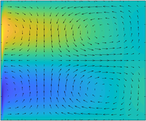
  $\unicode[STIX]{x1D702}$-values by continuation methods. The initial scan revealed that the fastest-growing mode can have a different form in different parts of the parameter space. For example, at $\unicode[STIX]{x1D702}\geqslant 0.5$ a mode in which $|u_{r}(r)|$ has a single maximum in $r$ usually dominates, whereas at small $\unicode[STIX]{x1D702}$ and $Fr<1$ the fastest-growing mode can have an eigenfunction in which $|u_{r}(r)|$ has many maxima.
We explored numerically only within the domain  $0.05\leqslant \unicode[STIX]{x1D702}\leqslant 0.95$, $0.05\leqslant \unicode[STIX]{x1D707}\leqslant 0.95$. When the Rayleigh stability criterion is not satisfied, the large $k$ inviscid modes are the fastest-growing modes (Billant & Gallaire Reference Billant and Gallaire2005). While the present work does examine both inviscid and viscous modes, we are primarily interested in the region of the parameter space where the two can be compared. We have therefore not explored very high $k$ inviscid modes in detail. Our solver has successfully reproduced numerical results from Shalybkov & Rüdiger (Reference Shalybkov and Rüdiger2005) and Le Dizès & Riedinger (Reference Le Dizès and Riedinger2010). It has also produced numerical results which mirror the low- $Re$ experimental results of Ibanez et al. (Reference Ibanez, Swinney and Rodenborn2016).
3 Sufficient conditions for WKBJ-inviscid SRI
As noted in § 1, we need to supplement our numerical results with an extension of the WKBJ analysis of Park & Billant (Reference Park and Billant2013). That analysis is based on taking  $k\gg 1$ and $m$ finite in (2.9), thus discarding all the terms within square brackets except the first, the term in $k^{2}$. The eigenfunctions governed by (2.9) then have scales much smaller than the gap width, with either exponential or oscillatory radial structure according to the sign of the term in $k^{2}$, which in turn depends on the configuration of the significant surfaces. Thus there can be WKBJ turning points at some of those surfaces, as for instance between a Kelvin wave with exponential structure near the inner boundary and an inertia–gravity wave with oscillatory structure further out, as in some cases of the RI.
When referring to an instability found in this way, we call it a WKBJ-inviscid SRI mode, to distinguish it from an inviscid SRI mode found numerically, which might have a value of  $k$ too low to justify the WKBJ approximations. Park & Billant (Reference Park and Billant2013) showed that for all $\unicode[STIX]{x1D707}\neq 1$ with $\unicode[STIX]{x1D707}\geqslant \unicode[STIX]{x1D702}^{2}$ there is WKBJ-inviscid SRI whenever the following conditions (3.1a,b) and (3.2) are both satisfied
 $$\begin{eqnarray}2\sqrt{\frac{\unicode[STIX]{x1D707}-\unicode[STIX]{x1D702}^{2}}{1-\unicode[STIX]{x1D702}^{2}}}<\frac{1}{Fr}\quad \text{if }\unicode[STIX]{x1D707}<1;\quad 2\sqrt{\frac{\unicode[STIX]{x1D707}(\unicode[STIX]{x1D707}-\unicode[STIX]{x1D702}^{2})}{1-\unicode[STIX]{x1D702}^{2}}}<\frac{1}{Fr}\quad \text{if }\unicode[STIX]{x1D707}>1,\end{eqnarray}$$
 $$\begin{eqnarray}\frac{2}{|1-\sqrt{\unicode[STIX]{x1D707}}|}\sqrt{\frac{\unicode[STIX]{x1D707}-\unicode[STIX]{x1D702}^{2}}{1-\unicode[STIX]{x1D702}^{2}}}<m<\frac{2}{Fr|1-\unicode[STIX]{x1D707}|}.\end{eqnarray}$$
 These therefore are sufficient conditions for the occurrence of WKBJ-inviscid instabilities, and they show that such instabilities will be found for any combination of  $(\unicode[STIX]{x1D702},\unicode[STIX]{x1D707})$ with $\unicode[STIX]{x1D707}\neq 1$ whenever $Fr$ is small enough, i.e. whenever the stratification is strong enough.
The value of  $m$ in (3.2) must be a positive integer. If
 $$\begin{eqnarray}\frac{2}{|1-\sqrt{\unicode[STIX]{x1D707}}|}\sqrt{\frac{\unicode[STIX]{x1D707}-\unicode[STIX]{x1D702}^{2}}{1-\unicode[STIX]{x1D702}^{2}}}+1<\frac{2}{Fr|1-\unicode[STIX]{x1D707}|}\end{eqnarray}$$
 then there must be a positive integer  $m$ satisfying (3.2), because (3.3) says that the right-hand side of (3.2) exceeds the left-hand side by at least 1, leaving room for at least one integer value of $m$ in between.
Of course these instability criteria (3.1a,b)–(3.3) cannot hold for the viscous domain because, in the limit  $k\gg 1$ with $Re$ fixed, all modes are stabilised by viscosity.
We note that any Kelvin-wave-mediated SRI, or other mode involving counterpropagating waves, must by virtue of that fact satisfy  ${\mathcal{R}}[\unicode[STIX]{x1D6F7}]=0$ somewhere in the flow so that the Lagrangian angular phase speeds $m^{-1}{\mathcal{R}}[\unicode[STIX]{x1D6F7}]$ have opposite signs at the inner and outer boundaries. Park & Billant (Reference Park and Billant2013) showed moreover that for any WKBJ-inviscid SRI at sufficiently small $Fr$ there is a radial interval within the flow within which the value of ${\mathcal{R}}[\unicode[STIX]{x1D6F7}]$ is enclosed by the inertia-wave epicyclic frequencies $\pm \sqrt{2Z\unicode[STIX]{x1D6FA}}$; see their figures 3 and 11. This comes about because their WKBJ-inviscid SRIs are mediated by inertia–gravity waves.
We now focus on the case  $0<\unicode[STIX]{x1D707}<1$ for the rest of the paper, leaving the interesting cases $\unicode[STIX]{x1D707}<0$ and $\unicode[STIX]{x1D707}>1$ for future work. In appendix A we show that if $Fr\leqslant 0.5$, then (3.1a) and (3.3) are satisfied for all $\unicode[STIX]{x1D707}$ in the range $\unicode[STIX]{x1D702}^{2}\leqslant \unicode[STIX]{x1D707}<1$. Since we know that inviscid axisymmetric modes are Rayleigh unstable for $\unicode[STIX]{x1D707}<\unicode[STIX]{x1D702}^{2}$, this gives the remarkable result that for $Fr\leqslant 0.5$ there is inviscid instability throughout the range $0<\unicode[STIX]{x1D702}<1$ and $0<\unicode[STIX]{x1D707}<1$.
The case  $\unicode[STIX]{x1D702}^{2}<\unicode[STIX]{x1D707}<1$ and $0.5<Fr\leqslant 2$ is more complicated, and the most useful sufficient conditions for WKBJ-inviscid instability are found by evaluating the $\unicode[STIX]{x1D707}$-values that satisfy (3.1a) and (3.3) numerically, as done in the $Fr=1$ case in § 4 below. However, in appendix A we derive inequalities showing that if
 $$\begin{eqnarray}\sqrt{\unicode[STIX]{x1D707}}<\sqrt{\frac{2}{Fr}}-1,\quad 0.5<Fr\leqslant 2\end{eqnarray}$$
 then there is WKBJ-inviscid instability for all values  $\unicode[STIX]{x1D702}$ satisfying $\unicode[STIX]{x1D702}^{2}<\unicode[STIX]{x1D707}$. In the limit $\unicode[STIX]{x1D702}\rightarrow 0$, (3.4) is a tight inequality, meaning that it gives the same maximum value of $\unicode[STIX]{x1D707}$ as the numerical solution of (3.1a) and (3.3) (see appendix A for details). For larger values of $\unicode[STIX]{x1D702}$ in the range $0<\unicode[STIX]{x1D702}<\sqrt{\unicode[STIX]{x1D707}}$, (3.4) still guarantees WKBJ-inviscid instability, but it is less useful because the maximum value of $\unicode[STIX]{x1D707}$ for the WKBJ-inviscid instability, as defined by (3.1a) and (3.3), is above the range given by (3.4).
The case of weak stratification,  $Fr>2$, is simpler to understand. In appendix A we show that if $\unicode[STIX]{x1D702}<\sqrt{1-2/Fr}$ then (3.3) cannot be satisfied, and WKBJ-inviscid SRI can only be guaranteed when $\unicode[STIX]{x1D707}<\unicode[STIX]{x1D702}^{2}$. If $\unicode[STIX]{x1D702}>\sqrt{1-2/Fr}$, there is a very thin wedge of $\unicode[STIX]{x1D707}>\unicode[STIX]{x1D702}^{2}$ where WKBJ-inviscid SRI occurs (i.e. (3.1a) and (3.3) are both satisfied) but is Rayleigh stable. However, this wedge is very thin. For example, in the case $Fr=10/3$ and $\unicode[STIX]{x1D702}=\sqrt{0.7825}=0.8846$ the range of $\unicode[STIX]{x1D707}$ where (3.1a) and (3.3) are satisfied is only $0.7825<\unicode[STIX]{x1D707}<0.7848$ (see equation (A 16) of appendix A). All other values of $\unicode[STIX]{x1D702}$ give an even smaller range of unstable $\unicode[STIX]{x1D707}$. So for $Fr=10/3$ and $\unicode[STIX]{x1D702}=0.8846$, $\unicode[STIX]{x1D707}<0.7825$ gives centrifugal instability, while $\unicode[STIX]{x1D707}>0.7848$ gives neither centrifugal instability nor WKBJ-inviscid SRI. However, as already mentioned, the WKBJ analysis (a) gives sufficient, not necessary, conditions for WKBJ-inviscid SRI, and (b) says nothing about non-WKBJ inviscid instabilities at moderate $k$. Indeed, such non-WKBJ instabilities will be encountered in the next section, well outside the thin wedge.
4 Domain of instability
Figure 1 shows the extent of instabilities determined numerically, viscous (‘○’ symbols) and inviscid (‘ $\times$’ symbols), for four values of $Fr$, varying from a weakly stratified case at $Fr=10/3$ to a strongly stratified case at $Fr=0.2$. These results were attained by use of a brute-force computational search for unstable modes throughout the parameter space of $(\unicode[STIX]{x1D702},\unicode[STIX]{x1D707},m,k)$. The approach described in § 2.3 was used to perform these searches.

Figure 1. Cases (a)  $Fr=10/3$, (b) $Fr=1$, (c) $Fr=0.5$, (d) $Fr=0.2$; arranged in order of increasing stratification. These plots display the inviscid and viscous unstable modes found for $0<\unicode[STIX]{x1D702}<1$ and $0<\unicode[STIX]{x1D707}<1$. Here, ‘ $\times$’ represents locations where we have found inviscid instabilities with growth rate above $10^{-5}$; ‘○’ represents locations that are viscously unstable for Reynolds numbers of $Re=10^{6}$ or less. The grey shaded region in each plot denotes where the flow is centrifugally unstable, $\unicode[STIX]{x1D707}<\unicode[STIX]{x1D702}^{2}$. The red shaded region on all four plots shows where WKBJ-inviscid SRI occurs according to (3.1a) and (3.3) with $\unicode[STIX]{x1D707}\geqslant \unicode[STIX]{x1D702}^{2}$. In (a) the red region is a very thin sliver (so thin we have had to thicken it here to improve visibility) that terminates in cusps at $(\unicode[STIX]{x1D702},\unicode[STIX]{x1D707})=(\sqrt{0.4},0.4)$ and $(\unicode[STIX]{x1D702},\unicode[STIX]{x1D707})=(1,1)$ (see the end of appendix A for details). Note that in (c,d) the entire domain of $\unicode[STIX]{x1D707}<1$ is predicted to be inviscidly unstable.
The grey region in each panel of figure 1 denotes the range of inviscid instability as predicted for  $k\gg 1$ by the Rayleigh criterion $\unicode[STIX]{x1D707}<\unicode[STIX]{x1D702}^{2}$. The red region denotes the range of WKBJ-inviscid instability as predicted by (3.1a) and (3.3), with finite growth rates on the Rayleigh neutral stability curve $\unicode[STIX]{x1D707}=\unicode[STIX]{x1D702}^{2}$. The very thin sliver of red in figure 1(a) terminates in cusps at $(\unicode[STIX]{x1D702},\unicode[STIX]{x1D707})=(\sqrt{0.4},0.4)$ and at $(\unicode[STIX]{x1D702},\unicode[STIX]{x1D707})=(1,1)$, and as remarked at the end of § 3 intersects the vertical line $\unicode[STIX]{x1D702}=0.8846$ in only a tiny interval $0.7825<\unicode[STIX]{x1D707}<0.7848$. This thin sliver of red has actually been thickened in figure 1(a) to improve visibility (see caption).
In figure 1(c,d), and in all similar plots for  $Fr\leqslant 0.5$, the results summarised in § 3 show that the grey and red regions together occupy the entire plot. That is, everywhere in these plots we have WKBJ-inviscid instabilities, either centrifugal (grey) or SRI (red). However, our numerical search has not found any instabilities in the top left corners of figure 1(c,d), the regions devoid of ‘○’ or ‘ $\times$’ symbols, despite much effort to search thoroughly. In the inviscid case, our solvers failed to find instabilities in these corners for one or both of two likely reasons, the first being that the instabilities may have ultra-low growth rates $\unicode[STIX]{x1D70E}$, below our chosen threshold $10^{-5}$, and second that they may exist only in tiny windows of $k$-space not intersected by the numerical search. In the viscous case, our search went up to $Re=10^{6}$ only, so it is possible that there are viscous instabilities in the top left corners of figure 1(c,d) at values of $Re$ too high for us to reach by numerical exploration.
There is a similar lack of numerical solutions for instabilities in the top left corners of figure 1(a,b). We did, on the other hand, find non-WKBJ inviscid instabilities, with modest  $k$ values, not only in the red and grey regions, but also to the left of the red regions at $\unicode[STIX]{x1D702}$ and $\unicode[STIX]{x1D707}$ values shown by the ‘ $\times$’ symbols. We suspect that some instabilities may again have been missed, but we are confident of each unstable result that we have found.
In figure 1(a,b) there are regions that are inviscidly stable but viscously unstable, marked by the ‘○’ symbols with no accompanying ‘ $\times$’. The largest such region, in figure 1(a), includes an overhang region between $0.4<\unicode[STIX]{x1D707}<0.6$. Its boundary moves to lower $\unicode[STIX]{x1D702}$ as $\unicode[STIX]{x1D707}$ increases. As this overhang boundary is approached from the right, for instance by reducing $\unicode[STIX]{x1D702}$ at constant $\unicode[STIX]{x1D707}$, the growth rates and $k$-windows of the non-WKBJ inviscid instabilities marked by ‘ $\times$’ symbols shrink to zero, and $\unicode[STIX]{x1D6F7}(r_{in})$ becomes real and equal to $-N$, a significant surface of (2.9) that is also a singular surface. A similar phenomenon in which inviscid instabilities disappear as this singular condition is approached was noted by Riedinger et al. (Reference Riedinger, Le Dizès and Meunier2010). When viscosity is added, the singular behaviour is removed and smooth regular viscous solutions are found as indicated by the ‘○’ symbols with no accompanying ‘ $\times$’ symbols.
There are precedents for viscosity being required for shear flow instabilities. For example, plane Poiseuille flow is stable in the inviscid domain, but unstable when the viscosity is non-zero (Drazin & Reid Reference Drazin and Reid1981). Another classic example is that of Tollmien–Schlicting and similar boundary-layer instabilities, e.g. Baines, Majumdar & Mitsudera (Reference Baines, Majumdar and Mitsudera1996). Recently, Ibanez et al. (Reference Ibanez, Swinney and Rodenborn2016) performed SRI experiments which showed that higher Reynolds numbers can stabilise the flow compared to unstable results at lower Reynolds numbers.
5 Critical viscous mode analysis
5.1 Critical viscous mode regions
In this section, we focus on  $Fr=1$ and explore the eigenfunction shapes of the critical viscous modes throughout the $(\unicode[STIX]{x1D702},\unicode[STIX]{x1D707})$-parameter space. We also explore the parameter space near to each critical viscous mode, seeking the neutral curves where modes transition from stable to unstable. These viscous $(m,k,Re)$ results are then compared to unstable modes found in the corresponding inviscid $(m,k)$-parameter space, in order to examine the connections and differences between the viscous and inviscid systems.
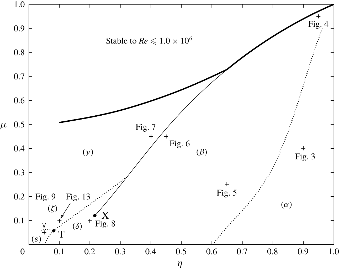
Figure 2. The different regions of the parameter space dependent upon the form of the critical viscous mode at each point for  $Fr=1$ are shown. The thick solid curve denotes the stability limit for modes with a Reynolds number below $Re=10^{6}$. The thin solid curve denotes a discontinuous change in the critical Reynolds number $Re_{c}$ of the instability mode. Dotted curves denote where the structure and wavenumbers of the critical viscous mode of instability discontinuously change, but $Re_{c}$ is continuous. These dotted curves are the boundaries between the different types of mode, and are curves where two different modes onset at the same critical Reynolds number. We do not denote changes of $m$ for $m>1$, which do not appear to significantly alter the eigenfunction structure, and were mostly seen only close to the narrow-gap limit of $\unicode[STIX]{x1D702}\rightarrow 1$. Regions $\unicode[STIX]{x1D6FC}$– $\unicode[STIX]{x1D701}$ are labelled and are discussed in the main text, as is the ‘point of continuity’ X which terminates the thin solid discontinuity curve. The point T at $\unicode[STIX]{x1D702}=0.081617$, $\unicode[STIX]{x1D707}=0.057637$ is the triple point where the three modes of instability corresponding to regions $\unicode[STIX]{x1D6FF}$, $\unicode[STIX]{x1D700}$ and $\unicode[STIX]{x1D701}$ all onset at the same critical Reynolds number, $Re_{c}=17\,493$. Each $+$ sign denotes the location of an example mode from the later figures within this paper.
Figure 2 shows the distinct critical viscous mode regions throughout the  $(\unicode[STIX]{x1D702},\unicode[STIX]{x1D707})$-parameter space for $Fr=1.0$. We have labelled the different critical viscous mode regions as $\unicode[STIX]{x1D6FC}$– $\unicode[STIX]{x1D701}$. They correspond to eigenfunctions with different shapes to be illustrated in figures 3–9 and 13.
The boundary between where the axisymmetric and non-axisymmetric modes have the lowest  $Re_{c}$ values, i.e. the boundary between regions $\unicode[STIX]{x1D6FC}$ and $\unicode[STIX]{x1D6FD}$, is somewhat to the right of the Rayleigh neutral stability curve $\unicode[STIX]{x1D707}=\unicode[STIX]{x1D702}^{2}$. Stratification delays the onset of centrifugal instability to higher $Re_{c}$ closer to that curve.
The thin solid curve in figure 2 will be called the ‘discontinuity curve’ because it marks a jump in the properties of the viscous critical mode, both in its shape and in its values of  $Re_{c}$ and $k$. This jump in $Re_{c}$ is associated with the restabilisation phenomenon, whereby the flow restabilises as the Reynolds number is increased beyond the first instability point. This phenomenon was noticed theoretically by Leclercq et al. (Reference Leclercq, Nguyen and Kerswell2016) and Rüdiger et al. (Reference Rüdiger, Seelig, Schultz, Gellert, Egbers and Harlander2017), and experimentally by Ibanez et al. (Reference Ibanez, Swinney and Rodenborn2016). The jump in properties is described in §§ 6.2–6.3 below. The jump disappears at the point X at the end of the discontinuity curve, beyond which the properties change continuously. This occurs because the critical viscous modes of the two regimes begin to overlap within the $(m,k,Re)$-parameter space, taking the form of an ‘inviscid-type’ SRI mode, by which is meant a viscous mode at high $Re$ whose eigenfunction shape strongly resembles that of an inviscid mode, apart from thin boundary layers, and whose wavenumber values are similar. We refer to X as the point of continuity; it is discussed further in § 6.3.
As already mentioned, region  $\unicode[STIX]{x1D6FC}$ has critical viscous modes that are classical centrifugal modes with $m=0$. Figure 3(a,b) shows a typical example, corresponding in figure 2 to the ‘ $+$’ symbol marked ‘figure 3’. Following Leclercq et al. (Reference Leclercq, Nguyen and Kerswell2016), we call region $\unicode[STIX]{x1D6FC}$ the centrifugal instability (CI) region. See § 5.2 below for more information on the figure captions. Region $\unicode[STIX]{x1D6FD}$ has preferred critical viscous modes that are SRIs with $m\neq 0$. Their eigenfunction shapes suggest mediation by inertia–gravity waves having broad radial structures, as in figures 4(a,b)–6(a,b). Again see the $+$ symbols in figure 2.
The three regions  $\unicode[STIX]{x1D6FF}$, $\unicode[STIX]{x1D700}$ and $\unicode[STIX]{x1D701}$ in figure 2 all meet at the triple point marked T in figure 2, marking a codimension-3 bifurcation, where three different viscous modes onset at the same critical Reynolds number, $Re_{c}=17\,493$, but with different $\unicode[STIX]{x1D714}$ and different critical $k$. For the $\unicode[STIX]{x1D6FF}$-region mode, $\unicode[STIX]{x1D714}=0.12436$ and $k=18.65$, for the $\unicode[STIX]{x1D700}$-region mode, $\unicode[STIX]{x1D714}=0.58340$ and $k=8.644$ and for the $\unicode[STIX]{x1D701}$-region mode, $\unicode[STIX]{x1D714}=0.57124$ and $k=77.93$. The corresponding eigenfunctions are illustrated in figures S13–S15 of the SI. For all three modes $m=1$. The dotted boundaries between regions $\unicode[STIX]{x1D6FF}$– $\unicode[STIX]{x1D700}$, $\unicode[STIX]{x1D700}$– $\unicode[STIX]{x1D701}$ and $\unicode[STIX]{x1D701}$– $\unicode[STIX]{x1D6FF}$ all mark codimension-2 boundaries, where two different modes onset simultaneously at the same $Re$. The modes in region $\unicode[STIX]{x1D701}$ near the triple point have a strong resemblance to the RI modes identified by Le Dizès & Riedinger (Reference Le Dizès and Riedinger2010) in the wide-gap limit of inviscid Taylor–Couette flow. An example of an RI-type critical viscous mode is shown in figure 13(a,b). Further from the triple point the radiating waves gradually disappear (see § 7.2) and the region $\unicode[STIX]{x1D701}$ modes then morph into inner boundary-trapped modes labelled $\unicode[STIX]{x1D6FE}$ in figure 2 and exemplified by figure 7(a,b) and SI figure S7. There is no definite boundary between the modes labelled $\unicode[STIX]{x1D6FE}$ and $\unicode[STIX]{x1D701}$ as the transition is gradual.
Region  $\unicode[STIX]{x1D6FF}$ corresponds to inviscid-type modes, as shown in figure 8(a,b). These modes have evolved from the region $\unicode[STIX]{x1D6FD}$ modes exemplified by figures 5(a,b) and 6(a,b). Again there is no definite boundary between the modes labelled $\unicode[STIX]{x1D6FD}$ and $\unicode[STIX]{x1D6FF}$. These modes also change their form gradually, so that in region $\unicode[STIX]{x1D6FD}$ the maximum amplitude is near the middle of the gap whereas in region $\unicode[STIX]{x1D6FF}$ the amplitude is largest near the inner cylinder wall (compare figures 4–6 and 8 below).
Finally in region  $\unicode[STIX]{x1D700}$, at the bottom left of figure 2, the wide gap suggests we should find modes that are even more RI-like. Instead, and perhaps surprisingly, we see critical viscous modes like that illustrated in figure 9, with broad radial structures and hints of outer boundary trapping. However, the configuration of significant surfaces, with ${\mathcal{R}}[\unicode[STIX]{x1D6F7}]=\pm N$ outside the flow while ${\mathcal{R}}[\unicode[STIX]{x1D6F7}]=0$ and ${\mathcal{R}}[\unicode[STIX]{x1D6F7}]=\pm \sqrt{2Z\unicode[STIX]{x1D6FA}}$ are all within the flow and close to the inner boundary, suggests instead that most of the domain, away from the inner boundary, is occupied by an inertia–gravity wave with a standing-wave radial structure, i.e. boundary reflected rather than boundary trapped. However, the shapes of the neutral curves show that this is another case of restabilisation as $Re$ increases. It seems that in order to phase lock together, the counterpropagating wave structures need to be modified by viscosity in a crucial way. We call these ‘wide-gap’ SRIs. They are preferred (having the lowest $Re_{c}$) only when $\unicode[STIX]{x1D702}<0.081617$.
The critical viscous modes in regions  $\unicode[STIX]{x1D6FE}$ and $\unicode[STIX]{x1D700}$ (figures 7 and 9) have no inviscid counterparts, i.e. they are not inviscid-type. They also exhibit restabilisation. By contrast, at least some of the critical viscous modes in region $\unicode[STIX]{x1D6FF}$ are inviscid-type as can be seen from the example in figure 8, which has $m=1$ and $k=9.07$ and is close to an inviscid mode with $m=1$ and maximum growth rate at $k=8.61$. Critical viscous RI modes in region $\unicode[STIX]{x1D701}$ can also have inviscid counterparts, see § 7.2 below.
5.2 Example figures
Figures 3 to 9 show examples of the eigenfunction shapes of critical viscous modes from each region alongside wavenumber analyses. Figure 13 shows examples of RI, discussed in § 7.2 below.
Each figure examines specific values of  $\unicode[STIX]{x1D702}$, $\unicode[STIX]{x1D707}$ and $Fr$. The critical $(m,k)$-wavenumbers and critical Reynolds numbers $Re_{c}$ are quoted in each figure. For each figure we also declare whether any of the following significant surfaces occur within the flow: ${\mathcal{R}}[\unicode[STIX]{x1D6F7}(r_{c})]=0$, or ${\mathcal{R}}[\unicode[STIX]{x1D6F7}(r_{\pm })]=\pm \sqrt{2Z\unicode[STIX]{x1D6FA}}$. These surfaces are relevant to the inviscid instability criteria of Park & Billant (Reference Park and Billant2013); see § 3. The significant surfaces ${\mathcal{R}}[\unicode[STIX]{x1D6F7}]=\pm N$ are absent in all our examples except for figure 13(c,d).
Each of figures 3–9 features four panels labelled (a–d): vertical (a) and horizontal (b) cross-sectional contour plots of the critical viscous mode of instability are shown. For the vertical cross-section (a) at  $\unicode[STIX]{x1D703}=0$, radial $u_{r}$ and vertical $u_{z}$ velocities are shown as vectors, whereas the azimuthal velocity $u_{\unicode[STIX]{x1D703}}$ perturbation is shown in colour contours. For the horizontal cross-section (b) at $z=0$, radial $u_{r}$ and azimuthal $u_{\unicode[STIX]{x1D703}}$ velocities are shown as vectors and the vertical velocity $u_{z}$ is shown in colour contours. The contours of both (a) and (b) use the same colour scale, $u_{i}/||u_{r}||$. The term $u_{i}$ represents $u_{\unicode[STIX]{x1D703}}$ or $u_{z}$ depending on which figure is being considered, while $||u_{r}||$ denotes the maximum radial velocity $u_{r}$ within the eigenmode, which we have chosen as our normalisation for these plots. Basic state flow is always in the positive $\unicode[STIX]{x1D703}$ direction. Each cross-section is taken over a sufficient range to demonstrate the full wavelength of each mode.
Except for figure 13, where (c) and (d) have the same form as (a) and (b), neutral curves of critical viscous stability at given a given  $k$ are shown in plot (c), for various values of $m$. The region below each curve is always stable. In some cases, the stable region also extends above a neutral curve, as with some of the curves in figure 6 onward, showing the restabilisation phenomenon as $Re$ increases. The critical viscous mode is marked on these plots with a cross $\boldsymbol{\times }$. The azimuthal wavenumber $m$ of each curve is labelled. Panel (d) shows growth rates $\unicode[STIX]{x1D70E}$ for inviscid instabilities, as functions of $k$ for various values of $m$. Each line colour corresponds to the same values of $m$ as in the viscous panel (c). We sometimes see a strong correlation between the bands of unstable inviscid wavenumbers compared to the sets of viscous wavenumbers that are unstable, but this is not always the case. In most cases, only the range $m=[0,1,2,3]$ is displayed. However, for figure 4 the relevant critical viscous mode has $m=7$, hence for that case we plot the inviscid modes for the range $m=[0,1,\ldots ,9]$.
6 Results and discussion
6.1 Eigenfunction shapes
Figure 3 is an example from region  $\unicode[STIX]{x1D6FC}$, the CI regime, where centrifugal instability is preferred. The vertical cross-section (a) exhibits strong azimuthal flow across the gap width, just as in the classical Taylor-vortex cell structure. CI are stabilised by the presence of stratification, increasing the critical Reynolds number compared to unstratified flow. The competition between the growth rate of CI compared with SRI is discussed by Leclercq et al. (Reference Leclercq, Nguyen and Kerswell2016). The $m=1$ neutral curve in figure 3(c) lies close to the $m=0$ curve, which is a feature of the classical (unstratified) Taylor-vortex problem, and we see from figure 2 that if $\unicode[STIX]{x1D702}$ is reduced slightly, past the dotted curve, the $m=1$ mode becomes preferred. Figure 3(d) shows that the inviscid modes stabilise at vertical wavenumber $k\approx 1$, consistent with the rapid increase in critical Reynolds number as $k$ approaches 1 seen in figure 3(c).
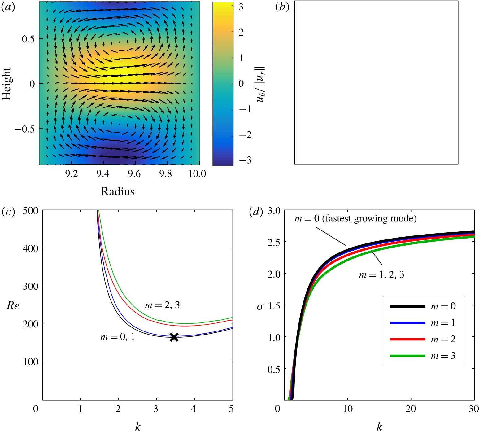
Figure 3. See § 5.2 for a description of the multiplot layout. An example of CI (centrifugal instability), found as the critical viscous mode within region  $\unicode[STIX]{x1D6FC}$ of figure 2. Here, $\unicode[STIX]{x1D702}=0.90$, $\unicode[STIX]{x1D707}=0.40$, and $Fr=1.0$. The critical viscous mode of instability has $Re_{c}=164.80$ with $m=0,k=3.454$, and $\unicode[STIX]{x1D714}=0.4217$. Panel (b) is left blank since the mode is axisymmetric, and hence there is no variation in the $\unicode[STIX]{x1D703}$ direction. The viscous and inviscid plots are labelled as (c,d) to match the layout of figures 4–9.

Figure 4. See § 5.2 for a description of the multiplot layout. An example of critical viscous SRI close to the narrow-gap limit, found as the critical viscous mode within region  $\unicode[STIX]{x1D6FD}$ of figure 2. Here, $\unicode[STIX]{x1D702}=0.95$, $\unicode[STIX]{x1D707}=0.95$, and $Fr=1.0$. The critical viscous mode of instability has $Re_{c}=3060.3$ with $m=7,k=2.809$, and $\unicode[STIX]{x1D714}=6.8190$. For this frequency, ${\mathcal{R}}[\unicode[STIX]{x1D6F7}(r_{c})]=0$ occurs at $r_{c}=19.5$, although ${\mathcal{R}}[\unicode[STIX]{x1D6F7}(r_{\pm })]=\pm \sqrt{2Z\unicode[STIX]{x1D6FA}}$ does not occur within the radial range. Note that the most unstable inviscid mode with the largest growth rate occurs here for $m=27$, much higher than the $m$ of the critical viscous mode.

Figure 5. See § 5.2 for a description of the multiplot layout. Another example of critical viscous SRI, here for  $\unicode[STIX]{x1D702}=0.65,\unicode[STIX]{x1D707}=0.25$ and $Fr=1.0$, occupying region $\unicode[STIX]{x1D6FD}$ of figure 2. The critical viscous mode of instability has $Re_{c}=119.6$ with $m=1,k=4.208$, and $\unicode[STIX]{x1D714}=0.5246$. For this frequency, ${\mathcal{R}}[\unicode[STIX]{x1D6F7}(r_{c})]=0$ occurs at $r_{c}=2.332$. ${\mathcal{R}}[\unicode[STIX]{x1D6F7}(r_{\pm })]=\pm \sqrt{2Z\unicode[STIX]{x1D6FA}}$ cannot occur for this $(\unicode[STIX]{x1D702},\unicode[STIX]{x1D707})$ because $2Z\unicode[STIX]{x1D6FA}<0$ throughout the radial range.

Figure 6. See § 5.2 for a description of the multiplot layout. Another example of critical viscous SRI, here for  $\unicode[STIX]{x1D702}=0.45,\unicode[STIX]{x1D707}=0.45$ and $Fr=1.0$, occupying region $\unicode[STIX]{x1D6FD}$ of figure 2, close to the thin solid discontinuity curve dividing region $\unicode[STIX]{x1D6FD}$ from region $\unicode[STIX]{x1D6FE}$. The critical viscous mode of instability has $Re_{c}=304.1$ with $m=1,k=4.436$ and $\unicode[STIX]{x1D714}=0.5951$. For this frequency, ${\mathcal{R}}[\unicode[STIX]{x1D6F7}(r_{c})]=0$ occurs at $r_{c}=1.273$, although ${\mathcal{R}}[\unicode[STIX]{x1D6F7}(r_{\pm })]=\pm \sqrt{2Z\unicode[STIX]{x1D6FA}}$ does not occur within the radial range. There is a closed unstable domain in the bottom left corner of (c), which is shown in more detail in figure 10(c). This closed domain contains the critical viscous mode of instability, but there is also a separate domain of instability visible for higher Reynolds numbers, which appears to be unbounded in $Re$.
$Re$.

Figure 7. See § 5.2 for a description of the multiplot layout. An example of the inner boundary-trapped SRI, found as the critical viscous mode within region  $\unicode[STIX]{x1D6FE}$ of figure 2. Here, $\unicode[STIX]{x1D702}=0.40,\unicode[STIX]{x1D707}=0.45$ and $Fr=1.0$. The critical viscous mode of instability has $Re_{c}=6526.7$ with $m=1,k=10.407$ and $\unicode[STIX]{x1D714}=0.7823$. For this frequency, ${\mathcal{R}}[\unicode[STIX]{x1D6F7}(r_{c})]=0$ occurs at $r_{c}=0.816$, although ${\mathcal{R}}[\unicode[STIX]{x1D6F7}(r_{\pm })]=\pm \sqrt{2Z\unicode[STIX]{x1D6FA}}$ does not occur within the radial range. An alternative view of the eigenfunction shape is given in SI figure S7.

Figure 8. See § 5.2 for a description of the multiplot layout. An example of an inviscid-type SRI, found as the critical viscous mode within region  $\unicode[STIX]{x1D6FF}$ of figure 2. Note that near the outer boundary there is a maximum velocity perturbation amplitude equal to $u_{\unicode[STIX]{x1D703}}=0.76$, (measured in units of the maximum radial velocity) and hence it is still significant compared to perturbations elsewhere in the flow. Here $\unicode[STIX]{x1D702}=0.20,\unicode[STIX]{x1D707}=0.10$ and $Fr=1.0$. The critical viscous mode of instability has $Re_{c}=670.1$ with $m=1,k=9.067$ and $\unicode[STIX]{x1D714}=0.2384$. For this frequency, ${\mathcal{R}}[\unicode[STIX]{x1D6F7}(r_{c})]=0$ occurs at $r_{c}=0.577$ and ${\mathcal{R}}[\unicode[STIX]{x1D6F7}(r_{-})]=-\sqrt{2Z\unicode[STIX]{x1D6FA}}$ occurs at $r_{-}=0.319$. ${\mathcal{R}}[\unicode[STIX]{x1D6F7}(r_{+})]=+\sqrt{2Z\unicode[STIX]{x1D6FA}}$ does not occur within the radial range.

Figure 9. See § 5.2 for a description of the multiplot layout. An example of the wide-gap SRI, found as the critical viscous mode within region  $\unicode[STIX]{x1D700}$ of figure 2. Here, $\unicode[STIX]{x1D702}=0.05,\unicode[STIX]{x1D707}=0.05$ and $Fr=1.0$. The critical viscous mode of instability has $Re_{c}=20\,008$ with $m=1$, $k=9.477$, and $\unicode[STIX]{x1D714}=0.5378$. For this frequency, ${\mathcal{R}}[\unicode[STIX]{x1D6F7}(r_{c})]=0$ occurs at $r_{c}=0.0734$, ${\mathcal{R}}[\unicode[STIX]{x1D6F7}(r_{-})]=-\sqrt{2Z\unicode[STIX]{x1D6FA}}$ occurs at $r_{-}=0.0536$, and ${\mathcal{R}}[\unicode[STIX]{x1D6F7}(r_{+})]=+\sqrt{2Z\unicode[STIX]{x1D6FA}}$ occurs at $r_{+}=0.102$. Note that the range of inviscidly unstable wavenumbers appears to be entirely distinct from the range of viscously unstable wavenumbers.
Figures 4–6 present examples from region  $\unicode[STIX]{x1D6FD}$. Here, the critical viscous modes are SRIs with eigenfunctions similar to those seen in Shalybkov & Rüdiger (Reference Shalybkov and Rüdiger2005). They have simple eigenfunction shapes, filling the gap, with length scales of the same order as the gap width, in this respect like CI modes. We label them ‘simple SRI’. As already mentioned, the cross-sections in figures 4(a,b)–6(a,b) hint at inertia–gravity wave structures. These are counterpropagating because ${\mathcal{R}}[\unicode[STIX]{x1D6F7}]$ changes sign near the centre of the gap. The waves propagate against the mean flow on each side of the gap. For $Fr=1$, as in figures 4–6, the SRIs seen in region $\unicode[STIX]{x1D6FD}$ typically have $Re_{c}$ values in the range $100<Re_{c}<400$, although this increases as one approaches the narrow gap limit. For instance, $Re_{c}=3060.3$ in figure 4, which has $\unicode[STIX]{x1D702}=0.95$.
In the case of figure 4, the vertical structure of the critical SRI  $m=7$ mode is similar looking to that of the CI $m=0$ mode; compare figures 4(a) and 3(a). Notably this similarity is not seen for the inviscid eigenfunctions, suggesting that the viscous SRI has enabled Rayleigh-like behaviour to persist beyond the Rayleigh neutral curve, albeit for $m\neq 0$. The neutral curves in figure 4(c), corresponding to the various values of $m$, are all very close together – this is a phenomenon that occurs as the narrow-gap limit is approached, with the critical azimuthal wavenumber $m_{c}$ climbing to higher and higher values. A slight surprise is that the band of inviscidly unstable vertical wavenumbers is significantly narrower than the range of the viscously unstable wavenumbers, comparing figures 4(c) and 4(d).
Figure 5(a,b) shows an example of critical viscous SRI in the heart of the SRI region  $\unicode[STIX]{x1D6FD}$ of figure 2. The form of the instability is fairly similar to the narrow-gap case of figure 4, supporting the view that the instability mechanism is the same. Again we see Rayleigh-like behaviour in the vertical cross-section; compare figure 5(a) to figure 3(a). The radius at which ${\mathcal{R}}[\unicode[STIX]{x1D6F7}]=0$ has moved slightly inward from the midway position between the cylinders. We see from figure 5(c,d) that $m=0$ can still be unstable, because $\unicode[STIX]{x1D707}<\unicode[STIX]{x1D702}^{2}$, although $m=0$ is no longer the first mode to become unstable. For much of region $\unicode[STIX]{x1D6FD}$ of figure 2, CI and SRI are both active, it is just that the SRI mode tends to dominate at $Fr=1$ or less. Unlike the narrow-gap case, the lower bound of the range of inviscid unstable vertical wavenumbers is a good indicator of the form of the viscous neutral curve, compare figures 5(c) and 5(d).
Figure 5(d) has been cut off at  $k=30$. At these values of $\unicode[STIX]{x1D702}$ and $\unicode[STIX]{x1D707}$, inviscid instability is found at all large wavenumbers. For the $m=1$ mode, the growth rate increases monotonically with $k$, and at large $k$ the inviscid instability is concentrated near the inner cylinder (Billant & Gallaire Reference Billant and Gallaire2005). However, these high wavenumber unstable modes play no role in the viscous theory of onset, because they are strongly damped by viscosity.
Figures 6 and 7 are examples of SRI lying on either side of the boundary between regions  $\unicode[STIX]{x1D6FD}$ and $\unicode[STIX]{x1D6FE}$. Although these two points are nearby in parameter space there is a big difference in their $Re_{c}$. Figure 6 in region $\unicode[STIX]{x1D6FD}$ is another example of the simple viscous SRI mode, similar to figure 5 though with the instability enhanced near the inner cylinder compared to the outer. Figure 6(c) shows a strange behaviour, with a closed domain of instability at $Re\approx 300$ (see also figure 10c). Even a slight increase in $Re$ stabilises the system, though it becomes unstable again at larger $Re$. This behaviour is discussed in §§ 6.2 and 6.3 below. Figure 6(d) is very different from figure 5(d). The large wavenumber inviscid instability concentrated near the inner boundary disappears as we travel in parameter space across the Rayleigh neutral curve between $(\unicode[STIX]{x1D702},\unicode[STIX]{x1D707})=(0.65,0.25)$ and $(0.45,0.45)$ leaving only thin bands of inviscidly unstable wavenumbers. If $\unicode[STIX]{x1D702}$ is further reduced these thin bands of unstable wavenumbers disappear, consistent with figure 1(b).
Figure 7 is in region  $\unicode[STIX]{x1D6FE}$. There are two types of minimal- $Re$ mode in figure 7(c), which is similar to figure 6(c) apart from the disappearance of the closed unstable domain. The first of these modes is the critical viscous mode, marked with a cross in figure 7(c), with wavenumbers $m=1$ and $k=10.407$. This is the inner boundary-trapped mode shown in figure 7(a,b); see SI figure S7 for a more detailed view of the same mode. It has very little activity away from the inner boundary, hence the name inner boundary-trapped mode. If $\unicode[STIX]{x1D702}$ and $\unicode[STIX]{x1D707}$ are reduced, moving from the $\unicode[STIX]{x1D6FE}$-region to the $\unicode[STIX]{x1D701}$-region in figure 2, at around $\unicode[STIX]{x1D702}\approx \unicode[STIX]{x1D707}\approx 0.2$ the inner boundary-trapped mode morphs into an RI (see figures S1–S6 of the SI), like that in figures 13(a,b) below, where wave-like behaviour becomes apparent in the outer regions of the gap. The RI is further described in § 7.2 below.
As already remarked, the figure 7(a,b) mode is not inviscid-type. There is no inviscid mode resembling it, and it has no counterpart in figure 7(d). The figure 7(a,b) mode depends not only on viscosity but also, evidently, on the no-slip condition at the inner boundary, and in this respect it resembles the inherently viscous boundary-layer shear instability studied by Baines et al. (Reference Baines, Majumdar and Mitsudera1996).
The second minimal- $Re$ mode in figure 7(c), which has vertical wavenumber near $k\approx 5$ and onsets at $Re=71\,840$ (shown as figure S17 in the SI), does, by contrast, have an $m=1$ inviscid counterpart in figure 7(d). It has an eigenfunction (shown as figure S18 in the SI) resembling the viscous eigenfunction except close to the boundaries. So it qualifies as an inviscid-type mode as previously defined in § 5.1. There are counterpropagating waves trapped near each boundary, with velocity fields closely similar to the Kelvin waves noted by Kushner et al. (Reference Kushner, McIntyre and Shepherd1998) and Yavneh et al. (Reference Yavneh, McWilliams and Molemaker2001). If we reduce $\unicode[STIX]{x1D702}$ and $\unicode[STIX]{x1D707}$, moving down and to the left in figure 2, keeping to the left of the thin solid discontinuity curve – but now moving not toward region $\unicode[STIX]{x1D701}$ but toward region $\unicode[STIX]{x1D6FF}$, on the far side of the dotted curve – then the critical Reynolds number of the inviscid-type mode reduces faster than that of the inner boundary-trapped mode. Eventually the inviscid-type mode has a lower $Re_{c}$ than the inner boundary-trapped mode, so that the counterpart of figure 7(c) would have the inviscid-type mode on the left of figure 7(c) having a lower minimum than the inner boundary-trapped mode on the right. Thus when the dotted curve marking the $\unicode[STIX]{x1D6FE}$– $\unicode[STIX]{x1D6FF}$ border is crossed downward in figure 2, the inviscid-type mode, with its lower $k$ value, takes over from the inner boundary-trapped mode as the critical viscous mode. Note that in figure 7(d) the fastest-growing inviscid mode is the $m=2$ mode, but in the viscous mode picture, figure 7(c), it is the $m=1$ mode that has the lower critical $Re$, the $m=2$ viscous mode (not shown) having higher $Re$.
$Re$.
Figure 8 is typical of the inviscid-type mode found in region  $\unicode[STIX]{x1D6FF}$. Comparing figures 8(c) and 8(d) we see the first viscous mode to become unstable as $Re$ is raised, marked with a cross in figure 8(c), has a $k$ value, $k=9.067$, similar to that of the fastest-growing inviscid mode, as well as the same $m$ value, $m=1$. The inviscid mode eigenfunctions (shown in figure S21 of the SI) resemble the corresponding viscous eigenfunctions. So once again we have an inviscid-type mode as defined in § 5.1. Like the inner boundary-trapped modes in region $\unicode[STIX]{x1D6FE}$ in figure 2, the inviscid-type mode has a large amplitude near the inner boundary, but it still has significant amplitude near the outer boundary, particularly noticeable in the azimuthal velocity contours in figure 8(a). This distinguishes it from the inner boundary-trapped mode where there is essentially no activity near the outer boundary.
Figure 8(c) has a number of interesting features. In addition to the dominant inviscid and viscous modes with  $m=1$ and $k\approx 9$, the ‘overtone’ inviscid modes at $k\approx 17$ and $k\approx 23$ also show up on the viscous figure 8(c), though curiously the $k\approx 23$ viscous mode has ‘necked off’, generating a closed unstable domain similar to that seen in figure 6(c). These ‘overtone’ inviscid modes again have similar eigenfunctions to their corresponding viscous modes (not shown). There is an additional low- $k$ mode visible in figure 8(c) with $k\approx 3$. This mode has no inviscid counterpart, and its eigenfunctions look quite different from the mode shown in figure 8(a,b). This low- $k$ mode has strong activity right up to the outer boundary. At $Fr=1$ this low- $k$ mode is never the first to become unstable as $Re$ increases, so we have not plotted an example here. It is possible, however, that this mode (and indeed others not shown here) might become more significant at other values of $Fr$.
$Fr$.
When approaching region  $\unicode[STIX]{x1D700}$ from region $\unicode[STIX]{x1D6FF}$, moving toward the bottom-left corner of figure 2, there is another discontinuous change in the shape and vertical wavenumber of the critical viscous mode, although $Re_{c}$ remains continuous. This is represented by the short dotted curve separating the two regions in figure 2. Another short dotted curve in this figure separates region $\unicode[STIX]{x1D700}$ from region $\unicode[STIX]{x1D701}$ where again there is a change in eigenfunction form but no discontinuity in $Re$. Region $\unicode[STIX]{x1D700}$ exhibits a high- $Re$ SRI as the critical viscous mode, which we call the wide-gap mode, or wide-gap SRI. An example is shown in figure 9. Particularly striking are the strong vertical flows occupying most of the gap. This wide-gap mode and the radiative instability shown in figure 13 below could be related to the wall modes found in the non-rotating study of Chen, Bai & Le Dizés (Reference Chen, Bai and Le Dizés2016). For $Fr=1.0$ the wide-gap-mode SRI typically has a critical Reynolds number of $Re_{c}>10^{4}$. There are no inviscid unstable modes for the range of $k$ and $m$ for which we find wide-gap-mode SRI, so there is a lack of correlation here between the unstable wavenumbers of the viscous and inviscid systems. For this mode we see distinct bands of viscous instability within the $(m,k,Re)$-parameter space, as seen in figure 9(c). Inviscid-type modes, in the form of viscous modes corresponding to the high- $k$ inviscid modes in figure 9(d) were found, but are not shown as they onset at higher $Re$ than the wide-gap modes.
6.2 Closed unstable domains
Figure 10 shows examples of several closed unstable domains, like that already seen in figure 6(c). Figure 10(c) zooms in on the lower-left part of figure 6(c). These are closed regions of the  $(m,k,Re)$-parameter space for fixed values of $(\unicode[STIX]{x1D702},\unicode[STIX]{x1D707},Fr)$; here the flow can be made linearly unstable for a finite range of $Re$ only. Restabilisation always occurs when $Re$ is increased. A similar closed unstable domain phenomenon can be seen in the Taylor–Couette problem with vertical flow, see Cotrell & Pearlstein (Reference Cotrell and Pearlstein2004), Altmeyer, Hoffmann & Lücke (Reference Altmeyer, Hoffmann and Lücke2011). Viscosity is clearly important in the closed unstable domain phenomenon, and in a way that can be sensitive to parameter values. For instance, if $\unicode[STIX]{x1D702}$ is slightly reduced from 0.45 to 0.40, keeping $\unicode[STIX]{x1D707}=0.45$ – i.e. moving leftward across the thin discontinuity curve in figure 2 from the cross marked figure 6 to that marked figure 7 – we see a dramatic change in $Re_{c}$ from 304.1 to 6526.7 as the critical viscous mode changes shape and $k$-value. It has been verified that these changes are indeed discontinuous and take place precisely as the thin discontinuity curve is crossed, whether leftward or upward. It will be seen shortly that the changes are associated with the closed unstable domain disappearing – altogether ceasing to exist. By contrast, the co-existing inviscid modes have properties and fastest growth rates that vary smoothly across the discontinuity curve.

Figure 10. Examples of closed unstable domains. For flow parameters within these domains, the flow is linearly unstable, whereas it is stable outside. These therefore provide examples where increasing  $Re$ can restabilise the flow. (a) $\unicode[STIX]{x1D702}=0.56,\unicode[STIX]{x1D707}=0.50$ and $Fr=10/3$. (b) $\unicode[STIX]{x1D702}=0.57,\unicode[STIX]{x1D707}=0.50$ and $Fr=10/3$. (c) $\unicode[STIX]{x1D702}=0.45,\unicode[STIX]{x1D707}=0.45$ and $Fr=1$. (d) $\unicode[STIX]{x1D702}=0.70,\unicode[STIX]{x1D707}=0.70$ and $Fr=1$. All four panels have $m=1$.
Closed unstable domains are numerically challenging to find, as they are easily missed without a rigorous and time-consuming scan of the entire  $(m,k,Re)$-parameter space. In general we have found closed unstable domains only by utilising guesses from nearby regions of the $(\unicode[STIX]{x1D702},\unicode[STIX]{x1D707},Fr)$-parameter space.
In each case where we have observed closed unstable domains, some form of instability does appear to switch on again as  $Re$ is further increased, as happens in the case of figure 6(c). In that case, separate domains of instability can be seen at higher $Re$ in figure 6(c), with inviscid-type modes that morph continuously into inviscid modes as $Re\rightarrow \infty$. Such modes are seen for $m=2$ near $k\approx 4$, in figure 6(c), and for $m=1$ near $k\approx 4.4$. The latter may well be continuous with the $m=1$ mode near $k\approx 5$ in figure 7(c).
Regarding the closed unstable domains, in some cases we have evidence that they can quickly shrink, and then disappear, as parameters are changed within the  $(Re,Fr,\unicode[STIX]{x1D702},\unicode[STIX]{x1D707})$-parameter space. Consider figure 10(a,b), which shows closed unstable domains for slightly different $\unicode[STIX]{x1D702}$ values, 0.56 and 0.57, with $\unicode[STIX]{x1D707}=0.5$ and $Fr=10/3$. As can be seen, the closed domain at $\unicode[STIX]{x1D702}=0.56$ is significantly smaller, with a Reynolds number range of $700<Re<875$ rather than the range $600<Re<1175$ of $\unicode[STIX]{x1D702}=0.57$. Upon further reducing $\unicode[STIX]{x1D702}$, the closed unstable domain shrinks and ultimately disappears entirely.
Since the critical viscous mode in figure 6 is on the edge of a closed unstable domain, which disappears as  $\unicode[STIX]{x1D702}$ is decreased or $\unicode[STIX]{x1D707}$ is increased, the critical viscous mode must, as already remarked, jump discontinuously when the closed unstable domain ceases to exist. It changes its eigenfunction shape discontinuously, with an upward jump in $Re_{c}$. The discontinuous behaviour accounts for the way figures 6 and 7 differ so drastically, even though they are closely adjacent in parameter space, with $\unicode[STIX]{x1D702}$ values only 0.05 apart and $\unicode[STIX]{x1D707}$ values the same. At around $\unicode[STIX]{x1D702}=0.65$ and $\unicode[STIX]{x1D707}=0.72$, the upward jump in $Re_{c}$ takes $Re_{c}$ to values beyond the threshold stability limit $Re\leqslant 10^{6}$ set in the numerical search. That is where the thin discontinuity curve meets the thick solid stability limit curve in figure 2.
A similar closed unstable domain phenomenon is seen in figure 6 of Rüdiger et al. (Reference Rüdiger, Seelig, Schultz, Gellert, Egbers and Harlander2017). This figure, derived numerically, shows a closed unstable domain in the  $(Re,Rn)$-parameter space for $\unicode[STIX]{x1D702}=0.52$ and $m=1$. Here $Rn=Nr_{in}d/\unicode[STIX]{x1D708}$ is a stratification Reynolds number. This closed unstable domain disappears at around $\unicode[STIX]{x1D707}\simeq 0.571$, which is similar to our result (not shown here) of seeing the corresponding closed unstable domain disappear at $\unicode[STIX]{x1D707}\approx 0.58$ for $\unicode[STIX]{x1D702}=0.52$, $Fr=1$.
6.3 The point of continuity
As already mentioned in §§ 5.1 and 6.1, the thin solid curve in figure 2 marks a discontinuous jump in  $Re_{c}$ and other viscous SRI properties; and in § 6.2 we explained how this jump is related to the vanishing of closed unstable domains. As we reduce $\unicode[STIX]{x1D702}$ and $\unicode[STIX]{x1D707}$ along the thin solid discontinuity curve in figure 2, the jump becomes steadily smaller until the change in $Re_{c}$, and the other properties, becomes continuous at the point X. We called X the point of continuity; and for $Fr=1$ it is approximately at $\unicode[STIX]{x1D702}=0.2172$ and $\unicode[STIX]{x1D707}=0.1212$. Figure 11 shows how the discontinuity disappears (see caption).

Figure 11. Tracking the discontinuity in  $Re_{c}$ near to the point X in figure 2. Each plot shows the critical Reynolds number $Re_{c}$ for instability for a range of $\unicode[STIX]{x1D702}$ and $\unicode[STIX]{x1D707}$ values. In both plots we have $Fr=1.0$. We can see that the system transitions from continuous to discontinuous as $\unicode[STIX]{x1D702}$ and $\unicode[STIX]{x1D707}$ are increased. In (a), we have $0.2<\unicode[STIX]{x1D702}<0.25$. Blue crosses give the results for $\unicode[STIX]{x1D707}=0.11$, red pluses give the results for $\unicode[STIX]{x1D707}=0.12$ and green dots give the results for $\unicode[STIX]{x1D707}=0.14$. In (b), we have $0.1<\unicode[STIX]{x1D707}<0.15$. Blue crosses give the results for $\unicode[STIX]{x1D702}=0.21$, red pluses give the results for $\unicode[STIX]{x1D702}=0.22$ and green dots give the results for $\unicode[STIX]{x1D702}=0.23$.

Figure 12. (a) A plot of the  $(m,k,Re)$-parameter space for $\unicode[STIX]{x1D702}=0.22,\unicode[STIX]{x1D707}=0.1245,m=1$ and $Fr=1.0$, just above the point of continuity X in figure 2. It can be seen that the closed unstable domain of region $\unicode[STIX]{x1D6FD}$ has merged with the unbounded high- $Re$ domain of region $\unicode[STIX]{x1D6FF}$. (b) Neutral curves in $(k,Re)$-parameter space for $\unicode[STIX]{x1D702}=0.0786,\unicode[STIX]{x1D707}=0.05,m=1$ and $Fr=1.0$, at the transition between region $\unicode[STIX]{x1D6FF}$ and region $\unicode[STIX]{x1D700}$.
The point of continuity is a result of an overlap of the relevant domains in the viscous parameter space between the simple viscous SRI and the inviscid-type SRI. In figure 6(c) we see the  $m=1$ closed unstable domain at $k\approx 4.4$ with a critical $Re_{c}=304.1$, and an $m=1$ inviscid-type mode with a similar $k$ but a minimum $Re\approx 12\,000$, much larger. The closed unstable domain in figure 6(c) resembles a teardrop below the upper $m=1$ inviscid-type mode branch. If we look at the cross corresponding to figure 6 in figure 2, it lies just to the right of the thin discontinuity curve. As we move in $(\unicode[STIX]{x1D702},\unicode[STIX]{x1D707})$-parameter space downward and to the left, just keeping on the right-hand-side of the thin discontinuity curve, the minimum $Re$ value of the inviscid-type mode drops rapidly, while the $Re_{c}$ of the closed unstable domain mode varies only slowly. At a value of $\unicode[STIX]{x1D707}$ just above the point X value, and with $\unicode[STIX]{x1D702}$ just to the right of the discontinuity curve, the closed unstable domain teardrop has become smaller and hangs just below the curve corresponding to the inviscid-type neutral modes. If we keep $\unicode[STIX]{x1D707}$ fixed and reduce $\unicode[STIX]{x1D702}$, crossing the discontinuity curve, the teardrop closed unstable domain disappears, and $Re_{c}$ jumps up, but only by a small amount because the $Re_{c}$ corresponding to the inviscid-type mode was only just above the $Re_{c}$ of the closed unstable domain. If instead of crossing the discontinuity curve, we continue down and left in $(\unicode[STIX]{x1D702},\unicode[STIX]{x1D707})$-parameter space, passing to the right of X, the teardrop closed unstable domain is engulfed by the inviscid-type mode. A plot in the $(k,Re)$-parameter space of the neutral curve for a case near X, at $\unicode[STIX]{x1D702}=0.22$, $\unicode[STIX]{x1D707}=0.1245$, is shown in figure 12(a). So with a value of $\unicode[STIX]{x1D707}$ below that of point X in figure 2, no discontinuity in $Re_{c}$ occurs as $\unicode[STIX]{x1D702}$ is varied. Some more detailed information about closed unstable domains and the point of continuity is given in § 7 of the SI.
6.4 Wide-gap transition
The transition between regions  $\unicode[STIX]{x1D6FF}$ and $\unicode[STIX]{x1D700}$ does not involve closed unstable domains. Instead, as the transition is approached, the inviscid-type SRI of region $\unicode[STIX]{x1D6FF}$ requires increasingly high $Re_{c}$. At the same time, the wide-gap SRI becomes more unstable, with smaller $Re_{c}$. The two instabilities operate at different bands of vertical wavenumber $k$, and as the transition between the two regions is crossed, the wide-gap SRI becomes more unstable than the inviscid-type SRI. The transition between regions $\unicode[STIX]{x1D6FF}$ and $\unicode[STIX]{x1D700}$ can therefore be considered to be another codimension-2 bifurcation.
This transition can be seen in figure 12(b), which shows an example where the two instabilities have approximately the same  $Re_{c}$. In this figure, the wide-gap-mode SRI corresponds to the unstable region around $k\approx 9$, whereas the inviscid-type SRI corresponds to the unstable region around $k\approx 20$. Figure 12(b) corresponds to the point $(\unicode[STIX]{x1D702},\unicode[STIX]{x1D707})=(0.0786,0.05)$ in figure 2, on the dotted curve just below and to the left of the triple point T, which is at $(\unicode[STIX]{x1D702},\unicode[STIX]{x1D707})=(0.081617,0.057637)$. If we move slightly to the right of the dotted curve, by making $\unicode[STIX]{x1D702}$ slightly greater than 0.0786 keeping $\unicode[STIX]{x1D707}=0.05$, then the inviscid-type mode with higher $k$ onsets first. If instead we move slightly to the left, then the wide-gap mode onsets first.
Separate wavenumber bands of instability are predicted to exist for the viscous domain. In the present work they are seen only in figures 7(c), 8(c), 9(c) and 12(b); this is because we have generally provided a zoomed-in view of the local  $(m,k,Re)$-parameter space.
7 Radiative instability
7.1 Background
The radiative instability is a form of stratified non-axisymmetric instability characterised by the presence of a perturbation wave, strongest near the significant surface  ${\mathcal{R}}[\unicode[STIX]{x1D6F7}(r_{c})]=0$, close to the inner cylinder. It travels around the inner cylinder, with an outward propagating wave in the outer regions $r>r_{c}$ of the gap. Le Dizès & Riedinger (Reference Le Dizès and Riedinger2010) found WKBJ-inviscid RI when the outer cylinder had been moved to infinity, replacing the usual outer boundary condition with a condition allowing only outward radiation, which for a growing mode implies exponential decay with $r$ because the group velocity is finite (McIntyre & Weissman Reference McIntyre and Weissman1978). At weaker stratification, when a significant surface ${\mathcal{R}}[\unicode[STIX]{x1D6F7}(r)]=\pm N$ can occur, Le Dizès & Riedinger (Reference Le Dizès and Riedinger2010) found a form of RI in which the waves do not propagate all the way to the outer cylinder, but are truncated beyond this significant surface.
Experimental confirmation that RIs exist was provided by Riedinger et al. (Reference Riedinger, Le Dizès and Meunier2011). From the edge of the inner cylinder to the edge of their large rectangular tank, the smallest gap width was 17.5 times the radius of the largest cylinder used, roughly corresponding to  $\unicode[STIX]{x1D702}\leqslant 0.057$.
RI-like modes were detected in numerical viscous simulations by Leclercq et al. (Reference Leclercq, Nguyen and Kerswell2016) for non-wide-gap flows with  $\unicode[STIX]{x1D702}=0.417$. It was found for linear perturbations in the supercritical domain, i.e. beyond the onset of instability. They found a growing mode that had a significant surface with ${\mathcal{R}}[\unicode[STIX]{x1D6F7}(r_{c})]=0$ and wave-like behaviour at larger $r$. As in the Le Dizès & Riedinger (Reference Le Dizès and Riedinger2010) theory, the wave-like behaviour terminated beyond the significant surface where ${\mathcal{R}}[\unicode[STIX]{x1D6F7}(r)]=N$, see Leclerq et al. figure 7(a) and figure S16 of the SI. In the presence of viscosity this significant surface can act like a wave absorber. They found this behaviour at $Re=10^{6}$, $m=1$ and $\unicode[STIX]{x1D707}$ just below the Rayleigh critical value of $\unicode[STIX]{x1D702}^{2}$. The fastest-growing mode there has $k$ large, typically over $100$. This detection confirmed that the RI could exist away from the wide-gap limit, although it remained unclear whether the RI could exist as a critical viscous mode of instability. Examples where it does exist have been found in our work, as will be illustrated next.
7.2 The RI in the present work
Figure 13(a,b) gives an example of viscous RI that is also the critical viscous mode. It is the first mode to become unstable as  $Re$ increases, at $m=1$ and $k=54.72$, with $Re=Re_{c}=12565.1$. Here, $\unicode[STIX]{x1D702}=\unicode[STIX]{x1D707}=0.1$, close to the triple point $T$ in figure 2, lying in the $\unicode[STIX]{x1D701}$ region. At onset the significant surface with ${\mathcal{R}}[\unicode[STIX]{x1D6F7}(r_{c})]=0$ is close to the inner boundary, and the amplitude of the disturbance is greatest there. WKBJ-inviscid theory predicts there should be wave-like behaviour beyond the significant surface $r=r_{+}=0.2480$, where the Lagrangian frequency ${\mathcal{R}}[\unicode[STIX]{x1D6F7}]$ equals the epicyclic frequency $\sqrt{2Z\unicode[STIX]{x1D6FA}}$. Figure 13(a,b) shows that waves are indeed visible in the outer parts of the annulus beyond this significant surface for this critical viscous mode. The colour scheme has been altered in figure 13 from the previous scheme to make the relatively low amplitude waves more visible. As $N$ is greater than $|{\mathcal{R}}[\unicode[STIX]{x1D6F7}]|$ for all $r$, the significant surfaces ${\mathcal{R}}[\unicode[STIX]{x1D6F7}(r_{\pm })]=\pm N$ cannot occur in this $Fr=1$ case, and the waves reach the outer boundary. They are reflected back only weakly, thanks to the viscous attenuation and the finiteness of the group velocity, as can be seen from the very weak standing-wave pattern near the boundary. The $m=2$ mode has a local minimum over $Re$ at $k=96.49$ with $Re=39\,032$, larger than the $m=1$ critical value.

Figure 13. Two examples of the radiative instability as the critical viscous mode of instability for stratified Taylor–Couette flow, in region  $\unicode[STIX]{x1D701}$. (a,b) $\unicode[STIX]{x1D702}=\unicode[STIX]{x1D707}=0.1$, $m=1$, $Fr=1$. The critical viscous mode of instability has $Re_{c}=12565.1$ with $k=54.72$. The details of the contour plots are given in § 5.2. $\unicode[STIX]{x1D714}=0.5888$, ${\mathcal{R}}[\unicode[STIX]{x1D6F7}(r_{c})]=0$ at $r=0.1501$, ${\mathcal{R}}[\unicode[STIX]{x1D6F7}(r_{-})]=-\sqrt{2Z\unicode[STIX]{x1D6FA}}$ does not occur, but ${\mathcal{R}}[\unicode[STIX]{x1D6F7}(r_{+})]=\sqrt{2Z\unicode[STIX]{x1D6FA}}$ occurs at $r=0.2480$, and $\max (|\unicode[STIX]{x1D6F7}|)=0.4888<N=1$. (c,d) $\unicode[STIX]{x1D702}=\unicode[STIX]{x1D707}=0.1$, $m=1$, $Fr=2$. The critical viscous mode of instability has $Re_{c}=18016$ with $k=33.50$. $\unicode[STIX]{x1D714}=0.6460$. ${\mathcal{R}}[\unicode[STIX]{x1D6F7}(r_{c})]=0$ at $r=0.1422$, ${\mathcal{R}}[\unicode[STIX]{x1D6F7}(r_{-})]=-\sqrt{2Z\unicode[STIX]{x1D6FA}}$ does not occur, but ${\mathcal{R}}[\unicode[STIX]{x1D6F7}(r_{+})]=\sqrt{2Z\unicode[STIX]{x1D6FA}}$ occurs at $r=0.2262$. ${\mathcal{R}}[\unicode[STIX]{x1D6F7}]=N$ at $r=0.4514$, but ${\mathcal{R}}[\unicode[STIX]{x1D6F7}]=-N$ does not occur. Note the colour scheme is different from that used in the previous figures, to emphasise the low amplitude wave-like features, and we have added positive (solid) contours at levels 0.005 and 0.015 and negative (dashed) contours at levels $-0.005$ and $-0.015$ in all four panels.
There is also an inviscid  $m=1$ mode with a local maximum growth rate with $\unicode[STIX]{x1D70E}-\text{i}\unicode[STIX]{x1D714}=0.003591-0.60302\text{i}$ at $k=53.77$, not far from the critical viscous mode value $k=54.72$. This inviscid mode is shown in the SI as figure S2. The eigenfunction in figure S2 resembles that shown in figure 13(a,b) apart from having a stronger back-reflected component, hence more standing-wave structure, thanks to the smallness of the growth rate. However, the inviscid local maximum growth rate at $k=53.77$ is not the global inviscid maximum. The viscous minimum $Re$ mode has approximately 3.5 wavelengths in the radial direction, see figure 13(a,b), as does the corresponding $k=53.77$ inviscid mode. However, there are also inviscid local growth-rate maxima with one half-wavelength more in the radial direction at $k=57.59$ and with one half-wavelength less at $k=49.81$ (see figures S10–S12 in the SI) and indeed a whole family of such modes. The inviscid local growth-rate maxima corresponding to lower $k$ are higher than those for the $k=53.77$ mode which resembles most closely the critical viscous mode in figure 13(a,b). We also found viscous RI modes corresponding to differing numbers of radial waves that can be fitted into the gap, but the mode shown in figure 13(a,b) is strongly preferred among these viscous modes. For example, the viscous mode at $k=50.13$, (shown as figure S8 in the SI) which corresponds most closely to the inviscid local maximum mode with $k=49.81$, has minimum $Re=114199$, much larger than the figure 13(a,b) value of $Re_{c}=12\,565.1$, despite the fact that the inviscid mode with $k=49.81$ has a higher growth rate than the inviscid mode with $k=53.77$. The WKBJ-inviscid theory predicts the shape of the viscous eigenfunctions reasonably well, but it does not predict which viscous mode will be the first to onset. This may be because the region near the significant surface ${\mathcal{R}}[\unicode[STIX]{x1D6F7}(r_{c})]=0$, where the amplitude is largest, is near the inner boundary and hence is strongly affected by viscosity.
The region  $\unicode[STIX]{x1D701}$ in figure 2 extends up to $\unicode[STIX]{x1D707}$ around $0.2$. As $\unicode[STIX]{x1D707}$ increases above 0.1, the figure 13 value, the epicyclic frequency increases, and the significant surface $r_{+}$, where the Lagrangian frequency equals the epicyclic frequency, moves outward. Therefore the wave-like region where $\unicode[STIX]{x1D6E5}={\mathcal{R}}[\unicode[STIX]{x1D6F7}^{2}]-2Z\unicode[STIX]{x1D6FA}$ is positive (see (2.9)) shrinks. Also, the magnitude of $\unicode[STIX]{x1D6E5}$ where it is positive decreases as $\unicode[STIX]{x1D707}$ increases, so the radial wavelength of the waves in the radiative region increases with $\unicode[STIX]{x1D707}$. In consequence, the number of radial wavelengths that fit into the region between $r_{+}$ and $r_{out}$ decreases as $\unicode[STIX]{x1D707}$ increases, and when less than one wavelength fits in, the wave-like region is no longer evident in contour plots. The shape of the eigenfunction has then changed from an RI with outgoing waves (region $\unicode[STIX]{x1D701}$) to an inner boundary-trapped mode (region $\unicode[STIX]{x1D6FE}$). For example, at $\unicode[STIX]{x1D702}=\unicode[STIX]{x1D707}=0.20$ (see figure S5 of the SI), which is just between the $\unicode[STIX]{x1D701}$ and $\unicode[STIX]{x1D6FE}$ regions, $Re_{c}=5169$ with $k=20.62$, and ${\mathcal{R}}[\unicode[STIX]{x1D6F7}^{2}]-2Z\unicode[STIX]{x1D6FA}=0$ occurs at $r_{+}=0.9259$. However, the wavelength given by the WKBJ-inviscid theory is then larger than 1 everywhere in the annulus, and no waves are visible in the viscous eigenfunction in the region $r_{+}<r<r_{out}$. As $\unicode[STIX]{x1D707}$ increases above 0.2, the significant surface $r=r_{+}$ moves beyond $r_{out}$, so $\unicode[STIX]{x1D6E5}<0$ everywhere and the wave-like region disappears, as is the case in figure 7. The eigenfunction shape there is an inner boundary-trapped SRI, whose amplitude is significant only in the vicinity of the inner cylinder. There is no definite boundary between the $\unicode[STIX]{x1D701}$ and $\unicode[STIX]{x1D6FE}$ regions, the critical values of $Re$ and $k$ vary continuously with no discontinuities, but the eigenfunction shape morphs from the RI found in the $\unicode[STIX]{x1D701}$-region into the $\unicode[STIX]{x1D6FE}$-region inner boundary-trapped SRI. Figures S1–S7 in the SI illustrate this evolution, for both the viscous and corresponding inviscid modes, from the RI type SRI to the inner boundary-trapped SRI.
In figure 13(c,d) we show the viscous RI for  $N=Fr^{-1}=0.5$, which is small enough to allow ${\mathcal{R}}[\unicode[STIX]{x1D6F7}(r)]=N$, which happens at $r=0.4514$. Just as observed by Le Dizès & Riedinger (Reference Le Dizès and Riedinger2010) and Leclercq et al. (Reference Leclercq, Nguyen and Kerswell2016), there is virtually no wave amplitude beyond this value of $r$. The similarity between figures 13(c), 13(d) and the RI found by Leclercq et al. (Reference Leclercq, Nguyen and Kerswell2016) is at first surprising, because their $\unicode[STIX]{x1D702}=0.417$ is considerably larger than our figure 13 value and their value of $\unicode[STIX]{x1D707}-\unicode[STIX]{x1D702}^{2}$ is negative whereas ours is positive. This means that the Leclercq et al. (Reference Leclercq, Nguyen and Kerswell2016) RI occurs at parameters where the WKBJ-inviscid theory predicts waves everywhere inside the significant surface ${\mathcal{R}}[\unicode[STIX]{x1D6F7}(r)]=N$, whereas in our case the waves occur only between the significant surface ${\mathcal{R}}[\unicode[STIX]{x1D6F7}(r_{+})]=\sqrt{2Z\unicode[STIX]{x1D6FA}}$ at $r_{+}=0.2262$ and the significant surface at $r=0.4514$ where ${\mathcal{R}}[\unicode[STIX]{x1D6F7}(r)]=N$. Nevertheless, the Leclercq et al. (Reference Leclercq, Nguyen and Kerswell2016) RI does have a significant surface near the inner boundary where ${\mathcal{R}}[\unicode[STIX]{x1D6F7}(r)]=0$ and a significant surface where ${\mathcal{R}}[\unicode[STIX]{x1D6F7}(r)]=N$ in the annulus, and this seems to be sufficient to make their eigenfunctions have a broadly similar shape to ours.
8 Conclusions
We have investigated the SRI for the vertically stratified Taylor–Couette system. In particular we have investigated the parameter range  $0.05<\unicode[STIX]{x1D702}<0.95$ and $0.05<\unicode[STIX]{x1D707}<0.95$ for both the viscous and inviscid domains, drawing a distinction between large vertical wavenumbers $k$ and small-to-moderate $k$.
$k$.
For the case of large vertical wavenumbers, for which the viscous system can be assumed to generally be stable, we have extended the inviscid instability criteria of Park & Billant (Reference Park and Billant2013). We were able to show that all flows with  $Fr<0.5$ are inviscidly unstable, though in certain parameter regimes the growth rate of these instabilities can be extremely small. We give criteria which are sufficient for large- $k$ (WKBJ) instability in the range $0.5<Fr<2$. For $Fr>2$ the sufficient criterion for inviscid instability is very close to (but not exactly at) the Rayleigh criterion $\unicode[STIX]{x1D707}=\unicode[STIX]{x1D702}^{2}$ for axisymmetric centrifugal instability.
For small to moderate  $k$, we have conducted a numerical analysis of the critical viscous modes of instability for the stratified Taylor–Couette system. We have paid particular attention to the case of Froude number $Fr=1$, and we have shown that the critical viscous mode of the SRI can take multiple distinct forms. These have been labelled as the CI (region $\unicode[STIX]{x1D6FC}$ in figure 2, typical eigenfunction shape in figure 3); simple SRI (region $\unicode[STIX]{x1D6FD}$, figures 4–6); the inner boundary-trapped SRI (region $\unicode[STIX]{x1D6FE}$, figure 7); the inviscid-type SRI (region $\unicode[STIX]{x1D6FF}$, figure 8); the new wide-gap SRI (region $\unicode[STIX]{x1D700}$, figure 9); and finally the radiative instability found at $Fr=1$ and $Fr=2$ (region $\unicode[STIX]{x1D701}$ and figure 13). We find that the RI, as described by Le Dizès & Riedinger (Reference Le Dizès and Riedinger2010) and Leclercq et al. (Reference Leclercq, Nguyen and Kerswell2016), can be the first critical viscous mode to onset in a significant region of the $(\unicode[STIX]{x1D702},\unicode[STIX]{x1D707})$-parameter space. We also showed that there is a triple point, marked T in figure 2, at $\unicode[STIX]{x1D702}=0.081617$, $\unicode[STIX]{x1D707}=0.057637$ when $Fr=1$, where the three regions $\unicode[STIX]{x1D6FF}$, $\unicode[STIX]{x1D700}$ and $\unicode[STIX]{x1D701}$ meet at a point. All three types of mode onset at the same critical Reynolds number at this point. There may be some interesting nonlinear dynamics in the neighbourhood of this point, since it corresponds to a codimension-3 bifurcation. However, this has yet to be explored. Note that the location, and possibly the existence, of the triple point will depend on $Fr$. In an experiment, it could also be affected by finite Schmidt number $Sc$ (ratio of viscous diffusivity to solute diffusivity) effects. We took the limit $Sc\rightarrow \infty$, and although $Sc$ is generally large in experiments we do not yet know how large $Sc$ must be for solute diffusivity to be truly negligible.
Some of these viscous modes are inviscid-type – that is they have inviscid counterparts – but some are not. This is why at first sight there seems to be very little correlation between the viscous problem and the inviscid problem. However, it is possible that all the inviscid modes have viscous counterparts, it is just that the inviscid modes often have very low growth rates, so that enormously high values of  $Re$ (beyond current numerical feasibility) would be needed to capture them using viscous numerical codes. In many cases, but not always, we found modes that depend crucially on viscosity which onset at lower $Re$ than the inviscid-type modes. So in those cases the inviscid-type modes are not critical viscous modes, and therefore have no significance in the weakly nonlinear bifurcation problem. When we did see inviscid-type modes onsetting first, we generally saw a strong correlation between the unstable wavenumbers of the viscous and inviscid cases, and a similarity in their eigenfunctions.
Another difference between inviscid and viscous theory is the existence of closed unstable domains, and other cases of restabilisation as  $Re$ increases. The closed unstable domains are present only for the viscous system. Some of the closed unstable domains are continuous with the inviscid-type modes in region $\unicode[STIX]{x1D6FF}$, as described in §§ 6.2 and 6.3 and, in particular, illustrated in figure 12(a) where an unbounded domain of inviscid-type modes, extending to $Re=\infty$, has merged with a closed unstable domain of simple viscous SRIs.
To the best of our knowledge, the main new viscous results here are
(a) the clarification of where RI-like modes occur in parameter space as critical viscous modes, region $\unicode[STIX]{x1D701}$ in figure 2;
(b) the discovery of a new ‘wide-gap’ SRI at low
$\unicode[STIX]{x1D702}$ and $\unicode[STIX]{x1D707}$ in region $\unicode[STIX]{x1D700}$ in figure 2;(c) a close examination of the way in which modal properties, including
$Re_{c}$, jump discontinuously across the thin solid discontinuity curve in figure 2; and(d) the existence at
$Fr=1$ of a triple point, T in figure 2, where three different types of SRI onset at the same $Re_{c}$.


The eigenfunction shape of the new wide-gap SRI at very low values of  $\unicode[STIX]{x1D702}$ and $\unicode[STIX]{x1D707}$, region $\unicode[STIX]{x1D700}$ in figure 2, was a surprise. We had expected RI to dominate in region $\unicode[STIX]{x1D700}$, but in fact the neutral stability curve at very small $\unicode[STIX]{x1D702}$ and $\unicode[STIX]{x1D707}$ is dominated by a mode that occupies the whole region between the cylinders (figure 9 and SI figure S13). The fact that this mode has apparently no correlation to inviscid results, despite its outer inertia–gravity wave structure, may account for why it has not been seen before. It may be that at different values of $Fr$, RI or other modes do dominate the onset of viscous instability at very low $\unicode[STIX]{x1D702}$, but this requires further investigation.
Acknowledgements
The authors are grateful to M. McIntyre for many helpful comments. L.J.M.R. is grateful for the award of an STFC studentship, grant no. ST/K502091/1. E.K. and C.A.J. were supported by STFC, research grant nos ST/M000765/1 and ST/S00047X/1.
Declaration of interests
The authors report no conflict of interest.
Supplementary material
Supplementary material is available at https://doi.org/10.1017/jfm.2020.245.
Appendix A. Sufficient conditions for WKBJ-inviscid SRI
In § 3 we showed that the Park & Billant (Reference Park and Billant2013) sufficient conditions for WKBJ-inviscid SRI were satisfied provided that (3.1a) and (3.3) were both satisfied. They are reproduced here as (A 1) and (A 2)
 $$\begin{eqnarray}\displaystyle & \displaystyle 2\sqrt{\frac{\unicode[STIX]{x1D707}-\unicode[STIX]{x1D702}^{2}}{1-\unicode[STIX]{x1D702}^{2}}}<\frac{1}{Fr}, & \displaystyle\end{eqnarray}$$
 $$\begin{eqnarray}\displaystyle & \displaystyle \frac{2}{|1-\sqrt{\unicode[STIX]{x1D707}}|}\sqrt{\frac{\unicode[STIX]{x1D707}-\unicode[STIX]{x1D702}^{2}}{1-\unicode[STIX]{x1D702}^{2}}}+1<\frac{2}{Fr|1-\unicode[STIX]{x1D707}|}. & \displaystyle\end{eqnarray}$$
 We restrict attention to the case  $0<\unicode[STIX]{x1D707}<1$, both cylinders rotating in the same direction and the inner one rotating faster.
A.1 Strong stratification: $Fr\leqslant 0.5$

We now show that (3.1a) and (3.3), that is, (A 1) and (A 2), are satisfied for all  $Fr\leqslant 0.5$, for all $\unicode[STIX]{x1D707}$ in the range $\unicode[STIX]{x1D702}^{2}\leqslant \unicode[STIX]{x1D707}<1$ and for all $\unicode[STIX]{x1D702}$ within its full range $0<\unicode[STIX]{x1D702}<1$. Because we have inviscid axisymmetric centrifugal instability for $\unicode[STIX]{x1D702}^{2}>\unicode[STIX]{x1D707}$, in the WKBJ limit $k\gg 1$, the result for $\unicode[STIX]{x1D702}^{2}\leqslant \unicode[STIX]{x1D707}<1$ just noted implies that for $Fr\leqslant 0.5$ there are inviscid WKBJ instabilities – either centrifugal or SRI – for all $\unicode[STIX]{x1D702}$ and for all $\unicode[STIX]{x1D707}<1$.
Equation (A 1) is clearly satisfied for  $Fr\leqslant 0.5$, since $\sqrt{(\unicode[STIX]{x1D707}-\unicode[STIX]{x1D702}^{2})/(1-\unicode[STIX]{x1D702}^{2})}<1$ for $\unicode[STIX]{x1D702}^{2}\leqslant \unicode[STIX]{x1D707}<1$. To show that (A 2) is also satisfied, we start from the following inequality:
 $$\begin{eqnarray}\frac{4-2(1+\sqrt{\unicode[STIX]{x1D707}})-(1-\unicode[STIX]{x1D707})}{(1+\sqrt{\unicode[STIX]{x1D707}})}=\frac{(1-\sqrt{\unicode[STIX]{x1D707}})^{2}}{(1+\sqrt{\unicode[STIX]{x1D707}})}\geqslant 0.\end{eqnarray}$$
 This inequality is always satisfied for  $\unicode[STIX]{x1D707}>0$ since the square of a real number must be positive. Multiplying through by $1/(1-\sqrt{\unicode[STIX]{x1D707}})$ allows us to conclude that since $\unicode[STIX]{x1D707}<1$,
 $$\begin{eqnarray}\frac{4}{(1-\unicode[STIX]{x1D707})}>\frac{2}{(1-\sqrt{\unicode[STIX]{x1D707}})}+1.\end{eqnarray}$$
 However, if  $Fr\leqslant 0.5$, then $2/(1-\unicode[STIX]{x1D707})Fr\geqslant 4/(1-\unicode[STIX]{x1D707})$. Since $\unicode[STIX]{x1D707}<1$, $\sqrt{(\unicode[STIX]{x1D707}-\unicode[STIX]{x1D702}^{2})/(1-\unicode[STIX]{x1D702}^{2})}<1$. Therefore, for $Fr\leqslant 0.5$, we can conclude that
 $$\begin{eqnarray}\frac{2}{Fr(1-\unicode[STIX]{x1D707})}\geqslant \frac{4}{(1-\unicode[STIX]{x1D707})}>\frac{2}{(1-\sqrt{\unicode[STIX]{x1D707}})}+1>\frac{2}{(1-\sqrt{\unicode[STIX]{x1D707}})}\sqrt{\frac{\unicode[STIX]{x1D707}-\unicode[STIX]{x1D702}^{2}}{1-\unicode[STIX]{x1D702}^{2}}}+1,\end{eqnarray}$$
A.2 Moderate stratification: $0.5\leqslant Fr\leqslant 2.0$

Equation (A 2) can be written
 $$\begin{eqnarray}2Fr\sqrt{\frac{\unicode[STIX]{x1D707}-\unicode[STIX]{x1D702}^{2}}{1-\unicode[STIX]{x1D702}^{2}}}<\frac{2-Fr(1-\unicode[STIX]{x1D707})}{(1+\sqrt{\unicode[STIX]{x1D707}})}=g(Fr,\unicode[STIX]{x1D707}).\end{eqnarray}$$
 The curve  $g=0$ is shown in figure 14. Clearly if $g\leqslant 0$ then it is not possible to satisfy (A 5). Henceforth, we restrict our attention to cases where $g>0$, so the squared (A 5) inequality, which can be written
 $$\begin{eqnarray}4Fr^{2}\unicode[STIX]{x1D707}(1+\sqrt{\unicode[STIX]{x1D707}})^{2}-(2-Fr(1-\unicode[STIX]{x1D707}))^{2}<\unicode[STIX]{x1D702}^{2}\{4Fr^{2}(1+\sqrt{\unicode[STIX]{x1D707}})^{2}-(2-Fr(1-\unicode[STIX]{x1D707}))^{2}\},\end{eqnarray}$$
 is equivalent to (A 5). For the case  $Fr\leqslant 2$ then $g>0$ throughout the parameter space. However, $g$ can change sign in the context of weak stratification with $Fr>2$; see § A.3.

Figure 14. Special curves in the  $Fr\sqrt{\unicode[STIX]{x1D707}}$-plane. Plus signs denote where each quantity turns positive; for example, $g>0$ occurs above the line $g=0$. Note that the region marked ‘Stable’ implies that the two inequalities (A 1) and (A 2) required to prove inviscid instability of Park & Billant (Reference Park and Billant2013), cannot be mutually satisfied. The flow may still be unstable to other instability mechanisms.
Equation (A 6) can be written as
 $$\begin{eqnarray}\unicode[STIX]{x1D702}^{2}f_{1}>f_{2},\end{eqnarray}$$
where
 $$\begin{eqnarray}\left.\begin{array}{@{}c@{}}\displaystyle f_{1}=4Fr^{2}(1+\sqrt{\unicode[STIX]{x1D707}})^{2}-4+4Fr(1-\unicode[STIX]{x1D707})-Fr^{2}(1-\unicode[STIX]{x1D707})^{2},\\ \displaystyle f_{2}=4Fr^{2}\unicode[STIX]{x1D707}(1+\sqrt{\unicode[STIX]{x1D707}})^{2}-4+4Fr(1-\unicode[STIX]{x1D707})-Fr^{2}(1-\unicode[STIX]{x1D707})^{2}.\end{array}\right\}\end{eqnarray}$$
These expressions factorise,
 $$\begin{eqnarray}\left.\begin{array}{@{}c@{}}\displaystyle \begin{array}{@{}rcl@{}}\displaystyle f_{1}\; & =\; & \displaystyle \{\sqrt{2(2Fr-1)}-\sqrt{Fr}(1-\sqrt{\unicode[STIX]{x1D707}})\}\{\sqrt{2(2Fr-1)}+\sqrt{Fr}(1-\sqrt{\unicode[STIX]{x1D707}})\}\\ \; & \; & \times \,\displaystyle \{Fr(1+\sqrt{\unicode[STIX]{x1D707}})^{2}+2\},\end{array}\\ \displaystyle \begin{array}{@{}rcl@{}}f_{2}\; & =\; & \displaystyle \frac{1}{3}\{(1+\sqrt{\unicode[STIX]{x1D707}})\sqrt{Fr}-\sqrt{2}\}\{(1+\sqrt{\unicode[STIX]{x1D707}})\sqrt{Fr}+\sqrt{2}\}\\ \; & \; & \times \,\displaystyle \{Fr(1+3\sqrt{\unicode[STIX]{x1D707}})^{2}-4Fr+6\}.\end{array}\end{array}\!\!\right\}\end{eqnarray}$$
 These factorisations are helpful, because for  $Fr>0.5$ the sign of both $f_{1}$ and $f_{2}$ is determined by the sign of the first bracket. This is obvious for the case of $f_{1}$, where the other brackets are clearly positive. In the case of $f_{2}$, the sign of the factor
 $$\begin{eqnarray}q(Fr,\unicode[STIX]{x1D707})=Fr(1+3\sqrt{\unicode[STIX]{x1D707}})^{2}-4Fr+6\end{eqnarray}$$
 is not so obvious. In figure 14  $q=0$ is plotted, and it can be seen that $q>0$ whenever $g>0$. Since the condition (A 5) cannot be satisfied when $g<0$, only regions where $g>0$ are of interest, so then $q>0$. Using this information, we plot the two curves where the first brackets are zero, $f_{1}=0$ and $f_{2}=0$, in figure 14.
The squared inequality (A 6) can also be written as
 $$\begin{eqnarray}4Fr^{2}(1-\unicode[STIX]{x1D707})(1+\sqrt{\unicode[STIX]{x1D707}})^{2}>(1-\unicode[STIX]{x1D702}^{2})f_{1}.\end{eqnarray}$$
 We have now shown that (A 7) and (A 6) are both equivalent to (A 2) in this moderate  $Fr$ regime.
We can further simplify the problem by showing that in this regime (A 2) implies (A 1), so that instead of having to establish two separate inequalities, it is sufficient to establish (A 2), which can be done by establishing either (A 7) or (A 10). We now must prove that in this moderate stratification regime, that if condition (A 7) (or equivalently (A 10)) is satisfied, then (A 1) is automatically satisfied. We will then have shown that (A 7) alone is sufficient to demonstrate inviscid SRI.
The proof proceeds by showing that the equality cases of (A 1) and (A 7) can never intersect in the region  $0<\unicode[STIX]{x1D707}<1$, $0<\unicode[STIX]{x1D702}<1$. It then suffices to show that (A 7) implies (A 1) at one point. Consider a point with $\unicode[STIX]{x1D702}$ small and $Fr=1$. Then (A 7) becomes $f_{2}<0$, which using the second of (A 9) becomes $\unicode[STIX]{x1D707}<3-2\sqrt{2}$, while condition (A 1) is $\unicode[STIX]{x1D707}<0.25$ in this case. Since $3-2\sqrt{2}<0.25$, condition (A 6) implies (A 1) at this point.
A.2.1 No intersections of the (A 1) and (A 7) equality cases
The two equality cases of (A 1) and (A 7) are
 $$\begin{eqnarray}\unicode[STIX]{x1D707}-\unicode[STIX]{x1D702}^{2}=\frac{1-\unicode[STIX]{x1D702}^{2}}{4Fr^{2}},\quad \unicode[STIX]{x1D702}^{2}f_{1}=f_{2}.\end{eqnarray}$$
 Eliminating  $\unicode[STIX]{x1D702}$ from these two, and after some algebra,
 $$\begin{eqnarray}(2-Fr(1-\unicode[STIX]{x1D707}))^{2}=(1+\sqrt{\unicode[STIX]{x1D707}})^{2},\end{eqnarray}$$
 and since  $2-Fr(1-\unicode[STIX]{x1D707})>0$ because we need $g>0$ to satisfy (A 5), this becomes
 $$\begin{eqnarray}Fr=\frac{1}{1+\sqrt{\unicode[STIX]{x1D707}}}.\end{eqnarray}$$
 The corresponding value of  $\unicode[STIX]{x1D702}$ is given by
 $$\begin{eqnarray}\unicode[STIX]{x1D702}^{2}=1-\frac{4}{1+2Fr}.\end{eqnarray}$$
 Now (A 13) requires  $Fr<1$, but then (A 14) requires $\unicode[STIX]{x1D702}^{2}<0$, so clearly there are no solutions, and therefore the equality cases can never intersect in the domain $0<\unicode[STIX]{x1D707}<1$ if $Fr>0.5$ and $g>0$. So in this domain (A 7) is sufficient to indicate instability.
A.2.2 Sufficient conditions for WKBJ-inviscid SRI
If  $f_{1}<0$ then (A 10) must be satisfied, which is sufficient to predict the presence of the SRI. If $f_{1}>0$, then (A 7) must be satisfied for $f_{2}<0$. So whatever the sign of $f_{1}$, $f_{2}<0$ is sufficient to indicate the SRI. This criterion is
 $$\begin{eqnarray}\sqrt{\unicode[STIX]{x1D707}}<\sqrt{\frac{2}{Fr}}-1,\end{eqnarray}$$
 which applies for all  $\unicode[STIX]{x1D702}$. This is the simplest general criterion we have been able to find, and as $\unicode[STIX]{x1D702}\rightarrow 0$ it is gives the minimum $\unicode[STIX]{x1D707}$ that predicts instability. As $\unicode[STIX]{x1D702}$ increases above $0$, the minimum value of $\unicode[STIX]{x1D707}$ below which inviscid SRI is guaranteed is found by solving the equality case of (A 7) numerically at each value of $\unicode[STIX]{x1D702}$ and $Fr$. An example for $Fr=1$ is shown in figure 1(b). Note that in this figure, the top boundary of the red region approaches $\unicode[STIX]{x1D707}=3-2\sqrt{2}$ as $\unicode[STIX]{x1D702}\rightarrow 0$ consistent with (A 15).
A.3 Weak stratification: $Fr>2.0$

In this region the condition that  $g>0$ for instability, see (A 5), immediately rules out a range of $\unicode[STIX]{x1D707}$ which increases as $Fr$ increases, see figure 14. Inviscid instability setting in as WKBJ-SRI while being stable to axisymmetric disturbances becomes comparatively rare in the weak stratification domain. Since $\unicode[STIX]{x1D707}-\unicode[STIX]{x1D702}^{2}<0$ allows unstable axisymmetric modes, it is helpful to write criterion (A 6) in the equivalent form
 $$\begin{eqnarray}\unicode[STIX]{x1D707}-\unicode[STIX]{x1D702}^{2}<\frac{(1-\unicode[STIX]{x1D702}^{2})(2-Fr(1-\unicode[STIX]{x1D707}))^{2}}{4Fr^{2}(1+\sqrt{\unicode[STIX]{x1D707}})^{2}}.\end{eqnarray}$$
 For fixed  $Fr$, the maximum value of
 $$\begin{eqnarray}\frac{(2-Fr(1-\unicode[STIX]{x1D707}))^{2}}{4Fr^{2}(1+\sqrt{\unicode[STIX]{x1D707}})^{2}}\end{eqnarray}$$
 is at  $\unicode[STIX]{x1D707}=1$. Therefore
 $$\begin{eqnarray}\unicode[STIX]{x1D707}-\unicode[STIX]{x1D702}^{2}<\frac{(1-\unicode[STIX]{x1D702}^{2})(2-Fr(1-\unicode[STIX]{x1D707}))^{2}}{4Fr^{2}(1+\sqrt{\unicode[STIX]{x1D707}})^{2}}<\frac{1-\unicode[STIX]{x1D702}^{2}}{4Fr^{2}},\end{eqnarray}$$
 so the gap between axisymmetric instability at  $\unicode[STIX]{x1D707}=\unicode[STIX]{x1D702}^{2}$ and SRI instability becomes very small when $Fr$ gets large. This is why the marginal stability given by criteria (A 1) and (A 2) becomes virtually indistinguishable from the Rayleigh stability curve $\unicode[STIX]{x1D707}=\unicode[STIX]{x1D702}^{2}$ in figure 1(a) for $\unicode[STIX]{x1D707}>0.4$, where $Fr=10/3$.
The point where the curve  $\unicode[STIX]{x1D707}=\unicode[STIX]{x1D702}^{2}$ intersects the curve $g=0$ also has significance. This intersection occurs at $\unicode[STIX]{x1D702}^{2}=1-2/Fr$ which gives a physical value of $\unicode[STIX]{x1D702}$ if $Fr>2$. If $\unicode[STIX]{x1D702}$ is below this threshold value, we cannot establish instability. To show this, let
 $$\begin{eqnarray}\unicode[STIX]{x1D702}^{2}=1-\frac{2}{Fr}-\unicode[STIX]{x1D700},\quad \unicode[STIX]{x1D700}>0.\end{eqnarray}$$
 For instability  $g>0$, so let
 $$\begin{eqnarray}\unicode[STIX]{x1D707}=1-\frac{2}{Fr}+\unicode[STIX]{x1D6FF},\quad \unicode[STIX]{x1D6FF}>0,\end{eqnarray}$$
 where  $\unicode[STIX]{x1D6FF}<2/Fr$ since $\unicode[STIX]{x1D707}$ cannot exceed 1. Then (A 16) becomes
 $$\begin{eqnarray}\unicode[STIX]{x1D6FF}<\unicode[STIX]{x1D6FF}+\unicode[STIX]{x1D700}<\frac{(1-\unicode[STIX]{x1D702}^{2})\unicode[STIX]{x1D6FF}^{2}}{4(1+\sqrt{\unicode[STIX]{x1D707}})^{2}}.\end{eqnarray}$$
But it is not possible to satisfy
 $$\begin{eqnarray}\unicode[STIX]{x1D6FF}<\frac{(1-\unicode[STIX]{x1D702}^{2})\unicode[STIX]{x1D6FF}^{2}}{4(1+\sqrt{\unicode[STIX]{x1D707}})^{2}}\end{eqnarray}$$
 without having  $\unicode[STIX]{x1D6FF}>4(1+\sqrt{\unicode[STIX]{x1D707}})^{2}/(1-\unicode[STIX]{x1D702}^{2})$, which is incompatible with $\unicode[STIX]{x1D6FF}<2/Fr$ since $Fr>2$ in this domain. So if $\unicode[STIX]{x1D702}^{2}$ is below $1-2/Fr$, it is not possible to satisfy (A 16), so we cannot establish instability in this case. This is why the WKBJ-inviscid mode restabilises below $\unicode[STIX]{x1D707}=0.4$ in figure 1(a).
Note that if  $\unicode[STIX]{x1D702}^{2}$ is even slightly above this threshold value, then $\unicode[STIX]{x1D700}<0$. We can then choose a positive $\unicode[STIX]{x1D6FF}$ such that $\unicode[STIX]{x1D6FF}+\unicode[STIX]{x1D700}$ is positive but extremely small, and then it is possible to satisfy (A 16), but the window of unstable SRI becomes extremely small.


 Open access