


Introduction
Blue-ice areas (BIAs) account for - 1 % of the Antarctic surface area (Reference BintanjaBintanja, 1999; Reference Winther, Jespersen and ListonWinther and others, 2001) and are widely scattered over the continent, though they are generally located in coastal or mountainous regions. In spite of their small relative area, BIAs are important in many studies because of their surface characteristics: they are flat, smooth and hard. Very old ice is exposed at the surface of wind-induced BIAs, which occur near mountains or on outlet glaciers at higher elevations. In these areas, persistent winds erode snow year-round and combine with sublimation to create areas of net ablation (Reference Winther, Jespersen and ListonWinther and others, 2001). Studies have indicated that sampling ice in these areas could provide higher temporal resolution than is found in deep ice cores (Reference MooreMoore and others, 2006; Reference Sinisalo, Grinsted, Moore, Meijer, Martma and Van de WalSinisalo and others, 2007). Consequently, BIAs are of great potential interest for paleoclimate studies (Reference BintanjaBintanja, 1999; Reference Grinsted, Moore, Spikes and SinisaloGrinsted and others, 2003; Reference MooreMoore and others, 2006; Reference Ackert, Mukhopadhyay, Pollard, DeConto, Putnam and BornsAckert and others, 2011; Reference KorotkikhKorotkikh and others, 2011; Reference Fogwill, Hein, Bentley and SugdenFogwill and others, 2012; Reference SpauldingSpaulding and others, 2012). A detailed review of Antarctic BIAs with emphasis on their paleoclimate applications has been conducted (Reference Sinisalo and MooreSinisalo and Moore, 2010). The albedo of BIAs in different places in Antarctica has been summarized (Reference Warren and BrandtWarren and Brandt, 2006) and found to range from 0.55 to 0.66 over the continent (Reference WellerWeller, 1980; Reference Bintanja and Van den BroekeBintanja and Van den Broeke, 1995; Reference Bintanja, Jonsson and KnapBintanja and others, 1997; Reference King and TurnerKing and Turner, 1997; Reference Liston, Bruland, Winther, Elvehøy and SandListon and others, 1999; Reference Reijmer, Bintanja and GreuellReijmer and others, 2001; Reference Warren, Brandt, Grenfell and McKayWarren and others, 2002). The lower albedo of BIAs could influence the local surface energy balance and climate (Reference Bintanja and BroekeBintanja and Van den Broeke, 1994, Reference Bintanja and Van den Broeke1995; Reference Van den Broeke and BintanjaVan den Broeke and Bintanja, 1995; Reference Bintanja, Jonsson and KnapBintanja and others, 1997; Reference BintanjaBintanja, 2000; Reference Rasmus and BeckmannRasmus and Beckmann, 2007). BIAs generally occur in ablation areas, where there is a negative surface mass balance because annual ablation exceeds accumulation, removing the snow and firn cover from the top of the ice sheet and exposing older, denser ice beneath. BIAs also affect the local surface mass balance and climate (Reference JonssonJonsson, 1990; Reference Orheim and LucchittaOrheim and Lucchitta, 1990; Reference Bintanja and Van den BroekeBintanja and Van den Broeke, 1995; Reference Winther, Elvehøy, Bøggild, Sand and ListonWinther and others, 1996, Reference Winther, Jespersen and Liston2001; Reference Liston, Winther, Bruland, Elvehøy, Sand and KarlöfListon and others, 2000; Reference Bintanja and ReijmerBintanja and Reijmer, 2001; Reference Brown and ScambosBrown and Scambos, 2004; Reference Genthon, Lardeux and KrinnerGenthon and others, 2007; Reference Gorodetskaya, Van Lipzig, Van den Broeke, Mangold, Boot and ReijmerGorodetskaya and others, 2013). These studies suggest that BIAs could be climate-sensitive. BIAs also provide optimal hunting grounds for meteorites sought for scientific studies (Reference KoeberlKoeberl, 1989; Reference Delisle and SieversDelisle and Sievers, 1991; Reference MauretteMaurette and others, 1991; Reference BenoitBenoit, 1995; Reference HarveyHarvey, 2003; Reference Folco, Welten, Jull, Nishiizumi and ZeoliFolco and others, 2006). They may also be useful in a more practical sense because of their flat, smooth and hard characteristics. BIAs have sometimes been used as landing strips for aircraft to facilitate logistics and transport (Reference Mellor and SwithinbankMellor and Swithinbank, 1989; Reference SwithinbankSwithinbank, 1991; Reference Sinisalo and MooreSinisalo and Moore, 2010). The use of BIAs could considerably enhance logistical support capabilities for Antarctic scientific research. Reviews of Antarctic BIAs have been written on topics including the general characteristics of blue ice, the formation and age of BIAs, glaciological, meteorological and climatological features (Reference BintanjaBintanja, 1999). These reviews also suggest topics for further research on blue ice.
There are significant seasonal and interannual variations in BIAs closely related to seasonal changes of weather (Reference Brown and ScambosBrown and Scambos, 2004), so it is important to be able to identify blue ice, delineate its location and distinguish among different types of blue ice. Satellite remote sensing has greatly enhanced our knowledge of the physical properties of snow and ice. Various remotely sensed data have been employed to identify blue ice, including aerial photographs as well as images from Landsat Multispectral Scanner (MSS), Landsat Thematic Mapper (TM), Landsat Enhanced TM Plus (ETM+), Satellite Pour l’Observation de la Terre (SPOT), Moderate Resolution Imaging Spectroradiometer (MODIS), Advanced Very High Resolution Radiometer (AVHRR) and synthetic aperture radar (SAR) (Reference Orheim and LucchittaOrheim and Lucchitta, 1990; Reference SwithinbankSwithinbank, 1991; Reference Bronge and BrongeBronge and Bronge, 1999; Reference Liston, Winther, Bruland, Elvehøy, Sand and KarlöfListon and others, 2000; Reference Winther, Jespersen and ListonWinther and others, 2001; Reference Brown and ScambosBrown and Scambos, 2004; Reference Liu, Wang and JezekLiu and others, 2006; Reference Scambos, Haran, Fahnestock, Painter and BohlanderScambos and others, 2007; E and others, 2011; Reference Yu, Liu, Wang, Jezek and HeoYu and others, 2012). All of these studies confirmed the distributions of BIAs in various locations in Antarctica and indicated that using remotely sensed data to identify BIAs was simple, effective and relatively inexpensive. Multitemporal satellite images are needed during studies of seasonal and interannual variations of BIAs. However, it is impossible to obtain a single temporal satellite image to map BIAs throughout Antarctica given Antarctica’s vast area of - 14 x 106km2. Nevertheless, it is important to map BIAs in Antarctica using multitemporal satellite data, which could provide information for other BIA studies. Till now, only one mapping of BIAs over the entire Antarctic continent has been implemented, using US National Oceanic and Atmospheric Administration (NOAA) AVHRR data with 1.01 km spatial resolution acquired in the 1980-94 austral summers (Reference Winther, Jespersen and ListonWinther and others, 2001). In all other studies, BIAs have been mapped only in sparse local areas. No continent-wide BIA dataset with higher spatial resolution has been assembled. The Landsat Image Mosaic of Antarctica (LIMA; Reference BindschadlerBindschadler and others, 2008) and an improved LIMA (Reference HuiHui and others, 2013) now exist at 15 m spatial resolution covering the area north of 82.5° S. This paper presents a comprehensive mapping of Antarctic BIA distributions at 15 m spatial resolution using improved LIMA data covering the area north of 82.50 S (Reference HuiHui and others, 2013) and at ~150m resolution using the snow grain-size (SGS) image of the MODIS-based Mosaic of Antarctica (MOA) dataset covering the area south of 82.50 S (Reference Scambos, Haran, Fahnestock, Painter and BohlanderScambos and others, 2007). This work will build the foundation for longterm monitoring of changes in Antarctic BIAs, which could be indicative of global changes, and will accumulate both data and experience for further studies.
Data and Methods
ETM+ data and SGS image of MOA dataset description
This study uses 1073 scenes of Landsat-7 ETM+ images acquired during austral summers over 1999–2003 that cover the portion of the Antarctic continent north of 82.5° S, and an SGS image of the MOA dataset acquired during the 2003/ 04 austral summer covering the area south of 82.5° S, where Landsat has no coverage because of its near-polar orbit. The ETM+ raw data were taken for the LIMA project (Reference BindschadlerBindschadler and others, 2008) and were downloaded from the US Geological Survey website (http://lima.usgs.gov/access.php) and the SGS image of the MOA dataset (Reference Haran, Bohlander, Scambos and FahnestockHaran and others, 2005; Reference Scambos, Haran, Fahnestock, Painter and BohlanderScambos and others, 2007) was provided by the US National Snow and Ice Data Center (NSIDC; http://nsidc.org)
To correct for snow and ice saturation in the visible spectrum of ETM+ data due to the high reflectance of these surfaces, a linear regression method obtained from the relationship of different bands was adopted for DN saturation adjustment of ETM+ data, and clear textures were observed after the adjustment. The Landsat ETM+ data were then converted into planetary reflectance. The multispectral bands (bands 1–5 and 7) with 30m resolution were then sharpened into 15 m spatial resolution using band 8. Finally, the Landsat-7 ETM+ mosaic image of Antarctica north of 82.5°S was assembled by combining all multispectral ETM+ scenes at 15 m spatial resolution (Reference HuiHui and others, 2013).
The SGS image of the MOA dataset was achieved from the MOA acquired during the 2003/04 austral spring and summer, and re-gridded using image super-resolution methods to 125 m spacing (150–200 m true resolution) (Reference Scambos, Haran, Fahnestock, Painter and BohlanderScambos and others, 2007).
The ETM+ data with 1 5m spatial resolution and the SGS image of the MOA dataset with 125 m gridding space were used to map the BIAs. During BIA mapping, the method of thresholds based on band ratio and reflectance was employed in ETM+ data and the method of threshold values was applied in the SGS image of the MOA dataset. Details are described in the next subsection.
Thresholds based on band ratio and reflectance for ETM+ data
Various methods have been used to distinguish BIAs from snow, firn or exposed rock, including supervised and unsupervised classification (Reference Winther, Jespersen and ListonWinther and others, 2001; E and others, 2011; Reference Yu, Liu, Wang, Jezek and HeoYu and others, 2012), image segmentation based on image texture (Reference Liu, Wang and JezekLiu and others, 2006; Reference Yu, Liu, Wang, Jezek and HeoYu and others, 2012), and threshold discrimination based on a band ratio or grain size obtained from a band ratio (Reference Orheim and LucchittaOrheim and Lucchitta, 1990; Reference Bronge and BrongeBronge and Bronge, 1999; Reference Brown and ScambosBrown and Scambos, 2004; Reference Scambos, Haran, Fahnestock, Painter and BohlanderScambos and others, 2007; E and others, 2011). Good results have been achieved using these methods. The band ratio method is based on the differences in spectral reflectance of blue ice and snow, which is a clear physical basis for discriminating between blue ice and snow, moraines or exposed rock. This method has been widely used in studies of snow grain size (Reference DozierDozier, 1989; Reference Fily, Bourdelles, Dedieu and SergentFily and others, 1997; Reference Nolin and DozierNolin and Dozier, 2000; Reference Li, Stamnes, Chen and XiongLi and others, 2001; Reference ScambosScambos and others, 2012). The ratio can be defined as
The ratio between two bands can remove much of the effect of illumination and minimize the influence of surface slopes. Ratios can also be used as an index for grain size, though one specific ratio cannot give an exact grain-size value. Studies show that certain ratios, i.e. those that use Landsat band 5 (1.55-1.75 m m), are more sensitive to terrain conditions than other ratios, i.e. those that use band 7 (2.08-2.35 m m). Band 4 (0.76-0.90 m m) is less sensitive to atmospheric effects and pollution than bands 2 (0.52-0.60 m m) and 3 (2.08-2.35 m m) (Reference DozierDozier, 1989; Reference Fily, Bourdelles, Dedieu and SergentFily and others, 1997; Reference KorenKoren, 2009). It was found that values of R47 match the theoretical curves of snow grain size better than those of R45, though both may have had saturation problems in the ratio for large grain sizes in that study (Reference Fily, Bourdelles, Dedieu and SergentFily and others, 1997). This study selects R 47 as the best ratio to obtain the thresholds for mapping BIAs using Landsat-7 ETM+ data. Figure 1 shows the clear differences in spectral reflectance among blue ice, snow and rocks. These differences are caused by the scattering properties of materials with different grain sizes (Reference DozierDozier, 1989; Reference Nolin and DozierNolin and Dozier, 1993). In Figure 1 the spectral reflectance was measured in December 2009 near Zhongshan station (69° 22ʹ S, 76°22ʹE), Antarctica, using an Analytical Spectral Devices (ASD) FieldSpec Pro FR spectroradiometer over the 350–2500nm spectral range. The weather was sunny and breezy when spectra measurements were taken. The six bars in Figure 1 represent six bands (bands 1–5 and 7) of the ETM+ sensor. Figure 1 shows that snow had the highest reflectance in the visible and near-infrared (VNIR) wavelengths of the spectrum, with two peaks in reflectance in the shortwave infrared (SWIR) wavelength. Blue ice had higher reflectance than snow in the blue spectrum, hence its bluish appearance, but strongly absorbed solar radiation in the red and near-infrared portion of the spectrum and had very low reflectance in SWIR. The spectral signatures of exposed rock were very different from those of snow and blue ice. Exposed rock had strong absorption in the visible spectrum, but the reflectance changed little from the near-infrared wavelength to SWIR, and the reflectance values in SWIR were higher than those of both blue ice and snow. Comparison of the spectral curves for blue ice, snow and exposed rocks indicates that the red, infrared and SWIR bands have the most distinct spectra for discriminating blue ice from snow and exposed rocks. The slope of the reflectance curve of blue ice in band 4 was larger than that of snow in band 4, and the values of blue ice and snow in band 7 were small and relatively constant. Consequently, it was inferred that values of R 47 for blue ice and snow should be large and that those of snow should be less than those of blue ice because of the different slopes of the reflectance curves. Values of R 47 for exposed rocks should be negative or very small. Therefore, R 47 can clearly distinguish BIAs from snow and exposed rocks.
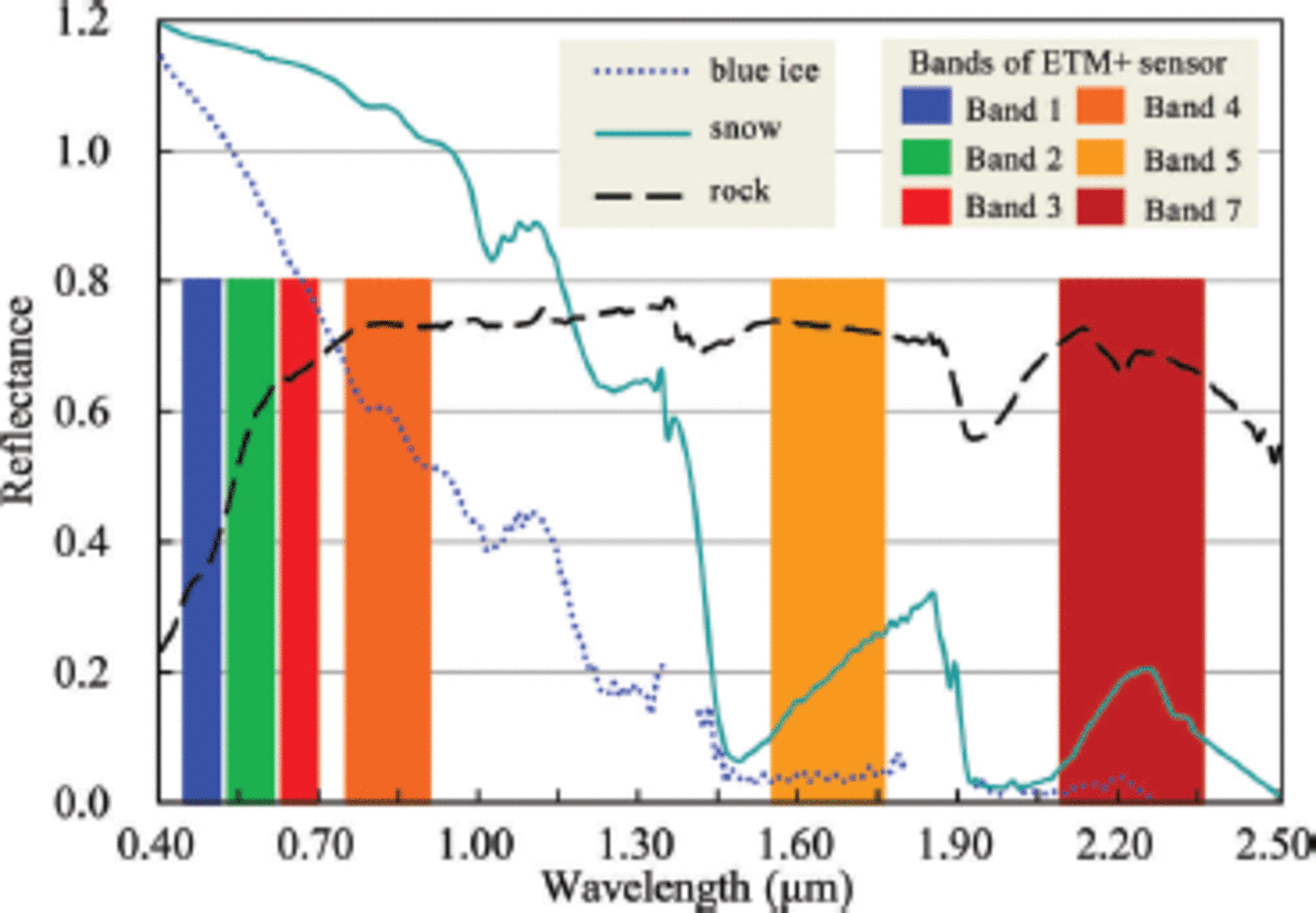
Fig. 1. Spectral reflectance of blue ice, clean snow and exposed rocks near Zhongshan station, Antarctica, in December 2009. The spectra of blue ice, snow and rocks were measured at 69 ° 27.242• S, 76 ° 21.134• E on 22 December 2009, at 69 ° 19.314• S, 76 ° 27.517• E on 12 December 2009 and at 69 ° 22.286 •S, 76 ° 22.061• E on 24 December 2009. It was sunny and breezy when the spectra measurements were taken. The six bars from left to right are the blue, green, red and near-infrared bands respectively (bands 1–4) and two SWIR bands (bands 5 and 7).
To cover the whole Antarctic continent requires a great amount of Landsat-TM/ETM+ data. In this study, 14 sample ETM+ scenes in different places were randomly chosen to define the threshold values for blue-ice identification. Previous studies indicated that BIAs, snow, rock, shadowed snow or BIAs, and shadowed exposed rock could be identified and differentiated in the Landsat TM/ETM+ images. BIAs were classified as wind-induced or melt-induced, depending on the dominant climate process, which is closely related to the mechanism of formation of the BIAs (Reference WintherWinther, 1994; Reference Liston, Bruland, Winther, Elvehøy and SandListon and others, 1999; Reference Winther, Jespersen and ListonWinther and others, 2001). They were also classified as smooth, level or rough, according to image texture information from ETM+ data. Smooth BIAs were related to wind-induced BIAs with smooth image texture, level BIAs were associated with pond and lake ice (seasonal ice) with homogeneous texture (a level, specular surface) and rough BIAs were connected with troughs, ridges and surface crevasses with a relatively rough surface (Reference Yu, Liu, Wang, Jezek and HeoYu and others, 2012). Pixels of smooth BIAs and level BIAs were almost pure, but those of rough BIAs were likely to be mixed pixels containing both blue ice and snow. In this study, training areas for different surface features were identified by visual interpretation. BIAs were only classified as smooth or rough according to pixel type (pure or mixed pixels). The former category was closely related to small grain size, while the latter was better related to larger grain size.
Six different types of surface features were used as training samples: smooth BIAs; rough BIAs; snow; exposed rock; shadowed snow or BIAs; and shadowed exposed rock. First, we selected training samples for these six types through visual interpretation of 14 randomly selected false-color composite images, which were combined by bands 7, 4 and 1. Because the 14 sample images were randomly selected, not all the six different types of surface features were included in each sample image. Next, some statistical variables – maximum, minimum, mean, standard deviation of the apparent reflectance and R 47, and the number of pixels – were calculated for all the training samples in each image. Finally, comparative analyses were carried out to determine the threshold values for BIA identification.
The mean and standard deviation of apparent reflectance of six bands for each surface feature type as derived from our training samples in 14 sample images are listed in Table 1, and the mean R 47 value of each surface feature type in each sample image as derived from our training samples is shown in Table 2.
Table 1. The mean (p) and standard deviation (SD) of apparent reflectance of six bands for each surface feature type as derived from our training samples
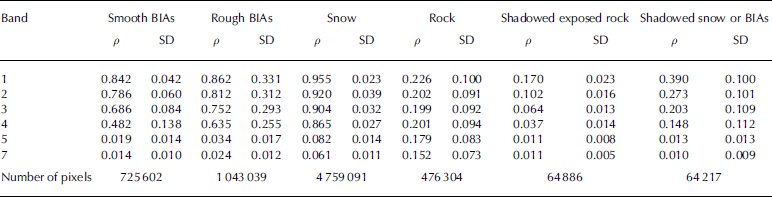
Table 2. The mean R 47 value of each surface feature type in each sample image as derived from our training samples
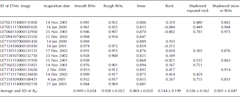
Table 1 shows that of the six types of surface, snow had the highest apparent reflectance in the VNIR wavelengths (bands 1–4) while shadowed exposed rock had the lowest; both had only slight fluctuations and small standard deviations. The apparent reflectance of smooth and rough BIAs was the next highest after snow, but the roughest BIAs had greater ranges and high standard deviations, likely caused by the mix of snow and BIAs in the pixels. The apparent reflectance of shadowed snow and BIAs was lower, but changes in the apparent reflectance from band 1 to band 4 were successively reduced, as were those of smooth BIAs, rough BIAs, snow and shadowed exposed rock. Rock showed the highest reflectance of all six types for the SWIR wavelength (bands 5 and 7). The results are consistent with those obtained from the LIMA dataset for Lambert Glacier basin (Reference Yu, Liu, Wang, Jezek and HeoYu and others, 2012).
Table 2 shows that R 47 values of smooth and rough BIAs were >0.900 (minimum value 0.901), those of snow were <0.900 (maximum value 0.894), those of rock were <0.500 and those of shadowed exposed rock and shadowed snow or BIAs were unsteady with wide fluctuations and a maximum value of 0.914; the large range is likely associated with terrain, grain size and scattered light. In Table 1, the R47 values of smooth and rough BIAs are >0.90, the highest for any area.
Tables 1 and 2 suggest that pixels with R47 values greater than 0.90 cannot be identified as blue ice because pixels containing shadowed snow or BIA pixels could be misidentified as blue ice. Previous studies showed that BIAs have a lower albedo (0.50-0.70) than snow (0.80-0.90) (Reference Bintanja and BroekeBintanja and Van den Broeke, 1994, Reference Bintanja and Van den Broeke1995; Reference Bintanja, Jonsson and KnapBintanja and others, 1997; Reference BintanjaBintanja, 1999; Reference Reijmer, Bintanja and GreuellReijmer and others, 2001; Reference Warren, Brandt, Grenfell and McKayWarren and others, 2002), so the apparent reflectance could be used as another criterion to identify BIAs. In Table 1 the reflectance of bands 3 and 4 distinguishes among the six different surface features well. Band 4 exhibits the greatest difference between itself and the other bands.
The band 4 average reflectance of smooth and rough BIAs (0.482 ±0.138 and 0.635 ±0.255, respectively) was lower than that of snow (0.865 ± 0.027) and much higher than that of shadowed snow or BIAs (0.148 ±0.112). Maximum and minimum values of reflectance of the six surface features in the 14 sample images were obtained and plotted (Fig. 2). Figure 2 clearly shows that the maximum and minimum reflectance of both smooth and rough BIAs in band 4 were lower than those of snow and much greater than those of the other three surface features. The maximum reflectance of BIAs was lower than that of snow. Pixels with band 4 reflectance between 0.30 and 0.70 could be identified as BIAs. Therefore, the criteria to identify BIAs were defined as having both R 47 > 0.900 and band 4 reflectance between 0.3 and 0.70.
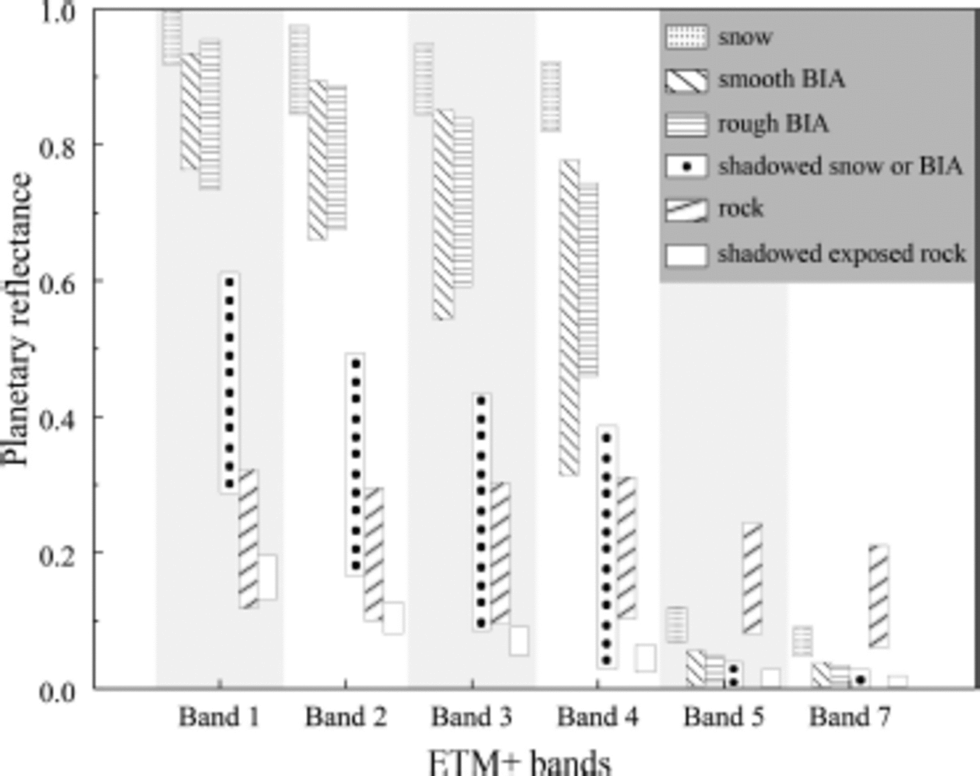
Fig. 2. Maximum and minimum reflectance values of the six surface features in the 14 sample images. In each bar the top is the maximum, and the bottom the minimum, value of apparent reflectance.
The difference in spectral characteristics between smooth and rough BIAs is clearly very small (Fig. 2). It was therefore very difficult to distinguish smooth from rough BIAs using just their spectral signatures. In this study, we focused on mapping BIAs and identifying their spatial correlation with ice velocity and elevation; we gave less attention to identifying the types of BIAs.
Threshold-based snow grain size for MOA dataset
BIAs covering the area south of 82.5° S were mapped using the SGS image of the MOA dataset. BIAs were considered when snow grain size was >400 (Reference Scambos, Haran, Fahnestock, Painter and BohlanderScambos and others, 2007).
All data were processed using a procedure developed using ENVI software (Exelis Inc., McLean, VA) and Interactive Data Language (IDL; Exelis Inc., McLean, VA, USA).
Noise reduction
BIAs were identified using R47 values and band 4 reflectance, and the resulting images were converted into binary images. To reduce this ‘salt-and-pepper’ effect and produce more realistic maps, a median filter with 5 x 5 pixel windows was applied. This filter is less sensitive than linear techniques to extreme changes in pixel values; it can remove salt-and-pepper noise and preserve useful details in images without significantly reducing the sharpness of an image. This method proved effective at removing most of the noise, though some noise still remains in the final images.
Results and Discussion
We observed a total BIA of 234 549 km2 across Antarctica, of which 29402 km2 was obtained from the SGS image of the MOA dataset covering the area south of 82.5° S, and the rest from ETM+ data covering the area north of 82.5° S. BIAs were usually located along the coast or near areas of exposed, ice-free rock. Figure 3 shows BIA distribution in Antarctica, and also in the Grove Mountains, where there were great differences between BIAs with salt-and-pepper noise obtained from ETM+ data and BIAs smoothed by a median filter with 5 x 5 pixel windows. This demonstrates the improvements achieved by the filtering process.

Fig. 3. The distribution of BIAs in (a) Antarctica and (b) the Grove Mountains. (a) The latitude of the red circle is 82.5° S, and within the circle (area south of 82.5° S) Landsat has no coverage because of its near-polar orbit. BIAs over the area south of 82.5° S were obtained from the SGS image of the MOA, and the others were obtained from ETM+ data. (b) Gray indicates BIAs filtered by a median filter with 5 x 5 pixel window size, and red indicates BIAs obtained from ETM+ data with no processing.
Accuracy assessment
It is too difficult to carry out field surveys in Antarctica to assess the accuracy of our remotely sensed BIA mapping. Instead, we use results from recently published papers as validation data. Approximately 60 000 km2 and possibly as much as 241 000 km2 of BIAs were observed in NOAA AVHRR data acquired during 1980-94 (Reference Winther, Jespersen and ListonWinther and others, 2001). That study’s maximum area of 241000 km2 is essentially consistent with our results of 234 549 km2. The Grove Mountains contained 601.9 km2 of BIAs according to ETM+ data acquired on 18 January 2001 (E and others, 2011), 610.1 km2 according to MODIS data acquired on 17 January 2001 (E and others, 2011) and 745.3 km2 according to MODIS data acquired during the 2003/04 austral summer (Reference Scambos, Haran, Fahnestock, Painter and BohlanderScambos and others, 2007). Our objective study found 624.2 m2 of BIAs in the Grove Mountains, which agrees with the results of E and others (2011) but differs by >100km2 from the MODIS summertime data of 2003/04. Reference Scambos, Haran, Fahnestock, Painter and BohlanderScambos and others (2007) reported five BIAs as blue-ice regions using the MOA dataset. Only one BIA was found in our result (69.5660 S, 43.566° E). The other four sites were not identified, for reasons discussed in the following subsection.
The differences between previous results and our results may be due to temporal changes in BIAs, the use of different identification algorithms or the different spatial and spectral resolutions of the sensors.
The size of BIAs may have changed during the past few decades and over the years between AVHRR, MODIS and ETM+ image acquisitions due to changes in wind speed, air temperature (solar radiation) and ice flow velocity, factors that could affect BIAs. The areas and spatial distributions of BIAs determined from satellite images at the same place but at different acquisition times could vary widely. Smaller areas of blue ice would become exposed when strong winds blow thin snow over BIAs, while the melting of that thin snow in periods of higher air temperatures would expose larger BIAs. The seasonal and annual changes of BIAs may be significant, so BIA changes need to be confirmed by more detailed studies.
The different spatial and spectral resolutions of the AVHRR, MODIS and ETM+ data likely also affected the differences in the various BIA calculations. Pixels containing both blue ice and snow in the 1100m resolution AVHRR data and in the 250 m resolution MODIS data (or in the 125 m gridding-space MOA data) can either be omitted or counted as BIAs, leading to either an underestimate (pixels being omitted) or an overestimate (pixels being counted) of BIAs. However, these pixels were clearly recognized in the 15 m resolution ETM+ data. Previous studies suggest that uncertainties such as mixed pixels, crevasses and shadows could account for the difference between identified BIAs (~60000km2) and the potential maximum area (241000 km2) obtained from the NOAA AVHRR data (Reference Winther, Jespersen and ListonWinther and others, 2001). Figure 1 indicates that the spectral signatures of the six-band ETM+ sensor discriminated surface features more sensitively than those of the two-band AVHRR and MODIS data, which discriminated BIAs from exposed rock and snow. The higher spatial resolution and better spectral signatures of the ETM+ data improved BIA recognition. In the future, 16-bit images with nine spectral bands from the Landsat-8 Operational Land Imager (OLI) will play an important role in mapping BIAs.
The areas and spatial distribution of BIAs obtained by different methods may have differed because of different underlying assumptions and theories. In summary, our estimates for the areas and spatial distribution of BIAs are likely to be an improvement over previous results from AVHRR and MODIS data.
Spatial distribution
BIAs identified from 1999-2003 ETM+ data covered ~1.67% of the area of Antarctica and were scattered over the continent but generally located in coastal or mountainous regions. Figure 3 shows that BIAs were concentrated in four regions: Victoria Land, the Transantarctic Mountains, Dronning Maud Land and the Lambert Glacier basin. They were sparsely distributed in other regions. These results are in agreement with previous studies (Reference Winther, Jespersen and ListonWinther and others, 2001; Reference Brown and ScambosBrown and Scambos, 2004; Reference Scambos, Haran, Fahnestock, Painter and BohlanderScambos and others, 2007; E and others, 2011; Reference Yu, Liu, Wang, Jezek and HeoYu and others, 2012). These four regions either contain nunataks or mountains with high elevations and steep slopes or are at relatively low elevation and have notable glacier dynamics. BIAs seldom occur in West Antarctica and the Antarctic Peninsula. This is generally due to higher snow accumulation and a relatively brief melt season, and the predominantly springtime acquisition time of the images used in LIMA and MOA. High snow accumulation regions require an intense melt season before the winter-spring snow accumulation is converted to surface ice. Moreover, winds are more variable, and more frequently tied to synoptic weather systems rather than highly sublimating katabatic processes. Although a late-summer acquisition and BIA analysis is possible, problems would arise in distinguishing wet snow from blue ice using the methods we present here, so in our results BIAs are less distributed in West Antarctica and the Antarctic Peninsula.
BIAs were associated with surface mass balance and ice velocity features (Reference Ligtenberg, Lenaerts, Van den Broeke and ScambosLigtenberg and others, 2013). Overlay analysis between BIAs and Antarctic ice velocity data with 450 m spatial resolution (Reference Rignot, Mouginot and ScheuchlRignot and others, 2011a, Reference Rignot, Mouginot and Scheuchlb) and digital elevation models (DEMs) with 1000 m spatial resolution (Reference Bamber, Gomez-Dans and GriggsBamber and others, 2009a, Reference Bamber, Gomez-Dans and Griggsb) was conducted (Fig. 4 and 5). Because there were great differences in map scale between the BIA data, ice velocity data and the DEM, approximately 9342 km2 and 15 122 km2 of BIAs in the overlay analysis of ice velocity data and the DEM were ignored. Statistical analysis was performed only on overlaid data between BIAs and ice velocity and DEM.
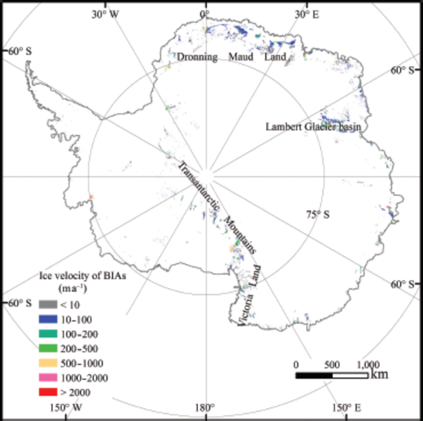
Fig. 4. BIA distribution of different classes of ice velocity.
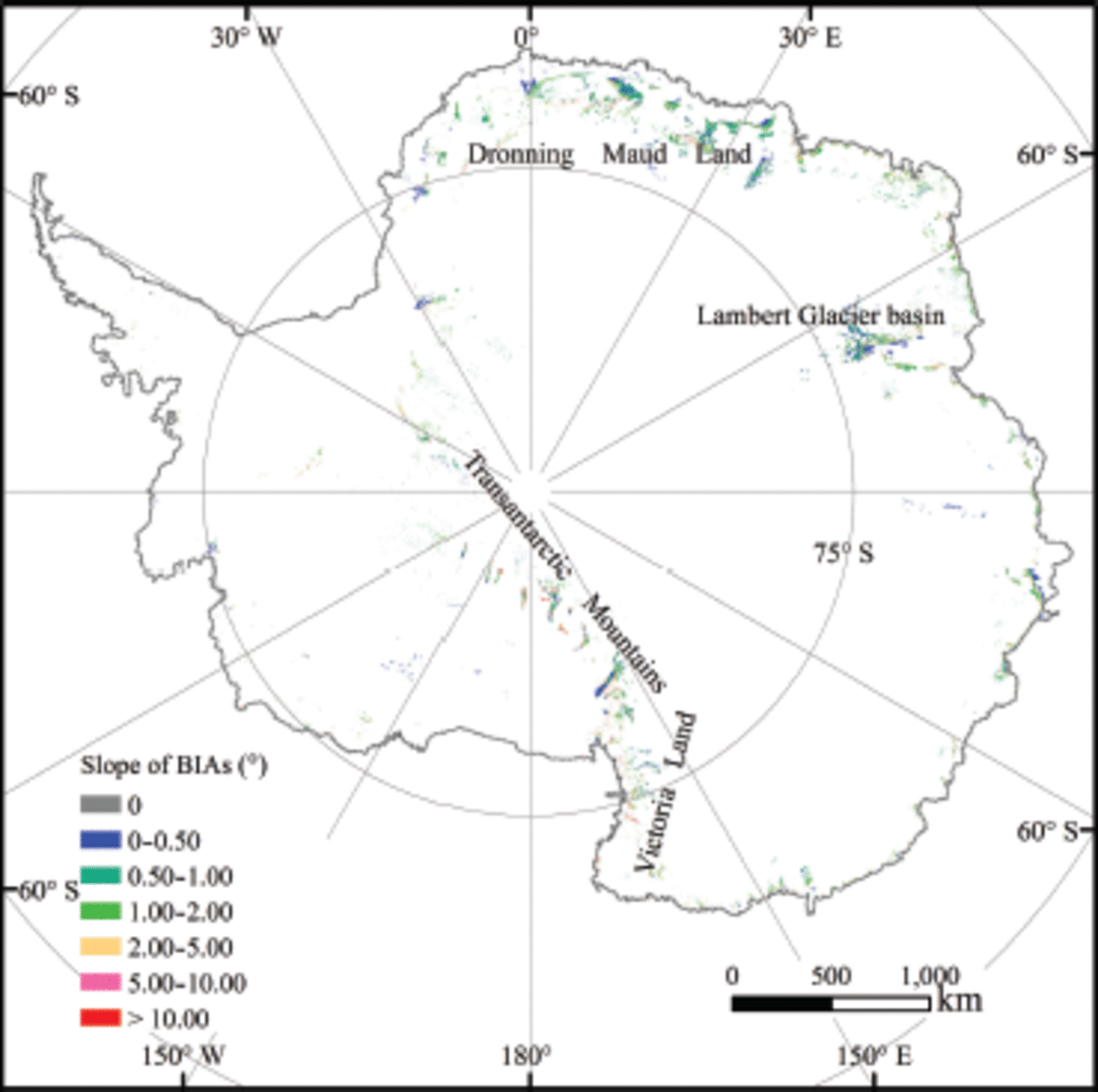
Fig. 5. BIA distribution of different classes of surface slope.
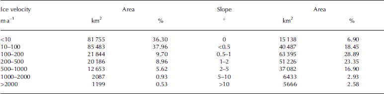
The results in Table 3 demonstrate that the ice velocity in -74.26% of BIAs was <100ma–1, and in about half these cases <1 ma–1, while 9.70% of BIAs had an ice velocity of 100-200 m a–1, 8.96% an ice velocity of 200-500 ma–1, and 5.62% an ice velocity of 500-1000ma–1. Ice velocity exceeded 1000 m a–1 for only ~1.46% of BIAs. Regions with an ice velocity of 200-500ma–1 were situated on the Ross, Shackleton, Amery, Riiser-Larsen and Ronne ice shelves, which are closely associated with glacier dynamics. The results in Table 3 show that 54.24% of BIAs had surface slopes less than 18, and 23.35% had surface slopes of 1-28. Surface slopes of only 5.51% of BIAs, at most, were >58, these areas being primarily located in the Transantarctic Mountains and Victoria Land.
Table 3. Areas and percentage of BIAs for different classes of ice velocity and surface slope
Surface slopes of BIAs with ice velocities greater than 500 m a–1 ranged from 0 to 39.058, but 96.65% of these BIAs had slopes smaller than 5° and were distributed along ice-shelf coastlines. This suggests that BIAs with higher ice velocities may occur on flatter glaciers with smaller surface slopes. BIAs with surface slopes greater than 5° had ice velocities between 0 and 2832 m a–1, but the ice velocities of 95.27% of these BIAs were <500ma–1. However, BIAs with slopes greater than 5° and ice velocities greater than 500 m were dispersed across Antarctica. BIAs with gentle slopes but greater ice velocity were mainly distributed on coastal ice shelves, and inland BIAs with steeper slopes but slower ice velocity were mainly distributed along or near mountains. This suggests that there was no significant relationship between ice velocity and surface slope; the relationship may be evident when rough and smooth BIAs are separated.
The spatial resolution of the Antarctic ice velocity map and DEM (900 m and 1000 m, respectively) was much coarser than that of the BIA map (15 m): at least 60 x 60 pixels in the ETM+ data constitute only one pixel in the Antarctic ice velocity map and DEM. As a result, the ice velocity and surface slope of the BIAs could not be described at high resolution. Errors may have resulted from this large difference in spatial resolution among the datasets. The dates of data acquisition also varied greatly: ETM+ data were acquired from 1999 to 2003, ice velocity data were created from SAR data acquired from 2007 to 2009, and the DEM was generated using Satellite Radar Altimeter (SRA) data from European Remote-sensing Satellite- 1 (ERS-1) acquired from 1994 to 1995, and Geosciences Laser Altimeter System (GLAS) data from the Ice, Cloud and land Elevation Satellite (ICESat) acquired from 2003 to 2008. Temporal changes could also lead to inconsistent spatial alignments of BIA locations, ice velocities and the DEM, which could also lead to errors.
Conclusions
In this study, BIAs in Antarctica have been mapped from 15 m spatial resolution Landsat-7 ETM+ images and the 125 m grid-spacing snow grain-size image of the MOA using thresholds based on band ratio and reflectance. The geographical distribution of BIAs was delineated and compared with spatial patterns in ice velocity data and surface slopes provided by DEMs. The results estimated that BIAs occupy 234 549 km2, or 1.67% of the continent. BIAs were scattered widely over the continent but were generally located in Victoria Land, the Transantarctic Mountains, Dronning Maud Land and the Lambert Glacier basin. The results were reasonable, realistic, and consistent with previous studies, although they differed from previous results because of possible temporal changes, different algorithms and different spatial and spectral resolutions of the sensors. The results of overlay analysis indicated that the ice velocities of ~92.92% of the BIAs were <500 m a–1, while 74.26% of BIAs exhibited ice velocity of <100 m a–1. The surface slope of most BIAs was <50, and 54.24% of BIAs had slopes of <1 8.
We have focused on generating a BIA dataset with high spatial resolution. This dataset will be useful for many applications, including surface mass- and energy-balance models, meteorite searches, paleoclimate studies and airstrip site selection. It can also serve as a base dataset for identifying future changes to BIAs. People will download this dataset from NSIDC soon. Temporal changes, including seasonal and annual changes, of BIAs may be significant; they may be caused by short-term snow accumulation, strong winds or other meteorological and environmental conditions. Refined results will be obtained using SAR data and new optical-sensor data (e.g. OLI data). Detailed BIA classification for applications should also be conducted in the future.
Acknowledgements
This work was supported by the Chinese Arctic and Antarctic Administration, the National Natural Science Foundation of China (grant No. 41106157), the National Basic Research Program of China (grant No. 2012CB957704), the National Natural Science Foundation of China (grant No. 41176163), the Fundamental Research Funds for the Central Universities, Chinese Polar Environment Comprehensive Investigation and Assessment Program, and the Special Foundation for Young Scientists of State Key Laboratory of Remote Sensing Science (grant No. RC12-7). Support was also provided by NASA grant NNX10AL42G. We are grateful to NSIDC for providing the snow grain-size image of the MODIS-based MOA dataset, ice velocity data and DEM data, and for hosting this dataset and creating a web page for it. Two anonymous reviewers are thanked for their comments.


