Introduction
It is difficult to observe and obtain measurements of water flow within and beneath glaciers. Thus, studies of the fluctuation and chemical characteristics of glacial stream water significantly contribute to the understanding of subglacial flow processes. For example, Reference CollinsCollins (1979) examined the variation of solute concentration and water discharge in two neighboring glaciers. He concluded that subglacial and englacial flow paths existed and inferred that the subglacial hydraulic processes were different in the two glaciers. In another study, Reference Humphrey, Raymond and HarrisonHumphrey and others (1986) correlated pulses of high sediment concentration with mini-surge events, from which they estimated the velocity of subglacial water, and concluded that the subglacial hydraulic system was composed of many small passageways. Given that these relatively simple stream measurements provide the basis for significant insights into subglacial processes, they were included in a study at South Cascade Glacier.
During the summers of 1986 and 1987, a field study investigated the hydraulics of subglacial water movement at South Cascade Glacier. The study included measurements of water discharge, electrical conductivity and suspended sediment in streams flowing from the glacier to determine the source regions of the water and provide the basis for a conceptual model of how water is routed through the glacier. Other measurements included water levels in boreholes drilled to the glacier bed, to define the pressure of the subglacial system, and tracer injections to determine the flow speed and dispersion of the system. The results and analysis of the stream-flow data arc given in this paper, whereas the discussion of borehole and tracer studies will be presented in subsequent articles.
Site Description and Study Methods
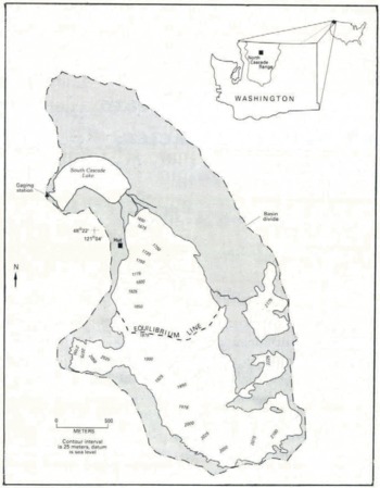
South Cascade Glacier is a small, temperate glacier located along the crest of the North Cascade Range in Washington State, U.S.A. (Fig. 1). The glacier is about 3.4 km long, 2.6 km2 in area and is situated within a hydrologically well-defined drainage basin with an area of about 6.1 km2. The elevation of South Cascade Glacier ranges from about 1620 to 2200 m. The climate at the glacier is maritime with an average annual temperature of +1°C (Reference Meier, Tangborn, Mayo and PostMeier and others, 1971). Most precipitation falls in the winter as snow, which has a mean water equivalent that usually exceeds 2.5 m. The large winter snow accumulation and warm summer temperatures produce an active glacial hydrologie system in the glacier.

Fig. 1. South Cascade Glacier basin and adjacent ice patches based on aerial photography taken on 24 September 1985. The. position of the equilibrium line is the approximate ancrage location.
Four streams, denoted by numbers (1–4), drain the terminus region of South Cascade Glacier (Fig. 2). In the summer of 1986, the four streams maintained separate channels. Stream 1 drained the margin on the cast side of the glacier and stream 2 drained a proglacial pond, the source of which was a submerged ice tunnel. Stream 3, which had the greatest discharge, flowed from an ice tunnel at the center of the terminus and stream 4 drained the western margin of the glacier. By the summer of 1987, the glacier had retreated approximately 3 m at the center of the terminus, and the courses of streams 3 and 4 had changed. Stream 3 drained into the proglacial pond and stream 4 flowed under the glacier margin and could not be monitored.

Fig. 2. Location of the gaging stations
During each field season, the discharge of each stream was calculated about once a week using paired depth and velocity measurements at 10–20 uniformly spaced locations across each channel cross-section. The resulting stage discharge relation was used to convert the recorded stage measurements to discharge values. Severe rainstorms changed the stage–discharge relation several times during the field season. Two sources of uncertainty in the discharge estimates are turbulence in some streams that disturbed velocity measurements and porous gravel channels in others that allowed a significant proportion of the water to move by percolation (personal communication from J.D. Smith, University of Washington, 1987). A conservative estimate of the error in the discharge values is 10%.
The electrical conductivity of each stream was measured using a dip cell fixed to a weighted post residing on the stream bottom. The probes were calibrated several times during the field season using solutions of known electrical conductivity cooled to the temperature of the stream water. The electrical conductivity of water is a measure of the ion concentration of dissolved solids (Reference HemHem, 1989). If the relative proportion of individual ion species does not change, a linear relation exists between the electrical conductivity and the mass of charged dissolved solids. Electrical conductivity measurements were converted to cation concentration using the data of Reference Reynolds and JohnsonReynolds and Johnson (1972), who studied the chemistry of surface waters in South Cascade basin. No conversion to total mass of dissolved solids was attempted because of the presence of a substantial amount of silica, which has no charge, and therefore cannot be detected by electrical conductivity. A high correlation (r = 0.99) was found for a linear relation between electrical conductivity and cation concentration (cation concentration in gm−3 = 0.2(electrical conductivity in µS) – 0.002). Anions were not included in the relation because chloride, a major species, was frequently inferred rather than measured (Reference Reynolds and JohnsonReynolds and Johnson, 1972). Because concentrations of cations and anions are approximately equal, the cation concentration can be considered a good indicator of total charged ion concentration. The cation load (gs−1) was calculated from multiplying water discharge by cation concentration.
The light transmittance of water (turbidity) can be used to estimate the concentration of suspended sediment in otherwise transparent water (Reference Humphrey, Raymond and HarrisonHumphrey and others, 1980). An instrument to measure turbidity was constructed using a light-emitting diode and sensor with a voltage output. The instrument was calibrated by collecting grab samples of stream water during a turbidity measurement, filtering the sample and weighing the residue of sediment. The relation between the mass of suspended sediment and voltage output of the instrument was linear, over the concentration range measured, with a correlation coefficient of 0.94.
The meteorological measurements in both field seasons included precipitation, air temperature, humidity and solar radiation. All stream-flow and meteorological data were recorded by digital, solid-state data loggers at time intervals no longer than 1 h. The turbidity was recorded hourly on an analog recorder.
Meltwater reharge to the glacier was estimated from weekly measurements of surface lowering at stakes drilled into the ice and firn at the beginning of the ablation season. Daily recharge of meltwatcr was interpolated from the weekly measurements by using a multiple linear regression with independent variables of mean daily air temperature and Julian day (an index of solar angle). The relation was re-scaled for each interval between measurements using the total lowering for that interval. The daily specific water input was calculated by adding the mean daily meltwater input to measured daily rainfall.
Comparison of Stream Measurements
Stream 1 differs from the other streams measured at South Cascade Glacier. This stream drains talus slopes on the east side of the basin and is similar to a spring; the discharge is nearly constant with almost no diurnal variation. Two exceptions occurred in mid-July 1987, when storms caused the glacier margin near stream 1 to flood and partially drain into the stream. The cation concentration is large compared to that in other streams (Table 1), indicating that the water has been in contact with rock for a longer time than has water in the other streams. The 198G values were not included because they were affected by algal growth on the probe.
Table 1. Summary of the stream measurements at South Cascade Glacier. M is the mean, SD is the standard deviation, Cv s the coefficient of variation, which is the standard deviation divded by the mean and is a normalized measure of variation, and – indicates no data

Streams 2 and 3 are typical of streams sustained by glacier meltwater; these streams have significant diurnal fluctuations in discharge and cation concentration (Figs 3 and Figs 3 and 4). The water discharge of stream 3 is approximately twice that of stream 2 and the discharge for both streams was greater in 1986 than in 1987 (Table 1). The latter difference was caused by a number of factors, including precipitation and errors in discharge measurements that overestimated the discharge in 1980. The larger variation in diurnal discharge in 1987 compared to that in 1986 probably resulted from earlier exposure of bare ice.

Fig. 3. Results of measurements made in stream. 2 for the 1986 and 1987 field seasons.

Fig. 4. Results of measurements made in stream 3 for the. 1986 and 1987 field seasons.
The cation concentrations of streams 2 and 3 are similar and show diurnal variations. Stream 3 had a larger mean concentration in 1987 than in 1986 (Table 1) because the stream record extended into September during a period of greater concentration. The variation in concentration was also larger in 1987 than in 1986, resulting from the increased discharge variation. For both streams, the cation concentration varies inversely with discharge.
Stream 3 appeared visually to have the greatest concentration of suspended sediment of all the proglacial streams. Thus the turbidity probe was set in stream 3 during midsummer of 1987. The suspended-sediment data (Fig. 4) indicate a marked diurnal variation as well as long periods of substantial variability.
Surface Hydrology
Delay of Daily Peak Discharge
The discharge hydrographs for streams 2 and 3 indicate that the time of daily peak discharge changes during the season. Figure 5 shows that for 1987 the peak discharge occurred at roughly 2200 h PDT in early July, but by mid-August it appears at roughly 1600 h PDT and thereafter was constant.

Fig. 5. Time of daily peak water discharge (open circles) for streams 2 and 3 during the measurement period in 1987. The dashed line is the interpolated snowpack thickness at the equilibrium line; open diamonds indicate measured thickness; and the solid circles are times of daily peak discharge following a snowfall.
The processes of water flow through snow can explain the decreasing delay in daily peak discharge. Figure 5 shows the correlation between the time of daily peak discharge and snow depth at the equilibrium line. This correlation is a result of the transit time of the water wave through snow and depends on the wave speed through the unsaturated zone along the vertical path and in the saturated flow at the base. Experiments on water flow through snow at South Cascade Glacier (Reference Colbeck and DavidsonColbeck and Davidson, 1973) indicate that the speed of the peak meltwater wave in unsaturated snow is about 0.3 m h−1. In early July 1987, the snowpack thinned to about 2 m at the equilibrium line and to zero near the terminus. Using an average snowpack thickness of about 1 m, the transit time of the peak meltwater wave passing through the vertical dimension would be about 3 h, half the 6 h delay in the time of daily peak discharge observed for streams 2 and 3.
Once the water reaches the impermeable ice surface underneath the snow it begins to move along the ice surface in a saturated layer. The transit time, t, of the water can be estimated (Reference ColbeckColbeck, 1974) from:
where u is the effective porosity of the snow, L is the length of the flow path along the snow–ice interface, a is equal to the water density times gravity divided by water viscosity, Ks is the permeability of the saturated snowpack and S is the slope of the snowpack. Using approximate values of 0.45 for u, 10−10 m2 for K s and 0.2 for S yields t = 1.14L, where t is now in hours. To explain a 3 h delay, L would have to be about 2.6 m, a reasonable separation between crevasses in many parts of the ablation zone of South Cascade Glacier.
Further evidence for delay caused by the slow movement of water through the saturated base of the snow is provided by the effects of a late summer snowfall. Prior to 14 September 1987, the ablation zone was completely clear of snow. A snowfall on the evening of 14 September 1987 blanketed the glacier with about 25 cm of snow. By 18 September, the snow was 16 cm thick and the time of the peak discharge in stream 3 was delayed by about 3.75 h from pre-storm values (Fig. 5). Two days later, on 20 September, the time of daily peak discharge was back to normal, which coincided with the disappearance of the new snow from the ablation zone of the glacier. The estimated transit time of the meltwater wave through the snowpack on 18 September is 0.5 h, which together with a 3 h travel time along the snow–ice interface gives a total delay of 3.5 h, which is close to the actual delay of 3.75 h.
It is unlikely that enlarging conduits is reponsible for the changing delay in peak flow as suggested by Reference EllistonElliston (1973). This can be shown by examining the hydraulics of conduit flow, assuming that conduits are primarily responsible for englacial and subglacial water transport. If the conduit is flowing full, then any change in water discharge (caused by input variations) will affect conduit pressure. The resulting pressure wave is transmitted almost instantaneously to the terminus. The speed of the pressure wave is related to the compressibility of the water, tunnel walls and air content in the water (Reference Wylie and StreeterWylie and Streeter, 1983). Therefore, peak discharge should occur only moments after peak input. If the water is flowing in a partly full conduit, then the appearance of peak flow in the outlet streams is related to the time required for a monoclinal wave to propagate to the terminus. The kinematic approximation for the wave speed is a function of the ratio of the changing discharge to the changing cross-sectional area, c = dQ/dΑ, known as the Kleist–Seddon formula (Reference WhithamWhitham, 1974, p. 81). In a circular cross-section, the wave speed is greater than the flow speed until the water reaches 83% of the diameter, then the flow speed exceeds the wave speed. The reversal is a result of the frictional term of the momentum equation increasing faster than the pressure gradient. In this region, an instability is present because full pipe flow can flow faster, for the same discharge, than if the flow depth is equal to, or greater than, 83% of the flow depth. A small perturbation, such as a wave, can change the flow conditions from partly full to full conditions.
At the onset of surface melt in the spring, the subglacial conduits are at their smallest radius because of ice closure during the winter (Reference RöthlisbergerRöthlisbergcr, 1972). Most likely, the conduits would be flowing full at this time and the effect of any change in melt input would quickly be transmitted to the stream terminus. As the season progresses, the conduits enlarge and the flow would tend to be open channel. Thus the response to a change in surface input would be slower, and one would expect the time delay to increase during late summer. However, the change in travel time for a monoclinal wave in open-channel flow of different cross-sectional areas is small relative to the large delays (about G h) caused by flow through the snowpack. Therefore, an “enlarging” system would have little effect on the response time of the terminus stream to daily fluctuations in meltwater input.
Reference EllistonElliston (1973) demonstrated that the daily variation of direct run-off became more peaked as the season progressed. This also can be explained by water flow through snow. Saturated flow through a porous medium, such as snow, dampens the diurnal input variation compared to overland or channelized flow. As the snow line retreats up-glacier, more ice surface is exposed and more surface meltwatcr moves as overland flow rather than by percolating slowly through the snowpack. The effect on the hydrograph is a steeper rising limb and, because water storage on the ice surface is negligible, the falling limb of the hydrograph also steepens. Thus, as the season progresses and the snow line retreats, the hydrograph becomes more peaked.
Evidence for Multiple Water-Drainage Basins in the Glacier
When multiple streams flow from a glacier, it is reasonable to question whether the glacier contains water-drainage divides. To delineate the drainage divides for each stream flowing from the glacier, tracers were injected into crevasses, boreholes and marginal streams flowing into the glacier. Results of seven injections made in 1986 allowed a rough delineation of water divides. The positions of these divides were refined and extended in 1987 when 37 more injections were made.
The tracer injections define drainage divides on the lower part of the glacier, but the positions of the divides on the upper part and along the valley walls arc conjectural. To refine better the positions of the drainage divides, a water balance, based on a comparison between estimated water recharge (rain and icemelt) and measured stream discharge, was calculated for each basin. The water balance for each basin can be expressed as

where A is the area of the drainage basin, q is the time-dependent water input per unit area, Q is the measured stream discharge that drains the basin, M is the specific storage of water, a time-dependent quantity expressed as volume per unit area per unit time, and t defines the time period of measurement. The subscript i refers to the basin. The specific storage is assumed to be the same for each basin.

The quantities in Equation 2 were integrated over the period of the whole field season to avoid errors in daily melt estimates and short-term changes in water storage in the glacier. The positions of the drainage divides were adjusted so the area of each basin matched the area calculated by Equation 2. The positioning of the extrapolated boundary was subjective and determined, in large part, by surface topography.
The locations of the drainage divides are presented in Figure 6 and results of the calculations are summarized in Table 2. No tracer appeared in stream 1, indicating that this stream drains only the talus slopes on the east side of the ablation zone. Stream 2 drains the eastern half of the ablation zone and adjacent eastern slopes. Stream 3 drains the accumulation zone and adjacent slopes, and most of the western half of the ablation zone. The existence of a narrow drainage strip through the lower ablation zone suggests that the flow from up-glacier becomes concentrated and probably flows through a single conduit within the strip. Finally, stream 4 drains a small area along the glacier’s western margin and adjacent slopes.

Fig. 6. Location of tracer injections and of glacier-drainage basin divides.
Table 2. Summary of the estimated water input, output and storage values for South Cascade Glacier

The 1987 values in Table 2 are more reliable than those in 1980 because more ablation stakes were set and were read more frequently during 1987, thus reducing errors in space and time. However, the estimated fraction of glacier area for each basin differs by only 2% when the values for 1985 and 1987 are compared. In 1987, the storage change in each basin, during the measurement period, was −13% of the volume of stream flow and indicates a net loss of water from storage in agreement with Reference Tangborn, Krimmel and MeierTangborn and others (1975). However, considering the unknown but sizeable errors involved in estimating the snowmelt and precipitation, as well as the errors in the discharge measurements, a −13% difference can be explained by the errors alone without a storage mechanism.
The positions of surface-drainage divides differ from those of subglacial divides as illustrated by the results of paired tracer injection, one at the bottom of a borehole and the other in a nearby surface crevasse (labeled A in Figure 6). The tracer injected at the surface appeared in stream 2 whereas the tracer injected at the base of the borehole appeared in stream 3. The fact that surface run-off drains into a basin different from subglacial flow directly beneath indicates that the water must flow englacially for significant distances before reaching the bed.
Surface-water divides have been delineated on other glaciers such as Mikkaglaciären and Storglaciären (Reference StenborgStenborg, 1973) and Pasterzcnglctschcr (Reference BurkimsherBurkimsher, 1983). The year-to-year persistence of water divides, similar to those identified at South Cascade Glacier, has also been documented (Reference StenborgStenborg, 1973). However, the locations of subglacial divides are known to change as shown by tracer tests (Reference BurkimsherBurkimsher, 1983) and by data from subglacial water intakes (Reference Hooke, Wold and HagenHooke and others, 1985).
One feature unique to South Cascade Glacier is the narrow zone of drainage in the ablation zone. Like South Cascade Glacier, Storglaciären also has a subglacial ridge that forms part of the down-glacier perimeter of a closed basin (Reference BjörnssonBjörnsson, 1981), yet tracer studies have not demonstrated a similar narrow corridor, although a sub-surface corridor may not be ruled out (personal communication from R. Hooke, 1991). Two possible explanations are suggested. First, below the ridge at Storglaciären another closed basin exists that may not be conducive to flow through a single conduit. Secondly, the crevasses in the corridor of South Cascade Glacier are parallel to the path of the subglacial conduit, so that it may be the fortuitous alignment of the crevasses and conduit that permits the detection of the conduit by surface injection of tracers.
Subglacial Hydrology
One of the fundamental time-scales of water flow in glaciers is the diurnal because daily melting of snow and ice is the primary water source. Analysis of water flow and solute content at this time-scale should reveal information about the character of the hydraulic system.
Daily Stream-Flow Variations
To examine diurnal water-flow processes, an average daily hydrograph is calculated from the discharge time series by summing the discharge measured at the same time each day and dividing it by the number of days, resulting in a mean discharge for that time of day (Reference Humphrey, Raymond and HarrisonHumphrey and others, 1986). For clarity, this is mathematically expressed as

where Q t is the mean discharge at time, t; subscript d is the day and Ν is the total number of days. This procedure, henceforth called stacking, enhances the diurnal variations at the expense of variations occurring at other time-scales.
In stacking the discharge data from South Cascade Glacier, the data prior to mid-August and days with rain-fall were eliminated to remove the effects of the changing time of peak daily flow and of peaks generated by rain-fall. The results arc shown in Figure 7.

Fig. 7. Stacked time series of measured stream-flow variables for periods from 23 August to 10 September 1986 (plus symbols) and from 25 August to 30 September 1987 (dashed lines).
Generally, the water discharge rises rapidly in mid-morning after the onset of surface melt, reaching a peak in late afternoon, and then slowly decreases to a minimum by early morning of the next day. The larger discharge variation in 1987 compared to 1986 in stream 3 is caused by the earlier disappearance of snow cover on the ablation zone. The cation concentration varies inversely with discharge, reaching its maximum in mid-morning. The inverse phasing lags the discharge by ![]() during both field seasons. The cation load, however, shows a different variation between streams. Stream 3 has a slight diurnal variation but the phasing is inconsistent between 1986 and 1987 in that the load seems phased with concentration in 1986 but not in 1987. In contrast, the load for stream 2 is roughly phased with water discharge although peak load precedes peak discharge. The diurnal variation of suspended-sediment concentration in stream 3 (not shown) lags water discharge by about 1 h, whereas sediment load is in phase with water discharge.
during both field seasons. The cation load, however, shows a different variation between streams. Stream 3 has a slight diurnal variation but the phasing is inconsistent between 1986 and 1987 in that the load seems phased with concentration in 1986 but not in 1987. In contrast, the load for stream 2 is roughly phased with water discharge although peak load precedes peak discharge. The diurnal variation of suspended-sediment concentration in stream 3 (not shown) lags water discharge by about 1 h, whereas sediment load is in phase with water discharge.
The diurnal variation of stream-flow data has been examined at Chamberlain Glacier, Alaska (Reference Rainwater and GuyRainwater and Guy, 1961), for dissolved ions and suspended sediment, at Gornerglctscher, Switzerland (Reference CollinsCollins, 1978, Reference Collins1979), for conductivity, and at Variegated Glacier (Reference Humphrey, Raymond and HarrisonHumphrey and others, 1986) for conductivity and suspended sediment. In these cases the conductivity and suspended-sediment variations preceded the discharge variations, in contrast to the results from South Cascade Glacier. Differences in phasing between suspended-sediment transport and discharge variation are documented for rivers (Reference WilliamsWilliams, 1989), and therefore such a difference is not unique to glacial streams.
Two mechanisms may explain the lag observed at South Cascade Glacier: (1) a monoclinal wave, like the rising limb of diurnal discharge, propagates at a speed faster than the flow speed of the water, as previously discussed. Because the cation or sediment concentration is carried along at the water speed, rather than at the wave speed, the concentration would lag behind discharge; (2) the presence of pools along the flow path quickly transmits an increase in flow but the solutes or sediment would mix in the pool and delay their passage. The residence time of water in an instantaneously mixed pool is the pool volume divided by the water discharge. If many pools exist in a subglacial channel, the arrival time of peak concentration would significantly lag peak discharge.
Mixing Models
Some insight into the relation between water discharge, solute concentration and solute load can be provided by examining simple mixing models. The cation concentration is the ratio of the load to the discharge, C = L/Q. When the load is constant and discharge varies, the concentration changes due to dilution indicating that the sources for the water and cations are different (Fig. 8a). If the load also varies with time, the resulting concentration varies according to the ratio of the load to the discharge. The concentration varies inversely with discharge when the amplitude of the load variation is smaller than the amplitude of the discharge irrespective of their phasing (Fig. 8b and c). When the amplitudes are the same and in phase, the concentration is constant (Fig. 8d). Only when the load amplitude exceeds the discharge amplitude (Fig. 8e) docs the concentration vary with the discharge. Physical examples of solute sources include ground water, marginal streams flowing into the glacier or water flowing from a subglacial layer and dissolution of ions.

Fig. 8. Simple mixing models for water discharge, Q (solid line); solute concentration, C (dashed line); and solute load, L (dotted line). The values shown are scaled by the mean of each variable
To model the latter process, the dissolution of solute from the bedrock into the water is assumed to be a first-order rate reaction,

with the solution,
where k is a rate constant and Cmax is the maximum possible solute concentration in the water. The flow of water is approximated by the Mannings equation, Q = (AR 2/3 S 1/2)/n, a kinematic approximation, where A is the cross-sectional area of flow, R is the hydraulic radius, S is the slope and n is a roughness coefficient (Reference Roberson and CroweRobertson and Crowe, 1985, p. 388). The conduit was considered to be a half circle resting on a flat bed with radius of 1 m and approximately 1 km long. The discharge was varied from 0.75 to 1.25 m3 s−1 in a 24 h period and the flow was assumed to be uniform. Water entered the conduit with a conductivity of 1 µS and the resulting concentration was a function of its travel time down the conduit, as calculated by Equation 4. The result (Fig. 8f) is a solute load in phase with discharge and a concentration inversely phased. Although surface meltwater dilutes the solute-concentrated water at the bed, the dissolution kinetics described by Equations (3) and (4) indicate a faster dissolution for more dilute water. Whether the load varies directly with discharge or inversely denends to some decree on the magnitude of the rate constant. The case presented here is used merely to illustrate the possibility for significant dissolution.
The mixing models show that cation concentration is not a useful indicator of subglacial processes because of the effect of dilution. Rather, the load and discharge are the significant variables.
Application of the Mixing Models
Reference Humphrey, Raymond and HarrisonHumphrey and others (1986) reported a relatively constant solute load, and hence a solute concentration inversely correlated with water discharge (Fig. 8a), in a stream draining the main body of Variegated Glacier. Based on analysis of the stream discharge and estimated velocity of turbidity peaks, they concluded that the subglacial hydraulic system was composed of two regions. One region was characterized by a distributed flow system and was located, for the most part, under the accumulation zone of the glacier (personal communication from CF. Raymond, 1991). The other region, in the ablation zone, was drained by a subglacial conduit. Between the two regions a transitional zone exists that couples the two systems. The constant solute load implies a source area that is not affected by diurnal fluctuations in water discharge, and one possible source region would be the distributed flow system inferred to exist under the accumulation zone. They also noted a slight decrease in load with increasing discharge, corresponding to Figure 8b, and concluded that a small ground-water flow to the subglacial system may be responding to the variations in subglacial pressures.
Reference CollinsCollins (1979) compared stream discharge and conductivity measurements from Gornerglctschcr and neighboring Findelengletscher. To compare his results to the analysis in this paper, one has to recognize that his estimates of subglacial water flux are proportional to solute load. Therefore, the variations in subglacial water flux will henceforth be called load. The data from Gornergletscher indicate that load and concentration vary inversely with discharge, a condition corresponding to Figure 8b of the mixing models. Collins explained that the water pressure in the subglacial conduit exceeded local pressures and water was driven from the conduit to marginal storage areas. Solutes were acquired by the water during residence in these storage areas. When the influx of daily meltwatcr decreased, the pressure gradient reversed and the water flowed back to the conduit with an increased solute load. Data from Findelengletscher showed the load was phased with the stream discharge while the concentration was out of phase corresponding to Figure 8c or f. This was interpreted as indicating a subglacial system of cavities in which the slow-moving water acquired solutes. Reference Ikon and BindschadlerIken and Bindschadlcr (1986) extended this idea to a dynamically linked cavity system similar to that described in detail by Reference KambKamb (1987).
Using the mixing models and the descriptions of subglacial hydraulic systems beneath other glaciers together with the data recorded from the streams draining South Cascade Glacier, the hydraulics under each stream basin can be outlined in general terms.
The diurnal variation of the cation concentration in stream 3 can be explained in terms of a simple dilution system (Fig. 8a). The cation concentration varies inversely with the water discharge and the load is relatively constant which implies a relatively constant source. Marginal streams are not significant sources of cations because none had a cation concentration much above that for snowmelt. A subglacial source must be responsible.
The source area may be under the accumulation zone, where water input from the firn layers is more or less constant, and under the upper ablation zone, provided that the hydraulic coupling to the surface is weak, as suggested by the paired surficial and basal tracer injections. If the subglacial water is flowing in a distributed system, then flow speed is slow permitting significant dissolution to occur. At some point this distributed system must connect to the conduit flowing in the narrow drainage zone. The diurnal flux of water is supplied by surface melt in the ablation zone that reaches the subglacial conduit, at the head of the narrow drainage zone, and dilutes the less variable and solute-concentrated flow from the distributed system.
A different and informative view of the relation between cation content and water discharge is obtained by plotting the first as a function of the second. This eliminates the complexity of time and offers an unobstructed view of all the data that are otherwise eliminated by stacking.
The relation between cation concentration and water discharge in stream 3 (Fig. 9d) shows they are inversely correlated in an asymptotic manner. The maximum concentration reaches values typical of stream 1 (Table 1) and minimum concentrations arc typical of icemelt, which suggests that ground water and snowmelt define the range of concentration, and dilution is the primary process governing concentration. The cation load (Fig. 9c) is independent of discharge.

Fig. 9. Cation concentration and load as a function of water discharge for stream 2 in 1986 and stream 3 in 1987. Note the difference in scale between the figures for streams 2 and 3.
The primary feature of stream 2 is the close phasing between load and water discharge, much like the mixing model in Figure 8c or f. A marginal stream flows into the glacier near the head of this basin (Fig. 6) and may cause some of the variation in load. The flow was visually estimated at 0.012 m3 s−1, or about 10% of the flow of stream 2 at the same time, and the cation-concentration measurement was 4.0 gm−3, yielding a load of approximately 0.05 g s−1. This marginal stream is thought to be the origin of the main conduit in this basin. It is assumed that the variation in water discharge is diurnal because the source of the stream is the isolated snow and ice patches on the east valley wall of the basin. This marginal stream supplies almost one-quarter of the observed variation in load of stream 2. The remainder of the solute load must come from subglacial sources. Significant dissolution along the main conduit path is unlikely because a similar load variation is not observed in stream 3, despite the same geological environment and similar conduit length and slope. Percolation through a subgiacial debris layer may supply the observed load if the layer is sufficiently permeable to transmit diurnal variations in surface input.
The relation between cation concentration and discharge in stream 2 shows an inverse correlation (Fig. 9b), indicating that dilution again governs the concentration. But, in striking contrast to stream 3, the cation load increases with discharge until 0.7 m3s−1 is reached and thereafter remains virtually constant (Fig. 9a). The change in relation between load and discharge may be explained by filling a debris layer with water until it becomes saturated, at which time excess water flows on the surface of the debris at the ice–debris interface. This surface water would not acquire ions at the same rate as water that is percolating through the debris and consequently the cation load would no longer increase.
Model of Subglacial Flow in the Stream 2 Basin
Field observations suggest that a subglacial debris layer exists in the stream 2 basin. Whether this layer transmits most of the water was examined by modeling the flow of water through it. The problem is to calculate the pressure and flow through a thin, confined aquifer with vertical infiltration from crevasses and moulins as a distributed source. A one-dimensional pressure distribution in a confined layer may be written (Reference Freeze and CherryFreeze and Cherry, 1979) as

where h is the water-pressure head in terms of water height; Τ is the transmissivity of the layer and is equal to hydraulic conductivity times the layer thickness; S is the storativity (dimensionless) and equal to the specific storativity times layer thickness; and I is the distributed input of water expressed in m3 m−2s−1. The distributed input I is the difference between the surface-melt rate entering the glacier and the change in storage of passages (crevasses, moulins and tubes) that connect the surface to the bed. Further,

where q s is the surface-melt rate expressed as m3 m−2 s−1 and Β is the void area in the ice per unit area of the glacier’s bed. Combining Equations (5) and (6),

Equation 7 was solved numerically with a no-flow boundary at one end and a zero pressure boundary at the other. The subglacial water divide between basins 2 and 3 is considered the no-flow boundary and the conduit is considered to be usually flowing at atmospheric pressure. The initial condition was zero pressure and the model was run with a steady diurnal variation in input until a steady diurnal variation in outflow was achieved. Input to the model was derived from surface-lowering data measured at hourly intervals at one location in the ablation zone. Surface lowering was converted to meltwatcr flux and fitted with a polynomial to provide interpolated values at any time interval. The meltwater flux was partitioned between that routed to the debris layer and that routed directly to the conduit. Discharge from the debris layer to the conduit was calculated from Darcy’s law applied at the boundary of the conduit,

The first term, on the right, in Equation 8 is the flow from the debris layer to the conduit and L is the length of the conduit. The second term is the flow from the surface melt directly to the conduit, where Wc is the width of the surface area draining directly to the conduit.
The parameters of Equations (7) and (8) were estimated as follows. The width of the layer was set to the average width of the basin (W = 400 m) and the length was set to the length of the stream basin (L = 1900 m). The specific storativity was calculated to be 10−6m−1 from storativity values considered typical of glacial till (Reference Freeze and CherryFreeze and Cherry, 1979). The remaining parameters of the model (T, B, W c) were chosen so that the resulting diurnal variation in discharge matched the stacked 1987 discharge.
The results (Fig. 10) show, with W c = 12 m, Β = 0.01 and Τ = 5 × 10⁻³ m2 s−1, the calculated discharge agrees well with the stacked diurnal discharge. Whether the value of Β is realistic is difficult to assess, but in natural subgiacial tunnels water is commonly observed draining into the tunnel from the glacier surface, indicating that such passages are not unusual. To examine the value of transmissivity (T), it is converted to hydraulic conductivity dividing by the debris thickness. Observations in ice tunnels and near bedrock outcrops in the vicinity of the glacier terminus indicate that the debris is probably no more than 1 m thick. Using this value, the hydraulic conductivity is no larger than 5 × 10⁻³ ms−1, a large value relative to those for glacial till reported in the ground-water literature; it is more comparable to a clean sand or gravel (Reference Freeze and CherryFreeze and Cherry, 1979, p. 29). This value may be realistic, however, because conductivities of glacial till reported by Reference Freeze and CherryFreeze and Cherry (1979) are derived mainly from ground-water experiments in till tens of meters thick that was deposited by continental ice sheets thousands of meters thick. In contrast, South Cascade Glacier is only 70 m thick in the lower ablation zone. The porosity and permeability of the till must also be affected by the depositional environment, including overburden pressure and movement of ice. In addition, the surface layer of the debris may be more permeable than deeper layers because fine sediments are probably flushed out by the water. The permeability may be further increased if the ice does not completely close around the larger elements of the debris. Ice closure is slow and, if water was able to percolate through the corners formed by contact between debris elements, sufficient heat may be produced to offset closure. With this in mind, a hydraulic conductivity of 5 × 10⁻³ ms−1 may not be indicative of the permeability of the debris layer as such but rather of the matrix close to the ice–debris interface.

Fig. 10. A comparison between the calculated discharge and stacked discharge for stream 2 in 1987
The existence and hydraulic characteristics of a subglacial debris layer draining water have been examined previously (Reference Boulton, Dent and MorrisBoulton and others, 1974; Reference ShoemakerShoemaker, 1986; Reference ClarkeClarke, 1987). The idea of a two-layer permeability model, with the near-ice layer being more permeable, has been discussed by Reference Boulton, Dent and MorrisBoulton and others (1974) and Reference AlleyAlley (1989). They proposed a shear layer over a static layer. The hypothesis presented here, of flow at the ice–debris interface, has not been previously proposed. It is not clear whether such water actually flows at the interface as described and/or in macro-pores within the debris.
The maximum pressure in the system is along the no-flow boundary near the conduit corridor of stream 3 and reaches 6.2 m of water, far below the overburden pressure of the ice which maintains the seal between the two basins. However, the mean flow velocity is about 10−3 ms−1, an order of magnitude smaller than the mean flow velocity calculated from tracer injections in the stream 2 basin. Therefore, surface water must be routed not only through the debris layer but also through high-velocity paths such as conduits. A conduit certainly exists for some of the path length because the stream exits the glacier from a subglacial conduit.
The difference between average run-off and the calculated values is the greatest at the time of the onset of surface melt. This simple model assumes instantaneous transfer of meltwater from the point of melting to the debris or conduit. The travel time of water across the surface of the glacier to a supraglacial stream, crevasse or moulin should be longest just after the start of the daily melt period because the surface layers of the glacier are not saturated and must refill with water. This delay depends on the porosity of the near-surface layers.
An important aspect of the model is the storage of water within a glacier. Studies of flow without storage require large pressures to supply discharge to the conduit to match the observed stream discharge. Often, good comparisons with observed data could be achieved only when the water pressure exceeded the ice-overburden pressure, which is not only unrealistic but would also break a hydraulic seal between the two drainage basins. When water storage is included, a sufficient pressure gradient is maintained but the total pressure is reduced.
Summary and Conclusions
The water flow from South Cascade Glacier is confined to three streams of which two (streams 2 and 3) con-tribute 99% of the flow. The shorter response time of daily stream-flow variations to melt input as the season progresses is a consequence of the changing thickness and extent of the snowpack rather than sub-surface effects. When the snowpack disappears from the ablation zone, the response time no longer changes.
Results of tracer injections, corroborated by water mass-balance calculations, show that the glacier surface is divided into two main drainage basins and a third small basin. Simultaneous tracer injections at the surface and at the bed through boreholes indicate that the surface-drainage divides are not necessarily located directly above subgiacial divides. The differences in their locations are the result of different controling factors. On the surface, the crevasse orientation and surface slope control the positions of drainage divides, whereas at the bed the controling factor is probably the positions of bedrock ridges.
Measurements of discharge and of the concentration and load of solutes in water draining from glaciers yield insights into subglacial drainage processes. Cation load, rather than concentration, is an indicator of subglacial flow processes because the load is unaffected by meltwater dilution. The diurnal change in cation concentration in both streams on South Cascade Glacier is a result of daily dilution from surface meltwater. Stream 3, which drains the accumulation zone and part of the ablation zone, has a cation source that is not subject to diurnal variations in water input. The main source is thought to be a subglacial distributed flow system beneath the upper ablation zone.
Stream 2 drains most of the ablation zone in the lower glacier. Its cation load is phased with discharge, suggesting that a distributed flow system is responding to diurnal variations in meltwater input. Based on observations along the glacier margin and inside natural ice tunnels, water probably flows through a debris layer. To examine this hypothesis, a one-dimensional model of flow through a confined debris layer was developed which included water storage in the glacier. The subglacial flow was modeled as a debris layer 1 m thick, with a hydraulic conductivity of 5 × 10⁻³ m s−1. Based on the high value of permeability, the water is thought to flow in the surface layers of the debris or at the interface between the ice and debris. The flow in such a regime can explain the diurnal discharge variation as well as base flow. The good agreement between the model of confined flow and measured results warrants continued investigation.
The following scenario of water flow through South Cascade Glacier is proposed. Stream 3 drains the accumulation zone, most of the upper ablation zone near the equilibrium line and a narrow strip on the lower ablation zone. A distributed subglacial flow system, not influenced by diurnal surface-meltwater variations, exists under the upper ablation zone; meltwater in the ablation zone moves primarily through cnglacial channels. The distributed subglacial flow system and the system of englacial channels join and flow into the primary conduit that flows beneath the narrow drainage zone. Most of the surface meltwater in the stream 2 basin drains to a subglacial debris layer where it percolates along the ice–debris interface. The water flows from the debris layer into a conduit that probably originates near the entrance of the marginal stream and follows a path near the eastern margin of the glacier.
Acknowledgements
S. Barnard and J. Firestone provided much help in installing and calibrating the stream-flow instruments, as well as making many of the initial discharge measurements. Their cheerful and diligent efforts, often under arduous and inclement conditions, arc greatly appreciated. V. Butler, R. Hooke, W. Mathews and C. Raymond reviewed drafts of the manuscript and greatly improved the organization and clarity.
The accuracy of refeTences in the text ctnd in this list is the responsibility of the authoT, to whom que1’ies s/wuld be addressed.