


1. Introduction
The computations by Meseguer & Trefethen (Reference Meseguer and Trefethen2003) showed that the Hagen–Poiseuille flow is stable to infinitesimal disturbances even for  ${{Re}} = 5 \times 10^6$, with ${{Re}}$ being the Reynolds number based on the bulk velocity $U_b$, the radius of the pipe cross-section $R_p$, and the kinematic viscosity $\nu$ (a different definition is used in the reference). Extrapolating their numerical results, the authors inferred that the laminar flow in a straight pipe is modally stable for ${{Re}} \rightarrow \infty$. This conclusion stems from numerical evidence. Analytical proof supporting it exists only for axisymmetric perturbations (Herron Reference Herron1991), while it is missing in the case of non-axisymmetric disturbances. Nonetheless, transition to turbulence in a straight pipe has been known to occur at much lower values of ${{Re}}$ since the seminal work by Reynolds (Reference Reynolds1883), even though a deeper physical understanding of the process has been achieved only recently (Barkley Reference Barkley2016; Avila, Barkley & Hof Reference Avila, Barkley and Hof2023).
For curved pipes, the flow becomes turbulent at higher Reynolds numbers than for a straight geometry (Taylor Reference Taylor1929; White Reference White1929), and different transition mechanisms take place at the inner and outer walls, respectively (Sreenivasan & Strykowski Reference Sreenivasan and Strykowski1983). For values of the curvature – defined as the ratio between the radius of the cross-section of the pipe and the curvature radius of the torus centreline ( $\delta = R_p/R_c$) – below approximately $0.028$, the flow undergoes subcritical transition (Kühnen et al. Reference Kühnen, Braunshier, Schwegel, Kuhlmann and Hof2015), and the intermittent coexistence of laminar flow and turbulent puffs can be observed (Rinaldi, Canton & Schlatter Reference Rinaldi, Canton and Schlatter2019). On the other hand, for higher curvatures, the transition is initiated by a supercritical Hopf bifurcation, as shown numerically by Canton, Schlatter & Örlü (Reference Canton, Schlatter and Örlü2016) and experimentally by Kühnen et al. (Reference Kühnen, Holzner, Hof and Kuhlmann2014), and a bifurcation cascade takes place (Canton et al. Reference Canton, Rinaldi, Örlü and Schlatter2020). In a restricted region of the $(\delta, {{Re}})$ parameter space, both scenarios are possible, and the asymptotic state is dictated by the initial condition (Canton et al. Reference Canton, Rinaldi, Örlü and Schlatter2020).
The modal stability analysis of straight pipe flow, or flows in toroidal pipes with curvature approaching zero, is not directly relevant in practice, since the transition to turbulence is triggered by finite-amplitude perturbations (Kühnen et al. Reference Kühnen, Braunshier, Schwegel, Kuhlmann and Hof2015). Nevertheless, the study of the global neutral stability curve for these curvatures can provide further theoretical evidence of the stability of the Hagen–Poiseuille flow to infinitesimal perturbations at any Reynolds number. This conjecture is based on the fact that the flow in a torus tends to that in a straight pipe for  $\delta \rightarrow 0$, and the same behaviour is therefore expected for its stability properties. To verify this hypothesis here, the global neutral stability curve computed by Canton et al. (Reference Canton, Schlatter and Örlü2016) is extended to values of the curvature between $10^{-7}$ and $10^{-2}$. For this purpose, we employ a tailored continuation algorithm and accurate numerical computations of both base flow and disturbances.
2. Governing equations
2.1. Base flow
The dynamics of the incompressible flow of a viscous Newtonian fluid in a toroidal pipe is described by the incompressible Navier–Stokes equations, which are made dimensionless by scaling with the bulk velocity  $U_b$, the radius of the cross-section of the pipe $R_p$, and the constant density of the fluid $\rho$, and read
 $$\begin{gather} \frac{\partial \boldsymbol{u}}{\partial t} + (\boldsymbol{u} \boldsymbol{\cdot} \boldsymbol{\nabla}) \boldsymbol{u} + {\boldsymbol{\nabla} p} - \frac{1}{{{Re}}}\,\nabla^2 \boldsymbol{u} - \boldsymbol{f} = 0, \end{gather}$$
 $$\begin{gather}{\boldsymbol{\nabla} \boldsymbol{\cdot} \boldsymbol{u}} = 0. \end{gather}$$
They are formulated using an orthogonal toroidal reference system  $\{s, r, \theta \}$ (Germano Reference Germano1982), shown in figure 1 together with a sketch of the toroidal pipe. Therefore, $\boldsymbol {u} = (u_s, u_r, u_{{\theta }})^{\rm T}$ is the velocity vector, $p$ is the non-dimensional pressure, and ${{Re}} = U_b\, R_p/\nu$. The flow is driven by a volume force $\boldsymbol{f} = (F/h_s) \boldsymbol{e}_s$, where $\boldsymbol {e}_s$ is the unit vector in the streamwise direction, $F$ is a scalar constant representing the forcing amplitude, and $h_s = 1 + \delta r \sin ({\theta })$. This force mimics the effect of a streamwise pressure gradient, as described by Noorani & Schlatter (Reference Noorani and Schlatter2015) and Canton, Örlü & Schlatter (Reference Canton, Örlü and Schlatter2017).

Figure 1. Sketch of the toroidal pipe showing the radius of the cross-section of the pipe  $R_p$, the curvature radius of the torus centreline $R_c$, and the reference system $\{s, r, \theta \}$.
Provided that the streamwise pressure gradient is set to zero since the flow is driven by the volume force defined above, the incompressible Navier–Stokes equations (2.1) written in toroidal coordinates read as follows. For the  $s$-momentum,
 \begin{align} & \frac{\partial u_s}{\partial t} + \frac{1}{h_s}\, \frac{\partial ({u_s} {u_s})}{\partial s} + \frac{1}{h_s r}\, \frac{\partial (h_s r {u_s} {u_r})}{\partial r} + \frac{1}{h_s r}\,\frac{\partial (h_s {u_s} {u_{\theta}})}{\partial {{\theta}}} + \frac{\delta \sin({\theta})}{h_s}\,{u_s} {u_r} \nonumber\\ &\quad + \frac{\delta \cos({\theta})}{h_s}\,{u_s} {u_{\theta}} - \frac{F}{h_s} - \frac{1}{{{Re}}}\left[\frac{2}{h_s}\,\frac{\partial} {\partial s} \left(\frac{1}{h_s}\left(\frac{\partial {u_s}}{\partial s} + \delta \sin({\theta})\,{u_r} + \delta \cos({\theta})\,{u_{\theta}}\right)\right) \right. \nonumber\\ &\quad \left.{}+ \frac{1}{h_s r}\,\frac{\partial}{\partial r}\left(h_s^2 r\, \frac{\partial}{\partial r}\left(\frac{{u_s}}{h_s}\right) + r\, \frac{\partial {u_r}}{\partial s}\right) + \frac{1}{h_s r}\, \frac{\partial}{\partial {{\theta}}}\left(\frac{h_s^2}{r}\, \frac{\partial}{\partial {{\theta}}}\left(\frac{{u_s}}{h_s}\right) + \frac{\partial {u_{\theta}}}{\partial s}\right)\right. \nonumber\\ &\quad \left.{}+ \delta \sin({\theta}) \left(\frac{\partial}{\partial r} \left(\frac{{u_s}}{h_s}\right) + \frac{1}{h_s^2}\, \frac{\partial {u_r}}{\partial s}\right) + \delta \cos({\theta}) \left(\frac{1}{r}\,\frac{\partial}{\partial {{\theta}}} \left(\frac{{u_s}}{h_s}\right)+\frac{1}{h_s^2}\, \frac{\partial {u_{\theta}}}{\partial s}\right)\right] = 0. \end{align}
 For the  $r$-momentum,
 \begin{align} & \frac{\partial u_r}{\partial t} + \frac{1}{h_s}\, \frac{\partial ({u_s} {u_r})}{\partial s} + \frac{1}{h_s r}\, \frac{\partial (h_s r {u_r} {u_r})} {\partial r} + \frac{1}{h_s r}\, \frac{\partial (h_s {u_r} {u_{\theta}})} {\partial {{\theta} }} - \frac{\delta \sin({\theta}) }{h_s}\,{u_s} {u_s} \nonumber\\ &\quad -\frac{{u_{\theta}} {u_{\theta}}}{r} + \frac{\partial p} {\partial r} - \frac{1}{{{Re}}}\left[\frac{1}{h_s}\,\frac{\partial} {\partial s} \left(h_s\,\frac{\partial} {\partial r}\left(\frac{{u_s}}{h_s}\right) + \frac{1}{h_s}\,\frac{\partial {u_r}}{\partial s}\right) \right. \nonumber\\ &\quad \left.{}+ \frac{2}{h_s r}\,\frac{\partial}{\partial r} \left(h_s r\,\frac{\partial {u_r}} {\partial r}\right) + \frac{1}{h_s}\, \frac{\partial}{\partial {{\theta} }}\left(h_s\left(\frac{1}{r^2}\, \frac{\partial {u_r}}{\partial {{\theta}}} + \frac{\partial}{\partial r} \left(\frac{{u_{\theta}}}{r}\right)\right)\right)\right. \nonumber\\ &\quad \left. {}- \frac{2 \delta \sin({\theta})}{h_s^2}\left(\frac{\partial {u_s}}{\partial s} + \delta \sin({\theta})\,{u_r} + \delta \cos({\theta})\,{u_{\theta}}\right) - \frac{2}{r^2}\left(\frac{\partial {u_{\theta}}} {\partial {\theta}} + {u_r}\right)\right] = 0. \end{align}
 For the  $\theta$-momentum,
 \begin{align} & \frac{\partial u_{\theta}}{\partial t} + \frac{1}{h_s}\, \frac{\partial ({u_s} {u_{\theta}})}{\partial s} + \frac{1}{h_s r}\, \frac{\partial (h_s r {u_r} {u_{\theta}})} {\partial r} + \frac{1}{h_s r}\, \frac{\partial (h_s {u_{\theta}} {u_{\theta}})}{\partial {{\theta}}} - \frac{\delta \cos({\theta})}{h_s}\,{u_s} {u_s} \nonumber\\ &\quad + \frac{1}{r}\,{u_r} {u_{\theta}} + \frac{1}{r}\, \frac{\partial p}{\partial {{\theta}}} - \frac{1}{{{Re}}}\left[\frac{1}{h_s}\, \frac{\partial}{\partial s} \left(\frac{h_s}{r}\,\frac{\partial}{\partial {{\theta}}} \left(\frac{{u_s}}{h_s}\right) + \frac{1}{h_s}\,\frac{\partial {u_{\theta}}}{\partial s}\right) \right. \nonumber\\ &\quad \left.{}+ \frac{1}{h_s r}\,\frac{\partial} {\partial r} \left(h_s\left(\frac{\partial {u_r}}{\partial {{\theta}}} + r^2\,\frac{\partial}{\partial r} \left(\frac{{u_{\theta}}}{r}\right)\right)\right) + \frac{2}{h_s r^2}\, \frac{\partial}{\partial{{\theta}}}\left(h_s\left(\frac{\partial {u_{\theta}}}{\partial {{\theta}}} + {u_r}\right)\right)\right. \nonumber\\ &\quad \left.{}- \frac{2 \delta \cos({\theta})}{h_s^2}\left(\frac{\partial {u_s}}{\partial s} + \delta \sin({\theta})\,{u_r} + \delta \cos({\theta})\,{u_{\theta}}\right) + \left(\frac{1}{r^2}\, \frac{\partial {u_r}}{\partial {{\theta}}} + \frac{\partial}{\partial r} \left(\frac{{u_{\theta}}}{r}\right)\right) \right] = 0. \end{align}
The incompressibility constraint is
 \begin{align} &\frac{\partial (r u_s)}{\partial s} + \frac{\partial (h_s r {u_r})}{\partial r} + \frac{\partial (h_s {u_{\theta}})}{\partial {{\theta}}} = 0. \end{align}
 It needs to be remarked that for  $\delta = 0$, (2.2) can be written as the equations for a straight pipe flow (Meseguer & Trefethen Reference Meseguer and Trefethen2003), confirming that the flow in a torus tends to the Hagen–Poiseuille flow as $\delta \rightarrow 0$.
The steady base flow  $\boldsymbol {Q} = (\boldsymbol {U}, P)^{\rm T}$ satisfies the steady counterpart of the system (2.1) subject to no-slip and impermeability boundary conditions on the pipe wall and homogeneity in the streamwise direction $s$. Therefore, the problem can be solved on a two-dimensional cross-section of the toroidal pipe while retaining all three velocity components.
2.2. Modal stability analysis
The modal stability analysis is performed considering infinitesimal perturbations  $\boldsymbol {q}' = (\boldsymbol {u}', p')^{\rm T}$ evolving on top of the steady base flow $\boldsymbol {Q}$. To this aim, the incompressible Navier–Stokes equations are linearised about the steady basic state, reading
 $$\begin{gather} \frac{\partial \boldsymbol{u}'}{\partial t} + (\boldsymbol{U} \boldsymbol{\cdot} \boldsymbol{\nabla}) \boldsymbol{u}' + (\boldsymbol{u}' \boldsymbol{\cdot} \boldsymbol{\nabla}) \boldsymbol{U} + {\boldsymbol{\nabla} p'} - \frac{1}{{{Re}}}\,\nabla^2 \boldsymbol{u}' = 0, \end{gather}$$
 $$\begin{gather}{\boldsymbol{\nabla} \boldsymbol{\cdot} \boldsymbol{u}'} = 0. \end{gather}$$
The formulation of (2.3) in toroidal coordinates is reported in Appendix A. At the wall, the same boundary conditions as for the nonlinear problem are imposed. Since the base flow is homogeneous in the streamwise direction, the following normal mode ansatz can be introduced for the perturbations
 \begin{equation} \boldsymbol{q}'(s, r, \theta, t) = \sum_{\alpha ={-} \infty}^{\infty} \hat{\boldsymbol{q}}_{\alpha}(r,{\theta}) \exp({{\mathrm{i}} (\alpha s - \lambda t)}),\end{equation}
where  $\alpha = 2 {\rm \pi}R_p/l_s \in \mathbb {R}$ is the streamwise wavenumber, with $l_s$ indicating the wavelength, and $\lambda = \omega + {\mathrm {i}} \sigma \in \mathbb {C}$, with $\sigma$ being the growth rate and $\omega$ the angular frequency. In this framework, the modal stability analysis is often termed BiGlobal in the literature (Theofilis Reference Theofilis2003, Reference Theofilis2011).
Substituting (2.4) into (2.3), the following generalised eigenvalue problem for the complex-valued eigenmode  $\hat {\boldsymbol {q}}_{\alpha } = (\hat {\boldsymbol {u}}_{\alpha }, \hat {p}_{\alpha })^{\rm T}$ and the corresponding eigenvalue $\lambda$ is obtained for each streamwise wavenumber $\alpha$:
 \begin{equation} - {\mathrm{i}} \lambda \mathcal{R} \hat{\boldsymbol{q}}_{\alpha} = \mathcal{L}_{\alpha} \hat{\boldsymbol{q}}_{\alpha}, \end{equation}
where  $\mathcal {R}$ is a singular operator (identity for the velocity, zero for the pressure), and $\mathcal {L}_{\alpha }$ corresponds to the Fourier transform of the linearised Navier–Stokes operator, i.e.
 \begin{equation} \mathcal{R} = \begin{pmatrix} \boldsymbol{\mathcal{I}} & 0 \\ 0 & 0 \end{pmatrix},\quad \mathcal{L}_{\alpha} = \begin{pmatrix} -{\boldsymbol{\nabla}_{0} \boldsymbol{U}} -\boldsymbol{U} \boldsymbol{\cdot} \boldsymbol{\nabla}_{\alpha} + \dfrac{1}{{{Re}}}\,\nabla^2_{\alpha} & -{\boldsymbol{\nabla}_{\alpha} } \\ {\boldsymbol{\nabla}_{\alpha}\boldsymbol{\cdot} } & 0 \end{pmatrix}. \end{equation}
It is clear from the ansatz (2.4) that infinitesimal perturbations grow exponentially in time if  $\textrm {Im}(\lambda ) = \sigma > 0$, thus the flow exhibits a modal instability. Note that the values of the streamwise wavenumber $\alpha$ are discrete, such that $k = \alpha /\delta \in \mathbb {Z}$, because of the geometrical periodicity of the torus.
3. Numerical method
3.1. Spatial discretisation
The numerical computations are carried out on a two-dimensional domain using an in-house developed Matlab code based on a Fourier–Chebyshev spectral collocation method and written in primitive variables. Fourier basis functions are used in the azimuthal direction  ${\theta }$, whereas Chebyshev polynomials are employed in the radial direction $r$. The latter are defined for $r \in [-R_p, R_p]$. In this way, the nodes are clustered only close to the wall. Moreover, by using an even number of Chebyshev polynomials, i.e. the highest order being odd, there are no grid points at the pipe centreline such that any singularity is avoided. The computational domain, sketched in figure 2, consists of $N_p = n_r \times {n_{\theta }}$ collocation points, where $n_r$ corresponds to half the nodes defined on $-R_p \leq r \leq R_p$, and $n_{{\theta }}$ represents the number of grid points in the azimuthal direction.

Figure 2. Sketch of the polar mesh for the Fourier–Chebyshev spatial discretisation on the pipe cross-section. In this example,  $n_r = 3$ and $n_{{\theta }} = 6$. The node ordering is also indicated.
The one-dimensional differentiation matrices are obtained using the routines in the Matlab DMSUITE by Weideman & Reddy (Reference Weideman and Reddy2000). The two-dimensional differentiation matrices for the first- and second-order derivatives in the azimuthal direction can then be defined using the Kronecker product  $\otimes$ as
 \begin{equation} \boldsymbol{\mathsf{D}}_{\theta}^{(1)} = \boldsymbol{\mathsf{I}}_{n_r} \otimes \boldsymbol{\mathsf{D}}_{\theta,1D}^{(1)},\quad \boldsymbol{\mathsf{D}}_{\theta}^{(2)} = \boldsymbol{\mathsf{I}}_{n_r} \otimes \boldsymbol{\mathsf{D}}_{\theta,1D}^{(2)}, \end{equation}
where  $\boldsymbol{\mathsf{D}}_{\theta,1D}^{(1)}$ and $\boldsymbol{\mathsf{D}}_{\theta,1D}^{(2)}$ are the one-dimensional differentiation matrices in $\theta$, and $\boldsymbol{\mathsf{I}}_n$ stands for the identity matrix of order $n$. Because of the node ordering and the sign change of the derivatives across $r = 0$, the two-dimensional differentiation matrices in the radial direction have a more complex structure. They have different expressions for the streamwise (subscript $s$) and the radial/azimuthal (subscript $r/\theta$) velocity components and are denoted by
 \begin{equation} \boldsymbol{\mathsf{D}}_{r,k}^{(n)} \in \mathbb{R}^{N_p \times N_p},\quad n = 1, 2\ \mbox{and}\ k = s, r/\theta. \end{equation}
They consist of  $n_r^2$ sub-blocks of size $n_{\theta } \times n_{\theta }$ of the form
 \begin{equation} \left\{\boldsymbol{\mathsf{D}}_{r,k}^{(n)}\right\}_{i,j} = \left(\begin{bmatrix} {\mathsf{D}}_{i,j}^{(n)} & {\mathsf{D}}_{i,m-j}^{(n)} \\[3pt] {\mathsf{D}}_{m-i,j}^{(n)} & {\mathsf{D}}_{m-i,m-j}^{(n)} \end{bmatrix} * \boldsymbol{\mathsf{A}}_{k}^{(n)} \right) \otimes \boldsymbol{\mathsf{I}}_{n_{\theta/2}},\quad i,j = 1, \ldots, n_r, \end{equation}
where  $m = 2 n_r + 1$, $*$ denotes element-wise multiplication, $\boldsymbol{\mathsf{A}}_{k}^{(n)}$ is a matrix incorporating the sign changes for even and odd derivatives for each component, given by
 \begin{equation} \boldsymbol{\mathsf{A}}_s^{(n)} = \begin{bmatrix} 1 & 1 \\ ({-}1)^n & ({-}1)^n \end{bmatrix},\quad \boldsymbol{\mathsf{A}}_{r/\theta}^{(n)} = \begin{bmatrix} 1 & -1 \\ ({-}1)^{n+1} & ({-}1)^n \end{bmatrix}, \end{equation}
and  ${\mathsf{D}}_{i,j}^{(n)}$ stands for the corresponding element of $\boldsymbol{\mathsf{D}}_{r, 1D}^{(n)}$, such that
 \begin{align} \boldsymbol{\mathsf{D}}_{r, 1D}^{(n)} = [ {\mathsf{D}}_{i,j}^{(n)}]. \end{align}
3.2. Steady-state solver
The numerical computation of the steady base flow consists of finding the zeros of the nonlinear function  $\mathcal {N}(\boldsymbol {q})$ representing the steady counterpart of (2.1), where $\boldsymbol {q} = (\boldsymbol {u}, p)^{\rm T}$. This task is performed by employing the Newton–Raphson method, which at the iteration $n+1$ reads
 \begin{equation} \mathcal{J}|_{\boldsymbol{q}_n} (\boldsymbol{q}_{n+1} - \boldsymbol{q}_{n}) ={-} \mathcal{N}(\boldsymbol{q}_n), \end{equation}
where  $\mathcal {J}|_{\boldsymbol {q}_n}$ is the Fréchet derivative of $\mathcal {N}(\boldsymbol {q})$ computed in $\boldsymbol {q}_n$. The initial guess for the Newton–Raphson method is provided by either the solution of the linear Stokes equations or a previous steady state computed for different parameters $\delta$ and ${{Re}}$. The solution is required to have a volumetric flow rate
 \begin{equation} Q_s = \int_0^{2{\rm \pi}} \int_0^{R_p} U_s(r, {\theta})\,r \,{\mathrm{d}} r \, {\mathrm{d}} {\theta} = {\rm \pi}R_p^2 U_b. \end{equation}
This condition is imposed by augmenting the system (3.6) with the constraint  $Q_s(\boldsymbol {f}) - {\rm \pi}R_p^2 U_b = 0$, which provides the required forcing amplitude $F$.
$F$.
Because a collocated grid is used, the solution exhibits spurious pressure modes (Canuto et al. Reference Canuto, Hussaini, Quarteroni and Zang1988). The only spurious pressure mode affecting the problem under investigation is the checkerboard mode. In addition, the pressure is determined up to an additive constant because it appears in the equations solely through its gradient, and only Dirichlet boundary conditions for the velocity are prescribed. However, this constant pressure mode is not referred to as parasitic in the literature (Canuto et al. Reference Canuto, Hussaini, Quarteroni and Zang1988). Two different techniques are implemented to solve the indeterminacy of the pressure. The first approach consists of imposing that the solution has a null projection on the checkerboard and constant pressure modes. The second method implies solving the augmented system
 \begin{equation} \begin{bmatrix}
\boldsymbol{\mathsf{J}} & \textbf{n} \\
\textbf{n}^{\rm T} & 0 \end{bmatrix} \begin{pmatrix}
\Delta \textbf{q} \\ \beta \end{pmatrix}
=\begin{pmatrix} -\textbf{N} \\ 0 \end{pmatrix},
\end{equation}
\begin{equation} \begin{bmatrix}
\boldsymbol{\mathsf{J}} & \textbf{n} \\
\textbf{n}^{\rm T} & 0 \end{bmatrix} \begin{pmatrix}
\Delta \textbf{q} \\ \beta \end{pmatrix}
=\begin{pmatrix} -\textbf{N} \\ 0 \end{pmatrix},
\end{equation}
where  $\boldsymbol{\mathsf{J}}$ is the Jacobian matrix, $\Delta \textbf{q} = \textbf{q}_{n+1} - \textbf{q}_{n}$, $\textbf{N}$ represents the discrete version of $\mathcal {N}(\boldsymbol {q}_n)$, $\textbf{n}$ includes the checkerboard and constant pressure modes, and $\beta$ is an additional variable of the augmented system. For a more detailed explanation of this method, the reader is referred to Gustavsson (Reference Gustavsson2003). The algorithm is considered to reach convergence when
 \begin{equation}
\frac{1}{3
N_p}\,\lVert{\boldsymbol{\mathsf{R}} \,
\textbf{N}}\rVert_{2} < 10^{{-}9} \quad \mbox{and}
\quad | Q_s - {\rm \pi}R_p^2 U_b | < 10^{{-}9},
\end{equation}
\begin{equation}
\frac{1}{3
N_p}\,\lVert{\boldsymbol{\mathsf{R}} \,
\textbf{N}}\rVert_{2} < 10^{{-}9} \quad \mbox{and}
\quad | Q_s - {\rm \pi}R_p^2 U_b | < 10^{{-}9},
\end{equation}
where  $\boldsymbol{\mathsf{R}}$ is the discrete form of the operator $\mathcal {R}$.
For different values of  $\delta$ and ${{Re}}$, the steady state computed with the present code is compared with that obtained by Canton et al. (Reference Canton, Örlü and Schlatter2017) using the in-house developed, unstructured, low-order, finite-element code PaStA. The Euclidean norm per grid point of the relative difference between the fields computed with the two codes is at most of the order of $10^{-3}$, whereas the relative difference between the friction factors is found to be of the order of $10^{-4}$. Good agreement is obtained for both the location and magnitude of the maxima of streamwise and in-plane velocities. It is worth noting that to allow the comparison between the basic states, linear interpolation between the finite-element mesh and the spectral grid is performed, which introduces additional sources of differences. The accuracy of all computed base flows is related to $\lVert {\boldsymbol{\mathsf{R}} \, \textbf{N}}\rVert _2$, and thus to the tolerance chosen for the Newton–Raphson method.
3.3. Tracking of the global neutral stability curve
The stability of the flow in a torus depends on three main parameters:  ${{Re}}$, $\delta$ and $\alpha$. The critical Reynolds number is computed by employing a continuation algorithm that exploits the Newton–Raphson method to find the zeros of $\sigma ({{Re}})$ for different values of the curvature $\delta$ and the streamwise wavenumber $\alpha$. The eigenvalues are obtained using either the shift-and-invert Arnoldi method implemented in the Matlab command eigs or the generalised Rayleigh quotient iteration described in algorithm 1.
Algorithm 1 Generalised Rayleigh quotient iteration

The latter approach has a lower computational cost and allows tracking a family of marginally stable modes at different curvatures or streamwise wavenumbers. Neutral stability curves  ${{Re}}_{cr}(\delta )$ are computed for several fixed values of the streamwise wavenumber using this method. The envelope of these curves represents the global neutral stability curve of the flow. The critical Reynolds number is also computed as a function of $\alpha$ for fixed values of the curvature to obtain an improved initial guess for tracking the least stable mode. Since the steady base flow in a torus cannot be derived analytically, in contrast with other flows (e.g. channel and straight pipe flows), the continuation method is coupled with the steady-state solver (which is also based on the continuation of the previous solution) to compute the basic state at each iteration of the algorithm.
The numerical method is validated against previous results in the literature. The comparison between the spectrum computed with the present code for  $\delta = 0.01$, ${{Re}} = 2150$, $0 \leq \alpha \leq 1$ and that obtained by Canton et al. (Reference Canton, Schlatter and Örlü2016) for the same parameters is shown in figure 3. Note that the value of the Reynolds number in the present work is half of that in Canton et al. (Reference Canton, Schlatter and Örlü2016) because of the different length scales used for normalisation. The present code is found able to capture correctly the unstable branch, and good agreement is observed for the remaining portion of the spectrum as well.

Figure 3. Portion of the eigenvalue spectrum for  $\delta = 0.01$, ${{Re}} = 2150$, $0 \leq \alpha \leq 1$. The region close to the unstable branch is shown. The black dashed line indicates marginal stability ( $\sigma = 0$). Black crosses indicate results from present code; maroon circles indicate data from Canton et al. (Reference Canton, Schlatter and Örlü2016).
4. Global neutral stability curve
Modal stability analysis is carried out according to the theoretical framework presented in § 2.2. Preliminary computations are performed for values of the curvature one order of magnitude apart from each other to identify how the eigenvalue spectrum and the most unstable eigenmode change with  $\delta$. For all curvatures, the maximum value of the streamwise wavenumber considered at this stage is at least $\alpha = 1$ (the wavelength is normalised with the pipe radius). The Matlab built-in function eigs is used to compute the portion of the spectrum closest to marginal stability. A convergence study is also performed to determine the required spatial resolution for capturing the instability. A portion of the eigenvalue spectrum for $\delta = 10^{-5}$, ${{Re}} = 14\,550$, $0.005 \leq \alpha \leq 1.55$ is shown in figure 4 for three spatial resolutions. Two different branches of eigenvalues can be observed close to criticality, i.e. $\sigma = 0$. A spectral grid with $n_r \times n_{\theta } = 25 \times 50$ is sufficient for converging the branch characterised by lower angular frequency. This branch is associated with the centre modes defined in the following. On the other hand, the branch with higher values of $\omega$, associated with wall modes, requires spatial resolution $n_r \times n_{\theta } = 35 \times 70$. The spatial structure of the eigenmodes belonging to these two branches is described in more detail in the following.

Figure 4. Portion of the eigenvalue spectrum for  $\delta = 10^{-5}$, ${{Re}} = 14\,550$, $0.005 \leq \alpha \leq 1.55$ computed with different radial and azimuthal resolutions: $n_r \times n_{\theta } = 25 \times 50$ (black $+$ symbols), $n_r \times n_{\theta } = 35 \times 70$ (blue circles), $n_r \times n_{\theta } = 45 \times 90$ (maroon $\times$ symbols).
At this stage of the analysis, a bisection method is used to obtain an estimate of the critical Reynolds number for a given curvature. However, computing accurately  ${{Re}}_{cr}$ with this approach is considerably expensive because of the slow convergence rate of the method. Better and faster computation of the neutral stability curve can be obtained by employing a continuation algorithm that exploits the Newton–Raphson method, as described in § 3.3.
The global neutral stability curve obtained pursuing the latter approach for  $10^{-7} \leq \delta \leq 10^{-2}$ is shown in figure 5, together with that computed by Canton et al. (Reference Canton, Schlatter and Örlü2016) for $10^{-2} \leq \delta \leq 1$. For curvatures between $1.5 \times 10^{-4}$ and $10^{-2}$, the critical Reynolds number increases smoothly with decreasing curvature. The critical eigenmodes are antisymmetric with respect to the equatorial plane and located predominantly in the central part of the cross-section, as shown in figure 6 for the case at $\delta = 10^{-3}$, ${{Re}} = 3575$ and $\alpha = 0.338$. These modes are referred to as centre modes. Their tracking is carried out on a spectral grid with $n_r \times n_{\theta } = 25 \times 50$, according to the resolution study discussed previously.

Figure 5. Global neutral stability curve in (a) the  $\delta$– ${{Re}}$ plane and (b) the $\delta$– ${{De}}$ plane. Solid lines for $10^{-7} \leq \delta \leq 10^{-2}$ (computed in the present work) and dashed lines for $10^{-2} \leq \delta \leq 1$ (adapted from Canton et al. Reference Canton, Schlatter and Örlü2016). The curve is the envelope of the neutral stability curves computed for various streamwise wavenumbers.

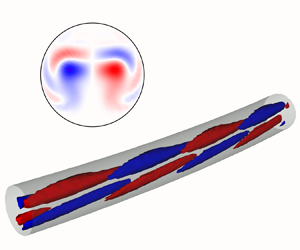
Figure 6. Real part of the critical eigenmode for  $\delta = 10^{-3}$, ${{Re}} = 3575$, $\alpha = 0.338$, belonging to the family of centre modes. Arbitrary scaling of the velocity magnitude. The inner wall of the bend is located on the bottom, whereas the top corresponds to the outer wall.
The global neutral stability curve exhibits a kink at curvatures close to  $1.5 \times 10^{-4}$ since a different family of modes is found at criticality for $1.5 \times 10^{-6} \lessapprox \delta \lessapprox 1.5 \times 10^{-4}$. They are symmetric with respect to the equatorial plane and concentrated mainly in the near-wall region, towards the outer side of the bend. Therefore, they are referred to as wall modes. An example of the spatial structure of these modes is shown in figure 7, which displays the real part of the critical eigenmode for $\delta = 10^{-4}$, ${{Re}} = 5338$ and $\alpha = 1.848$. The wall modes are associated with higher absolute values of the streamwise wavenumber $\alpha$ and the angular frequency $\omega$ than the centre modes. For $\delta \gtrapprox 1.5 \times 10^{-4}$, the neutral stability curve associated with this family of modes shows that they become unstable for higher values of ${{Re}}$ than the centre modes. As stated previously, a higher spatial resolution is employed for tracking wall modes. The need for finer grid spacing is likely ascribed to their spatial structure, which exhibits a thin layer close to the wall.

Figure 7. Real part of the critical eigenmode for  $\delta = 10^{-4}$, ${{Re}} = 5338$, $\alpha = 1.848$, belonging to the family of wall modes. Arbitrary scaling of the velocity magnitude. The inner wall of the bend is located on the bottom, whereas the top corresponds to the outer wall.
For curvatures below approximately  $1.5 \times 10^{-6}$, the critical Reynolds number follows the power-law trend ${{Re}}_{cr} \propto \delta ^{-1/2}$. This result implies that ${{Re}}_{cr}$ diverges to infinity as ${\delta \rightarrow 0}$ and that the Dean number ${{De}} = 2\,{{Re}}\,\sqrt {\delta }$ at criticality is constant, approximately equal to 113, for these values of $\delta$. The critical eigenmodes correspond to the centre modes described above since the wall modes become unstable at higher values of the Reynolds number in this range of curvatures.
For curvatures below approximately  $10^{-4}$, the centre modes exhibit a peculiar behaviour: they become unstable at a certain Reynolds number, and restabilise for higher values of ${{Re}}$, becoming eventually unstable as the Reynolds number is increased further. To better understand this phenomenon, the growth rate associated with this family of modes is computed for several values of $\alpha$ and ${{Re}}$ by means of the generalised Rayleigh quotient iteration. In this way, only the centre modes are tracked.
Neutral stability curves in the  ${{Re}}\unicode{x2013}\alpha$ plane are identified by considering the flow as marginally stable when the absolute value of the computed growth rate is below $10^{-9}$. They are shown in figure 8 for $\delta = 10^{-3}, 10^{-4}, 10^{-5}$. The range of considered streamwise wavenumbers varies depending on the curvature. For $\delta = 10^{-3}$, the centre modes do not restabilise after becoming unstable. On the other hand, for $\delta = 10^{-4}$, a small detached region of instability is observed for $0.135 \lessapprox \alpha \lessapprox 0.185$ and $6200 \lessapprox {{Re}} \lessapprox 7500$. This island of instability arises because the growth rate of the centre modes does not exhibit a monotonic trend with ${{Re}}$ after crossing the marginal stability limit for the considered parameters. Hence, the centre modes become unstable and then restabilise in this region of the parameter space. A similar behaviour is also observed at $\delta = 10^{-5}$ for $0.0375 \lessapprox \alpha \lessapprox 0.0725$. For this value of the curvature, the analysis is also carried out using higher spatial resolution in both radial and azimuthal directions, confirming the robustness of the results. Islands of instability have not been observed by Canton et al. (Reference Canton, Schlatter and Örlü2016), most likely because they are characteristic of low curvatures. Nevertheless, they appear in spiral Couette flow (Meseguer & Marques Reference Meseguer and Marques2000) and spiral Poiseuille flow (Meseguer & Marques Reference Meseguer and Marques2002) as a result of the competition between different instability mechanisms. However, it needs to be remarked that they arise within the same family of modes in the case under investigation.

Figure 8. Neutral stability curves of the centre modes in the  ${{Re}}\unicode{x2013}\alpha$ plane for (a) $\delta = 10^{-3}$, (b) $\delta = 10^{-4}$, (c) $\delta = 10^{-5}$. Shaded areas indicate regions where the base flow is unstable. For all values of the curvature, the computations are performed with $n_r \times n_{\theta } = 25 \times 50$ (blue $\times$ symbols). For $\delta = 10^{-5}$, results for a grid with $n_r \times n_{\theta } = 35 \times 70$ (maroon circles) are also shown.
The streamwise wavenumber  $\alpha$ and the phase speed $v_p = \omega R_p/\alpha$ of the critical modes are reported in figure 9. For curvatures at which centre modes occur at criticality, the streamwise wavenumber exhibits a clear decreasing trend as $\delta$ decreases. In particular, for $\delta \lessapprox 1.5 \times 10^{-6}$, the critical streamwise wavenumber is proportional to the square root of the curvature. According to Trefethen, Trefethen & Schmid (Reference Trefethen, Trefethen and Schmid1999), the least stable mode in a straight pipe occurs for $\alpha \neq 0$. Hence, it is expected that the critical $\alpha$ for toroidal pipes approaches this value smoothly as $\delta \rightarrow 0$. For $\delta \approx 1.5 \times 10^{-6}$ and $\delta \approx 1.5 \times 10^{-4}$, step discontinuities can be observed in the critical streamwise wavenumber since wall modes, characterised by larger absolute values of $\alpha$, are the least stable for $1.5 \times 10^{-6} \lessapprox \delta \lessapprox 1.5 \times 10^{-4}$. For the wall modes, the streamwise wavenumber at criticality decreases as $\delta$ is reduced, but at a lower rate than for centre modes. The wavelength of wall modes is thus less affected by the curvature.

Figure 9. (a) Streamwise wavenumber  $\alpha$ and (b) phase speed $v_p$ of the critical modes as functions of the curvature. Solid lines indicate data for $10^{-7} \leq \delta \leq 10^{-2}$ (computed in the present work), whereas dashed lines show data adapted from Canton et al. (Reference Canton, Schlatter and Örlü2016) for $10^{-2} \leq \delta \leq 1$.
The critical phase speed increases slightly with decreasing curvature for  $1.5 \times 10^{-4} \lessapprox \delta \lessapprox 10^{-2}$, and it exhibits discontinuities at $\delta \approx 1.5 \times 10^{-4}$ and $\delta \approx 1.5 \times 10^{-6}$ due to the switching between the two families of critical modes. For the wall modes, $v_p$ decreases as the curvature is lowered, and its value is close to the amplitude of the base flow streamwise velocity in the region close to the outer wall, where the eigenmodes are predominant. On the other hand, for curvatures below approximately $1.5 \times 10^{-6}$, the phase speed at criticality is almost constant, approximately equal to $1.5 U_b$. Given that the critical modes for $\delta \lessapprox 1.5 \times 10^{-6}$ have their core close to the centre of the pipe, this value of the critical phase speed is not surprising since it is almost equal to the magnitude of the streamwise velocity component of the base flow in this region.
5. Influence of the base flow
The stability analysis of toroidal pipe flows requires the numerical computation of the steady base flow, which increases both the complexity and computational cost of the algorithm. This task can be avoided if a sufficiently accurate eigenvalue spectrum can be obtained using an approximate basic state. In this section, the eigenvalue spectrum computed using different approximate base flows is compared to that obtained by linearising the incompressible Navier–Stokes equations about the numerically computed steady state.
5.1. Semi-analytic base flow
An approximate base flow can be derived by expanding the steady incompressible Navier–Stokes equations in powers of  $\delta$. Considering only the leading-order terms, after some algebraic manipulations, the equations can be written as follows. For the $s$-momentum,
 \begin{align} & \frac{{{De}}}{2 \sqrt{\delta}} \left(r^2 U_s\, \frac{\partial U_r}{\partial r} + r^2 U_r\, \frac{\partial U_s}{\partial r} + r U_r U_s + r U_{{\theta}}\, \frac{\partial U_s}{\partial {\theta}} + r U_s\, \frac{\partial U_{{\theta}}}{\partial {\theta}}\right) \nonumber\\ &\quad - r^2\,\frac{\partial^2 U_s}{\partial r^2} - r\, \frac{\partial U_s}{\partial r} - \frac{\partial^2 U_s}{\partial {\theta}^2} = F\, \frac{{{De}}}{2 \sqrt{\delta}}\,r^2. \end{align}
 For the  $r$-momentum,
 \begin{align} & \frac{{{De}}}{2 \delta} \left(r^2\,\frac{\partial P}{\partial r} + 2 r^2 U_r\, \frac{\partial U_r}{\partial r} + r U_r^2 + r U_{{\theta}}\, \frac{\partial U_r}{\partial {\theta}} + r U_r\, \frac{\partial U_{{\theta}}}{\partial {\theta}} - r U_{{\theta}}^2\right) \nonumber\\ &\quad + \frac{1}{\sqrt{\delta}} \left(2 U_r - r\,\frac{\partial^2 U_{{\theta}}}{\partial r\, \partial {\theta}} - 2 r^2\,\frac{\partial^2 U_r}{\partial r^2} -2 r\,\frac{\partial U_r}{\partial r} - \frac{\partial^2 U_r}{\partial {\theta}^2} + 3\,\frac{\partial U_{{\theta}}}{\partial {\theta}}\right) = 0. \end{align}
 For the  $\theta$-momentum,
 \begin{align} & \frac{{{De}}}{2 \delta} \left(r\,\frac{\partial P}{\partial {\theta} } + r^2 U_{{\theta}}\, \frac{\partial U_r}{\partial r} + r^2 U_r\,\frac{\partial U_{{\theta}}}{\partial r} + 2 r U_r U_{{\theta}} + 2 r U_{{\theta}}\,\frac{\partial U_{{\theta}}}{\partial {\theta} }\right) \nonumber\\ &\quad + \frac{1}{\sqrt{\delta}} \left(U_{{\theta}} - r\,\frac{\partial^2 U_r}{\partial r\,\partial {\theta} } - r^2\, \frac{\partial^2 U_{{\theta}}}{\partial r^2} -r\,\frac{\partial U_{{\theta}}}{\partial r} - 3\, \frac{\partial U_r}{\partial {\theta}} - 2\,\frac{\partial^2 U_{{\theta}}}{\partial {\theta}^2}\right) = 0. \end{align}
The incompressibility constraint is
 \begin{align} & r\,\frac{\partial U_r}{\partial r} + U_r + \frac{\partial U_{{\theta}}}{\partial {\theta}} = 0. \end{align}
 Numerical evidence shows that  $F \propto \sqrt {\delta }$ for a fixed value of ${{De}}$ (see figure 10). Therefore, for a given Dean number, the field $(U_s, U_r/\sqrt {\delta }, U_{{\theta }}/\sqrt {\delta }, P/\delta )^{\rm T}$ is a solution of (5.1) for any combination of $\delta$ and ${{Re}}$.

Figure 10. Amplitude of the volume force  $F$ for steady base flows at ${{De}} = 200$ and different values of the curvature. The dashed line indicates the trend $\sqrt {\delta }$.
The higher-order terms in the expansion can be neglected for curvatures approaching zero, and an approximate steady base flow for a given combination of curvature and Reynolds number can then be derived simply by scaling the solution obtained for different values of  $\delta$ and ${{Re}}$ yielding the same Dean number. This result confirms the conclusion of Canton et al. (Reference Canton, Örlü and Schlatter2017), i.e. that the Dean number similarity does not hold for any value of ${{De}}$, even at low curvatures. It needs to be remarked that the semi-analytic scaling introduced here can be applied only for low curvatures, as in the solution proposed by Dean (Reference Dean1927, Reference Dean1928), but it is valid for any Dean number. Additionally, since the critical Dean number is constant for low curvatures, the proposed scaling implies that the magnitude of the secondary flow at criticality decreases with decreasing $\delta$.
5.1.1. Numerical verification
Numerical computations of steady base flows  $\boldsymbol {Q} = (\boldsymbol {U}, P)^{\rm T}$ for different combinations of $\delta$ and ${{Re}}$ corresponding to the same Dean number support the semi-analytic scaling derived above. Figure 11 shows the absolute value of the difference between the scaled base flows $(U_s, U_r/\sqrt {\delta }, U_{{\theta }}/\sqrt {\delta }, P/\delta )^{\rm T}$ at ${{De}} = 200$ computed for $\delta = 10^{-6}$ and $\delta = 10^{-8}$. The maximum difference between the two cases is of the order of $10^{-5}$. The energy norm of the relative difference between scaled base flows separated by one decade in $\delta$ at ${{De}} = 200$ decays linearly as the curvature decreases, as displayed in figure 12.

Figure 11. Absolute value of the difference of the scaled velocity components and pressure at  ${{De}} = 200$ between the steady base flows at $\delta = 10^{-6}$, ${{Re}} = 10^5$ and $\delta = 10^{-8}$, ${{Re}} = 10^6$, i.e. separated by one order of magnitude in ${{Re}}$. The inner wall of the bend is located on the bottom, whereas the top corresponds to the outer wall.

Figure 12. Energy norm of the relative difference of scaled velocity components and pressure between steady base flows at  ${{De}} = 200$ separated by one decade in $\delta$. The dashed line indicates the linear decay as $\delta$ decreases.
5.2. Eigenvalue spectra
The base flow for low curvatures can be constructed synthetically from previously computed steady solutions by exploiting the semi-analytic scaling described in § 5.1, thus avoiding its explicit numerical computation. However, it is not guaranteed that the accuracy of the base flow asymptotic expansion carries over to the eigenvalue spectrum. Indeed, highly non-normal operators can be significantly affected by small perturbations (Trefethen et al. Reference Trefethen, Trefethen, Reddy and Driscoll1993). The effect on the eigenvalues of having an approximate basic state is thus assessed for  $\delta = 10^{-7}$, ${{Re}} = 500\,000$. Three different approximate basic states are employed in the stability analysis: a base flow built from the solution at $\delta = 10^{-5}$, ${{Re}} = 50\,000$ exploiting the scaling described above, the Hagen–Poiseuille flow (retaining non-zero curvature in the linearised incompressible Navier–Stokes equations), and the numerically computed base flow with in-plane velocity components $U_r$ and $U_{\theta }$ set to zero. The leading eigenvalues for these basic states are reported in figure 13, together with the spectrum for the numerically computed base flow. Using the Hagen–Poiseuille flow as basic state completely fails to capture the spectrum, and considerably unstable eigenvalues are observed. This discrepancy is ascribed to the substantial difference between the base flow at $\delta = 10^{-7}$, ${{Re}} = 500\,000$ and the laminar flow in a straight pipe. Setting the in-plane velocity components to zero in the numerically computed base flow does not provide satisfactory results either. This finding implies that the secondary motion in the basic state has a crucial role in determining the stability properties of the flow, even though it has low intensity (see also Canton et al. Reference Canton, Örlü and Schlatter2017). Nevertheless, as stated above, the magnitude of the secondary flow at criticality decreases as $\delta \rightarrow 0$. Therefore, better agreement is expected for lower curvatures.

Figure 13. Portion of the eigenvalue spectrum for  $\delta = 10^{-7}$, ${{Re}} = 500\,000$, $0.0002 \leq \alpha \leq 0.0155$ computed using different basic states: numerically computed base flow (black $\times$ symbols), Hagen–Poiseuille flow with $\delta \neq 0$ in the linearised Navier–Stokes equations (blue diamonds), base flow derived applying the semi-analytic scaling to the solution for $\delta = 10^{-5}$, ${{Re}} = 50\,000$ (maroon circles), base flow with in-plane velocity components set to zero (green Mercedes star symbols).
No substantial differences are observed between the eigenvalue spectra computed using the scaled basic state and the numerically computed base flow. Hence, the truncation of the asymptotic expansion does not have a significant influence on the stability properties.
It should be pointed out that it is not possible to perform the stability analysis using Dean's expansion of the base flow (Dean Reference Dean1927) since it is valid only for  ${{De}} \ll 37.94$. Thus, it loses any meaning at criticality, where ${{De}}_{cr} \approx 113$. Indeed, at Dean numbers as high as those on the global neutral stability curve, the base flow derived by Dean exhibits reversed flow, which is not physical in the considered configuration. However, the semi-analytic scaling described in § 5.1 can be applied in these cases.
6. Discussion and outlook
The present work extends the modal stability analysis of toroidal pipe flows carried out by Canton et al. (Reference Canton, Schlatter and Örlü2016) to values of the curvature  $\delta$ approaching zero, i.e. a straight pipe. The global neutral stability curve is traced through a continuation algorithm. Because of the properties of the geometry, the critical modes are either symmetric or antisymmetric with respect to the equatorial plane, depending on the value of the curvature. Although the flow in a toroidal pipe undergoes subcritical transition for $\delta \lessapprox 0.028$, the present work highlights that the critical Reynolds number for modal instability diverges to infinity as the curvature approaches zero. The Dean number at criticality is approximately equal to 113 for low curvatures. For sufficiently low values of $\delta$, the streamwise wavenumber of the critical mode is proportional to $\sqrt {\delta }$, whereas the critical phase speed plateaus at a value of approximately $1.5 U_b$. These findings constitute further proof of the fact that the Hagen–Poiseuille flow is indeed stable to infinitesimal disturbances for any Reynolds number, as stated by Meseguer & Trefethen (Reference Meseguer and Trefethen2003) based on stability calculations. They also indicate a continuous transition of the stability properties of curved pipe flows towards the straight pipe limit.
The influence on the eigenvalue spectrum of having an approximate base flow is also investigated. Asymptotic expansions, corroborated by numerical evidence, show that the field  $(U_s, U_r/\sqrt {\delta }, U_{{\theta }}/\sqrt {\delta }, P/\delta )^{\rm T}$ is an approximate self-similar solution of the steady incompressible Navier–Stokes equations for any combination of $\delta$ and ${{Re}}$ corresponding to a fixed Dean number. The error of the approximation is found to be negligible for very low curvatures. For a given Dean number, an approximate base flow can then be derived from a solution at different curvature and Reynolds number. For $\delta = 10^{-7}$ and ${{Re}} = 500\,000$, this approximate basic state provides an eigenvalue spectrum in good agreement with that obtained using the numerically computed base flow. On the other hand, using the Hagen–Poiseuille flow as basic state and retaining non-zero curvature in the linearised incompressible Navier–Stokes equations does not yield accurate results, implying that the secondary flow is pivotal in the stability analysis. Neither does the stability analysis for the numerically computed base flow with the in-plane velocity components set to zero correctly capture the eigenvalue spectrum, confirming this finding.
Finally, it is worth mentioning that a validation of the present results by means of direct numerical simulations or experiments is not straightforward. Indeed, assuming that one can eliminate all the disturbances leading to subcritical transition, a complete torus of length  $L_t = 2 {\rm \pi}R_p/\delta$ needs to be investigated in order not to miss any potentially relevant wavenumber. Considering an experimental facility consisting of a pipe with cross-section diameter 1 m (the pipe facility at CICLoPE has diameter 90 cm; see Örlü et al. Reference Örlü, Fiorini, Segalini, Bellani, Talamelli and Alfredsson2017), a complete torus with curvature $\delta = 10^{-7}$ will have length approximately 31 000 km, which is of the same order of magnitude of Earth's circumference (approximately 40 000 km).
Acknowledgements
Computer time provided by the Swedish National Infrastructure for Computing (SNIC) is acknowledged.
Funding
This research was funded by the Swedish Research Council (VR) under grant no. 2017-04421.
Declaration of interests
The authors report no conflict of interest.
Appendix A. Linearised incompressible Navier–Stokes equations in toroidal coordinates
This appendix presents the incompressible Navier–Stokes equations linearised about the steady state  $\boldsymbol {Q} = (\boldsymbol {U}, P)^{\rm T}$ and expressed in toroidal coordinates. The perturbation fields are indicated by $(\boldsymbol {u}', p')^{\rm T} = (u_s', u_r', u_{\theta }', p')^{\rm T}$.
For the  $s$-momentum,
 \begin{align} & \frac{\partial u_s'}{\partial t}+\left[ -\frac{1}{r^2\,{{Re}}}\,\frac{\partial^2 }{\partial {\theta}^2} + \frac{2 \delta \cos({\theta})\,{U_{\theta}}}{\delta r \sin({\theta}) + 1} + \frac{\partial U_r}{\partial r} + \frac{3}{r}\,U_r + \frac{1}{r}\, \frac{\partial U_{\theta}}{\partial {\theta}} - \frac{2 {U_r}}{r(\delta r \sin({\theta}) + 1)}\right. \nonumber\\ &\quad \left.{}+ \frac{\delta^2 }{{{Re}}\,(\delta r \sin({\theta}) + 1)^2} + \left( {U_r} + \frac{1}{r\,{{Re}}\,(\delta r \sin({\theta}) + 1)} -\frac{2}{r\,{{Re}}}\right) \frac{\partial}{\partial r}\right. \nonumber\\ &\quad \left.{}+\left( \frac{U_{\theta}}{r} - \frac{\delta \cos({\theta})}{r\,{{Re}}\,(\delta r \sin({\theta}) + 1)}\right) \frac{\partial}{\partial {\theta}}-\frac{2}{{{Re}}\,(\delta r \sin({\theta}) + 1)^2}\, \frac{\partial^2 }{\partial s^2}-\frac{1}{{{Re}}}\,\frac{\partial^2 }{\partial r^2}\right. \nonumber\\ &\quad \left.{}+ \frac{2 {U_s}}{\delta r \sin({\theta}) + 1}\,\frac{\partial}{\partial s}\right] u_s' + \left[ \frac{1}{r\,{{Re}}} \left(\frac{3}{(\delta r \sin({\theta}) + 1)^2} - \frac{4}{\delta r \sin({\theta}) + 1}\right) \frac{\partial}{\partial s} \right. \nonumber\\ &\quad \left.{}+\frac{\partial U_s}{\partial r} - \frac{2 {U_s}}{r (\delta r \sin({\theta}) + 1)} + \frac{3}{r}\,{U_s}-\frac{1}{{{Re}}\,(\delta r \sin({\theta}) + 1)}\, \frac{\partial^2}{\partial s\,\partial r}+ {U_s}\,\frac{\partial}{\partial r} \right] u_r' \nonumber\\ &\quad +\left[ \frac{2 \delta \cos({\theta})\,{U_s}}{\delta r \sin({\theta}) + 1} + \frac{1}{r}\, \frac{\partial U_s}{\partial {\theta}}-\frac{1}{r\,{{Re}}\,(\delta r \sin({\theta}) + 1)}\, \frac{\partial^2}{\partial s\,\partial {\theta}}\right. \nonumber\\ &\quad \left.{}-\frac{3 \delta \cos({\theta})}{{{Re}}\,(\delta r \sin({\theta}) + 1)^2}\, \frac{\partial}{\partial s}+\frac{{U_s}}{r}\,\frac{\partial}{\partial {\theta}} \right] u_{\theta}' + \frac{1}{\delta r \sin({\theta}) + 1}\,\frac{\partial p'}{\partial s} = 0. \end{align}
 For the  $r$-momentum,
 \begin{align} & \frac{\partial u_r'}{\partial t}+\left[\left(\frac{{U_r}}{\delta r \sin({\theta}) + 1} + \frac{3}{r\,{{Re}}\,(\delta r \sin({\theta}) + 1)} - \frac{3}{r\,{{Re}}\, (\delta r \sin({\theta}) + 1)^2}\right)\frac{\partial }{\partial s}\right. \nonumber\\ &\quad \left.{}+\frac{2 {U_s}}{r(\delta r \sin({\theta}) + 1)}-\frac{2}{r}\,{U_s} -\frac{1}{{{Re}}\,(\delta r \sin({\theta}) + 1)}\,\frac{\partial^2}{\partial s\,\partial r} \right] u_s' \nonumber\\ &\quad +\left[\frac{1}{r^2\,{{Re}}\,(\delta r \sin({\theta}) + 1)^2}\left(2 + r\,{{Re}}\, (\delta r \sin({\theta}) + 1) \left((\delta r \sin({\theta}) + 1) \left(2 r\,\frac{\partial U_r}{\partial r}\right .\right. \right. \right. \nonumber\\ &\quad \left. \left. \left. \left.{}+\frac{\partial U_{\theta}}{\partial {\theta}}\right) + (4\,\delta r \sin({\theta}) + 2) {U_r} + \delta r \cos({\theta})\,{U_{\theta}}\right) + 4\, \delta r \sin({\theta})\,(\delta r \sin({\theta}) + 1)\right)\right. \nonumber\\ &\quad \left.{}+\left(2 {U_r} + \frac{2}{r\,{{Re}}\,(\delta r \sin({\theta}) + 1)} - \frac{4}{r\,{{Re}}}\right) \frac{\partial}{\partial r} - \frac{1}{r^2\,{{Re}}}\, \frac{\partial^2}{\partial {\theta}^2} +\frac{{U_s}}{\delta r \sin({\theta}) + 1}\, \frac{\partial}{\partial s}\right. \nonumber\\ &\quad \left.{}+\left(\frac{U_{\theta}}{r} - \frac{\delta \cos({\theta})}{r\,{{Re}}\, (\delta r \sin({\theta}) + 1)}\right) \frac{\partial}{\partial {\theta}} -\frac{1}{{{Re}}\,(\delta r \sin({\theta})+1)^2}\,\frac{\partial^2}{\partial s^2} -\frac{2}{{{Re}}}\,\frac{\partial^2}{\partial r^2}\right] u_r' \nonumber\\ &\quad +\left[ \left(\frac{1}{r}\,\frac{\partial U_r}{\partial {\theta}} + \frac{\delta \cos({\theta})\,(r\,{{Re}}\,{U_r}+3)}{r\,{{Re}}\, (\delta r \sin({\theta}) + 1)} - \frac{2}{r}\,{U_{\theta}} - \frac{2 \delta \cos({\theta})}{r\,{{Re}}\,(\delta r \sin({\theta}) + 1)^2}\right)\right. \nonumber\\ &\quad \left.{}+ \left(\frac{U_r}{r} + \frac{3}{r^2\,{{Re}}} \right)\frac{\partial}{\partial {\theta}} -\frac{\delta \cos({\theta})}{{{Re}}\,(\delta r \sin({\theta}) + 1)}\, \frac{\partial}{\partial r}-\frac{1}{r\,{{Re}}}\,\frac{\partial^2}{\partial r\,\partial {\theta}}\right] u_{\theta}' + \frac{\partial p'}{\partial r} = 0. \end{align}
 For the  $\theta$-momentum,
 \begin{align} & \frac{\partial u_{\theta}'}{\partial t}+\left[ \left(\frac{{U_{\theta}}}{\delta r \sin({\theta}) + 1} + \frac{3 \delta \cos({\theta})}{{{Re}}\,(\delta r \sin({\theta})+1)^2}\right) \frac{\partial}{\partial s}\right. \nonumber\\ &\quad \left.{}-\frac{1}{r\,{{Re}}\,(\delta r \sin({\theta}) + 1)}\, \frac{\partial^2}{\partial s\,\partial {\theta}}-\frac{2 \delta \cos({\theta})\, {U_s}}{\delta r \sin({\theta})+1} \right] u_s' \nonumber\\ &\quad +\left[\frac{1}{r^2\,{{Re}}}\left(\frac{1}{\delta r \sin({\theta})+1} - 4\right) \frac{\partial}{\partial {\theta}}+ \frac{\partial U_{\theta}}{\partial r} - \frac{{U_{\theta}}}{r(\delta r \sin({\theta}) + 1)} + \frac{3}{r}\,{U_{\theta}}\right. \nonumber\\ &\quad \left.{}- \frac{2 \delta \cos({\theta})}{r\,{{Re}}\,(\delta r \sin({\theta})+1)^2} -\frac{1}{r\,{{Re}}}\,\frac{\partial^2}{\partial r\,\partial {\theta}} + {U_{\theta}}\,\frac{\partial}{\partial r} \right] u_r' \nonumber\\ &\quad +\left[\frac{2 \delta \cos({\theta})\,{U_{\theta}}}{\delta r \sin({\theta}) + 1} + \frac{1}{r} \left(r\,\frac{\partial U_r}{\partial r} + 3 {U_r} + 2\, \frac{\partial U_{\theta}}{\partial {\theta}}\right) - \frac{{U_r}}{r(\delta r \sin({\theta}) + 1)} \right. \nonumber\\ &\quad \left.{}+ \frac{2 \delta ^2}{{{Re}}\,(\delta r \sin({\theta}) + 1)^2} + \frac{1}{r^2\,{{Re}}}\left(\frac{3}{\delta r \sin({\theta}) + 1} - \frac{2}{(\delta r \sin({\theta})+1)^2}\right)-\frac{2 }{r^2\,{{Re}}}\, \frac{\partial^2}{\partial {\theta}^2}\right. \nonumber\\ &\quad \left.{}+\left({U_r} + \frac{1}{r\,{{Re}}\,(\delta r \sin({\theta}) + 1)} - \frac{2}{r\,{{Re}}}\right) \frac{\partial}{\partial r}+\left(\frac{2}{r}\,{U_{\theta}} - \frac{2 \delta \cos({\theta})}{r\,{{Re}}\,(\delta r \sin({\theta}) + 1)}\right) \frac{\partial}{\partial {\theta}}\right. \nonumber\\ &\quad \left.{}-\frac{1}{{{Re}}\,(\delta r \sin({\theta}) + 1)^2}\,\frac{\partial^2}{\partial s^2} -\frac{1}{{{Re}}}\,\frac{\partial^2}{\partial r^2} +\frac{{U_s}}{\delta r \sin({\theta}) + 1}\,\frac{\partial}{\partial s} \right] u_{\theta}' + \frac{1}{r}\,\frac{\partial p'}{\partial {\theta}} = 0. \end{align}
The incompressibility constraint is
 \begin{align} & \left[ r\,\frac{\partial}{\partial s}\right] u_s' +\left[(2 \delta r \sin({\theta})+1) + r (\delta r \sin({\theta}) + 1)\, \frac{\partial}{\partial r}\right] u_r' \nonumber\\ &\quad + \left[ \delta r \cos({\theta}) + (\delta r \sin({\theta}) + 1)\, \frac{\partial }{\partial {\theta}}\right] u_{\theta}' = 0. \end{align}


 Open access