


1. Introduction
To understand the global climate system it is necessary to st Lilly ice-occan-atmosphere inleraclions over the Southern Ocean, which occupies a large area and links the world's major oceans. One of the key elements of the Southern Ocean is sea ice. Sea-ice concentrations have been observed from satellite and analyzed by many researchers. 7.wally and others (1983) and Reference ParkinsonParkinson (1995) showed that sea-ice concentration exhibits large interannual variability, making climatic trends difficult to determine. Reference Murphy, Clarke, Symon and PriddleMurphy and others (1995) confirmed this variability from fast-ice data in the South Orkney Islands and found that anomalies in sea-ice extent show an eastward propagation around the Antarctic continent with a period of approximately 7-9 years. Murphy and others (1995) also indicated that the interannual variability of Antarctic sea ice is closely related to El Niño Southern Oscillation (ENSO) events. Reference GloersenGloersen (1995) showed that time series of sea-ice cover over the Southern Ocean contain statistically significant quasi-biennial and quasi-quadrennial periodicities which agree well with variations in the ENSO index.
White and Peterson (1996) found that the interannual variability of sea ice over the Southern Ocean reflects interannual variability of the ocean atmosphere coupled system including sea-level pressure (SLP), wind stress and sea-surface temperature (SST). This coupled system is referred to as the Antarctic Circumpolar Wave (ACW). Reference Jacobs and MitchellJacobs and Mitchell (1996) analyzed altimeter data and found that sea-surface height (SSH) anomalies vary with the ACW The SSH response to observed wind forcing is also explained with simple quasi-gcostrophic dynamics by Jacobs and Mitchell (1996).
In the present study, the ACW is investigated with a global coupled ocean-atmosphere model. The ACW appears during the 150 year integration of the model.
2. Model Description
The atmospheric component of the coupled model is a new version of the MRI GCM-I (Reference Tokioka, Yamazaki, Yagai and KitohTokioka and others, 1984) and includes a diurnal cycle. The horizontal resolution is 4° in latitude and 5° in longitude. There are 15 hybrid layers between the surface and the model top at 1 hPa. The atmospheric model and its performance are described in detail by Kitoh and others (1995).
The ocean component of the coupled model was developed at the Meteorological Research Institute, Ibaraki, Japan. It is based on the ocean general circulation model of Reference BryanBryan (1969) and includes the Reference Mellor and YamadaMellor and Yamada (1974) level 2 turbulence closure scheme. The horizontal resolution is 2 in latitude and 2.5° in longitude with in the global domain except in the equatorial region between 12° N and 12° S. Here, the horizontal resolution is refined in the north-south direction in order to resolve equatorial waves and thus simulate El Nino events. The resolution is 0.5 in latitude with in the 4° N-4° S band. Between 4° N(S) and 12° N(S) the grid spacing varies almost linearly from 0.5° to 2° in latitude. The bottom topography and coastline are represented realistically on a scale consistent with model resolution. The vertical layers of the ocean model vary in thickness to give more resolution near the surface. There are 21 layers, which thicken from 5.2 m to 700 m in the vertical direction, with 11 layers in the top 300 m.
The sea-ice model used in the coupled model is similar to that of Mellor and Kanlha (1989) in terms of the thermodynamics. The prognostic variables are sea-ice thickness and concentration. The model solves the equations for conservation of mass and concentration by taking into account the freeze or melt rate at the bottom of the sea ice, the freeze rate in leads (open water), the rate of sea-ice accretion at the sea surface due to frazil-ice formation and the melt rate at the surface.

Fig. 1. Time-longitude diagrams of sea-surface temperature anomalies (SSTA) and sea-surface salinity anomalies (SSSA) along 56° S in the model. Negative anomalies are shaded. Contour intervals are 0.3°C for SSTA and 0.1psu for SSSA.
3. Method of Coupling Atmospheric, Ocean and Sea-Ice Models
With in the coupling interval of 6 hours, the atmospheric model runs with sea-surface temperature and velocity, sea-ice thickness and concentration, and temperature at the bottom of the sea ice all fixed. Relevant time-mean fluxes of momentum, heat and fresh water are then accumulated. These fluxes are used to drive the corresponding 6 hour integration of the ocean and sea-ice models. These then provide updated sea-surface temperatures and velocities, sea-ice thicknesses and concentrations, and temperatures at the bottom of the sea ice which are fed back to the atmospheric model for the next coupling interval. The atmospheric model uses 1 hour time-steps, and the ocean and sea-ice models use 30 min time-steps.
4. Experimental Procedure
The atmospheric model is spun up for 3 years using observed sea-surface temperatures and sea-ice distribution. The ocean model is spun up (using an accelerating method described by Bryan (1984)) for 1500 years, using the surface fluxes obtained during the spin-up of the atmosphere. The temperatures and salinities at the uppermost layer are relaxed toward climatological sea-surface temperatures (SSTs) and salinities (SSSs). After the spin-up of the atmosphere and ocean, the coupled model (including the sea-ice model) is then spun up for 30 years. A flux adjustment for heat and fresh water is obtained during the last 10 years of the 30 year spin-up. The fully coupled model is then integrated for 150 years using the derived llux adjustments.

Fig. 2. (a) Spatial patterns and (b) time coefficients for EOF1 of SST in the model (explains 30.3% of total variance). (c,d) Asfor (a) and (b) except for observations (explains 46.1% of total variance).
5. Results
Time-longitude diagrams of interannual anomalies in the SSTand SSS along 56° S from model years 51-95 are shown in Figure 1. The eastward propagation of the anomalies is clearly identified as an ACW in the model. It lakes 20-30 years to encircle the pole, which is 2-3 times longer than indicated by observations. The reason for the slower propagation of the anomalies is that the speed of the Antarctic Circumpolar Current (ACC) is lower in the model than in the observations. The mean speed of the ACC is about 0.02 m s−1 in the model, nearly the same as the propagation speed of the anomalies, indicating that advection is important. The amplitude of the anomalies is 1.2°C in SSTand 0.4 psu in SSS. The amplitude in SST agrees with observations (Whiteand Peterson, 1996). Saline (fresh) anomalies correspond to warm (cold) anomalies, as mentioned by Murphy and others (1995).

Fig. 3. Time longitude diagrams of sea-ice concentration anomalies (SICA) and sea-ice thickness anomalies (SITA) along 64°S in the model. Positive anomalies are shaded. Contour intervals are 5% for SICA and 5 cm for SITA.
figure 2a and b show the spatial patterns and time coefficients for EOF1 of interannual SST in the model. The spatial patterns are indicated by correlation coefficients between raw values and the time series. This leading mode represents 30.3% of the total variance. figure 2c and d show the corresponding result for observed SST (GISST2.2, compiled by the U.K. Meteorological Olficc; Reference Rayner, Folland, Parker and HortonRayner and others, 1995). This mode explains 46.1% of the total variance. The coherent variations over the Southern Ocean are similar in the model results and the observations. The wavenumber 2 signal in the Southern Ocean represents one phase of the propagating ACW Note that the full scale of time in figure 2b is 70 years but that in figure 2d is 12 years.

Fig. 4. Distribution of anomalies in density (top) and velocity (bottom) in the Southern Ocean at a depth of 110 m for year 91.
There is high coherence between the ACW and El Niño. The time series in figure 2d clearly shows El Niño in 1982-83,1987 and 1991-94 and La Niña in 1984-85 and 1988-89. The warmest SST appears over the eastern Pacific sector of the Southern Ocean as an ACW signal when the El Niño is at a mature stage. There is a St rong relationship between the ACW and the ENSO, as mentioned by Gloersen (1995) and Murphy and others (1995).
Time-longitude diagrams of sea-ice concentration anomalies (SICA) and sea-ice thickness anomalies (SITA) along 64° S are shown in Figure 3. These indicate that the sea-ice anomalies also propagate eastward around the Antarctic continent with the SSTand SSS anomalies. Sea-ice formation is suppressed (enhanced) southward of warm (cold) and saline (fresh) surface-water areas. These results agree with the observed relationship between fast-ice duration and sea-water temperature at local stations in the South Orkney Islands reported by Murphy and others (1995). Figure 3 also shows that high sea-ice concentration anomalies correspond well to thick sea-ice anomalies. The range of anomalies is as large as 30% in SICA and 20 cm in SITA.
The ACC has clockwise (counter-clockwise) geostrophic velocity anomalies over high- (low-)density anomaly regions. Figure 4 shows the distribution of both density and velocity anomalies at a depth of 110 m for year 91 in the model. High-density anomalies occupy two opposite regions in the Southern Ocean. High-density regions due to upwelling correspond dynamically to low-SSH regions. Clockwise velocity anomalies can be detected over high-density anomaly areas with geostrophic consistency.

Fig. 5. Time-longitude diagrams of density anomalies (DA) and meridional current anomalies (VA) along 56°S in the model. Negative anomalies are shaded. Contour intervals are 0.02 kg m−3 for DA and 0.05 cm S−1 for VA.
Figure 5 shows time-longitude diagrams of anomalies in density and meridional current at a depth of 110 m along 56° S in the model. It is clear that the density anomalies propagate eastward with the ACW. Since the high-density anomalies correspond to low-SSH anomalies, this result suggests propagation of SSH anomalies and supports the data analyses ofjacobs and Mitchell (1996). Comparing the density anomalies in Figure 5 to the SSTand SSS anomalies in Figure 1, it is clear that the density anomalies are produced by salinity anomalies at 56° S. This is reasonable according to the equation of stale for sea water. Salinity is the controlling factor in the density of sea water with in the polar ocean. Thus salinity is indispensable for understand-ing the mechanism of the ACW. The poleward current anomalies shaded in Figure 5 occur at transient zones from low- to high-density anomalies with geostrophic consistency.
A time-longitude diagram of SLP anomalies along 54° S is shown in Figure 6 which indicates propagation eastward with the ACW. The amplitude of the SLP anomalies is about 2 hPa which is smaller than that seen in observations (see White and Peterson, 1996). The high-SLP anomalies correspond to low-density anomalies in the ocean. The counterclockwise wind-stress anomalies with high-SLP anomalies could induce convergence in the Ekman layer with down-welling, resulting in low-density anomalies which dynamically correspond to high-SSH anomalies.

Fig. 6. Time-longitude diagram of sea-level pressure anomalies (SLPA) along 54° S in the model. Negative anomalies are shaded. Contour interval is 1hPa.
6. Summary and Conclusions
An ACW is simulated with a global coupled ocean—atmosphere model. Time-longitude diagrams of anomalies in SS Tand SSS show anomalies propagate eastward. The time taken to encircle the pole is 20-30 years, which is 2-3 times longer than indicated by observations. The reason for the slower propagation speed is that the speed of the simulated ACC is lower than indicated by observations. The mean current speed in the ACC is about 0.02 ms−1 in the model, nearly the same as the propagation speed of the simulated ACW, indicating that advection due to the ACC is important. High-SSS anomalies correspond to high-SST anomalies, high-density anomalies and thus low-SSH anomalies, indicating that salinity is a dominant factor for ocean dynamics in the Southern Ocean. Sea-ice formation is suppressed southward of warm-, saline-water regions and enhanced southward of cold-, fresh-water regions. High sea-ice concentration anomalies correspond to thick sea-ice anomalies.
EOF analysis of SST anomalies shows that the dominant pattern is characterised by wavenumber 2 (180° of longitude wavelength) in the Southern Ocean. The spatial pattern and time series are similar to the dominant EOFof observed anomalies, suggesting that the ACW is closely related to El Niño activity. The simulated ACC has clockwise geostrophic velocity anomalies over high-density anomaly regions. SLP anomalies propagate eastward with the ACW, with high-SLP anomalies corresponding to low-density anomalies.
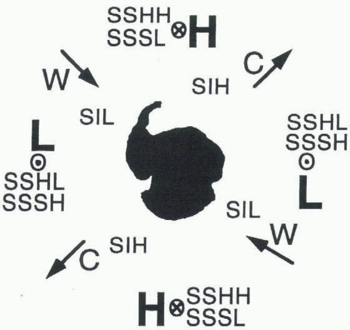
Fig. 7.
A schematic view of the ACW with high (low) anomalies in sea-level pressure indicated by H (L), sea-surface height by SSHH (SSHL) sea-surface salinity by SSSH (SSSL), sea-surface temperature by w(C) and sea ice by SIH (SIL). Upwelling (![]() ), downwelling (
), downwelling (![]() ) and geostrophic current (
) and geostrophic current (![]() ) indicate anomalous advection.
) indicate anomalous advection.
The coupled system of ocean and atmospheric anomalies associated with the ACW is summarized in Figure 7, with positive (negative) anomalies in SLP denoted as H (L), SSH as SSHH (SSHL), SSS as SSSH (SSSL), SST as w(C) and sea ice as SIH (SIL). Upwelling ![]() downwelling
downwelling ![]() and geostrophic current anomalies
and geostrophic current anomalies ![]() are also shown. The counter-clockwise wind-stress anomalies with high-SLP anomalies cause convergence in the Ekman layer with downwelling, resulting in low-density anomalies which correspond to high-SSH anomalies. The downwelling induces the low-SSS and -SSTanomalies through weak transport of salt and heat from the saline, warm deep water.
are also shown. The counter-clockwise wind-stress anomalies with high-SLP anomalies cause convergence in the Ekman layer with downwelling, resulting in low-density anomalies which correspond to high-SSH anomalies. The downwelling induces the low-SSS and -SSTanomalies through weak transport of salt and heat from the saline, warm deep water.
High-SSH anomalies cause counter-clockwise geostrophic velocity anomalies and thus anomalous horizontal advection of heat and salt which influence SST, SSS and sea-ice anomalies. Sea-ice formation is suppressed in the warm, saline region because the excess heat needs to be released and excess salt causes deeper convection which entrains heat from the deep layer.
Acknowledgements
The authors wish to thank their colleagues in the Meteorological Research Institute for informative discussions. We are grateful to W. L. Chan for his comments on a draft of the manuscript. Thanks are also extended to I. N. Smith and many other editors for their helpful advice. We also thank two anonymous reviewers for constructive and useful comments.


