


1. Introduction
Many biomedical devices are designed to minimise local flow recirculation to avoid the trapping of undesirable biological solutes/agents and debris and/or enhance washout of such solutes. For example, vortices resulting from blood flow through arterial stents can serve as accumulation sites for inflammatory elements, leading to arterial thrombosis, and a streamlined stent strut design is recommended to reduce regions of closed streamlines (Jiménez & Davies Reference Jiménez and Davies2009). Additionally, inducing three-dimensional (3-D) spiral flow through the stented region of an artery has been shown to enhance washout through the clearance of recirculation zones (Coppola & Caro Reference Coppola and Caro2009; Xhang et al. Reference Xhang, Tkatch, Newman, Grimme, Vainchtein and Kresh2019). The trapping of debris within regions of vortical flow is also undesirable in medical imaging procedures such as endoscopy or optical coherence tomography. In these procedures, flushing with saline or a contrast agent is used to remove biological debris and blood, respectively, and consequently to enhance visualisation.
Recirculating vortices and the associated mass transport also have a number of applications in cleaning and decontamination processes (see Min, Fischer & Pearlstein (Reference Min, Fischer and Pearlstein2020) and references therein). During the removal of the chemical agents used in these processes, agents can be trapped in the neighbourhood of, or adsorbed onto, the rough surface of the object being cleaned. To investigate the role of rough surface topography on the boundary layer flow of contaminant, Min et al. (Reference Min, Fischer and Pearlstein2020) considered the fluid flow over a backward-facing step and the associated mass transport properties of a passive scalar. Recirculation regions were found adjacent to the vertical face of the step, and the study revealed a subtle interplay between the advective and diffusion transport mechanisms of a passive scalar.
In many biomedical devices, recirculation regions of flow arise as a result of flow into or out of cavities (Clavica et al. Reference Clavica, Zhao, ElMahdy, Drake, Zhang and Carugo2014; Williams et al. Reference Williams, Castrejon-Pita, Turney, Farrell, Tavener, Moulton and Waters2020). Here, we draw particular motivation from urological examples. In ureteroscopy, a minimally invasive procedure for kidney stone removal, a long thin ureteroscope, which contains a hollow tube called the working channel, is inserted through the urinary tract and into the renal pelvis, the hollow cavity within the kidney. Dust-like fragments of kidney stones – which are broken up using thermal energy introduced via high-frequency laser pulses – are cleared from the kidney by a continuous flow of irrigation fluid through the working channel tip and into the kidney. The fluid exits the body in the opposite direction, along the outside of the scope shaft. In ureteroscopy, visualisation is provided to the clinician via a small light and camera embedded in the scope tip, and thus a rapid and thorough clearing of kidney stone dust is important for maintaining a clear field of view. Another urological example of cavity flow recirculation affecting debris clearance occurs when the kidney stone blocks the ureter, which connects the bladder to the renal pelvis, and a urinary stent – a hollow tube with sideholes in the wall to permit the transport of fluid between the intra- and extraluminal spaces – is deployed to promote drainage. In the neighbourhood of a stone, the extraluminal region takes the form of a closed cavity with flow entering via a stent sidehole and exiting along the extraluminal outflow. The development of recirculating regions/vortices causes particles (stone crystals and bacteria) to become trapped before they are washed away, resulting in stent encrustation and potential stent failure (Clavica et al. Reference Clavica, Zhao, ElMahdy, Drake, Zhang and Carugo2014). Percutaneous nephrolithotomy provides yet another urological example. In this procedure, kidney stones too large to be removed using minimally invasive procedures such as ureteroscopy are manually extracted with a nephroscope which is inserted into the patient's kidney via an abdominal incision. As with ureteroscopy, continuous irrigation is required to wash residual stone particles from the kidney. A previous numerical and experimental study examined the effects of irrigation flow speed and nephroscope angle (with respect to the bottom of the treated calyx) on particle clearance rate (Paster et al. Reference Paster, Shlain, Barghouthy, Liberzon, Aviram and Sofer2019). It was found that clearance was most efficient with the nephroscope positioned perpendicularly to the bottom of the calyx using the fastest tested flow speed.
Consideration of such cavity flows motivates the question of how best to design the device and/or the procedure to minimise the washout time of biological debris. We recently considered cavity flow and washout in a 2-D cavity with inlet and outlet channels modelling fluid flow with the steady incompressible Navier–Stokes equations (Williams et al. Reference Williams, Castrejon-Pita, Turney, Farrell, Tavener, Moulton and Waters2020). We demonstrated the presence of symmetry breaking in the flow structure with increasing Reynolds number, such that the asymmetric flow observed at higher Reynolds numbers is dominated by a large central vortex. When incorporating washout of a passive tracer via advection and diffusion, we found a strong link between washout time and the presence, size and location of vortices. This result fits a general trend: the time required for a passive tracer to exit regions of closed streamlines in a steady flow scales both with the size of the vortex and with decreasing diffusion coefficient of the tracer (Rhines & Young Reference Rhines and Young1983). Thus, for fixed diffusive properties, decreasing the size of vortices is paramount for reduction in washout time (Abergel & Temam Reference Abergel and Temam1990).
In this paper we reveal how alternative shapes for the inflow and outflow channels can be used to enhance the clearance of a passive tracer, and we determine the inflow and outflow channel geometries for which the washout time of an initial concentration of passive tracer is minimised. We approach this question using shape optimisation techniques, which rely on the identification of an appropriate objective to minimise. Ideally, the objective would be the washout time for a given initial concentration of tracer. However, such an objective depends upon features of both the flow and the concentration fields, and thus optimisation presents a computationally prohibitive task: even if we consider a steady flow field which is unaffected by the motion of the tracer, computing the washout for any given shape requires solving the fluid equations and subsequently solving a transient advection–diffusion problem for the motion of the tracer. Instead, to define a tractable shape optimisation problem, we determine an objective that is purely based on properties of the steady flow field, but which correlates with washout time.
As noted, we expect the size of vortices to serve as a useful proxy for washout time, and thus base our objective on the size of vortical regions, though quantifying the presence of vortices is in itself a non-trivial pursuit. A logical choice would be to consider vorticity magnitude (Jeong & Hussain Reference Jeong and Hussain1995). This has been previously used as an objective in shape optimisation to reduce recirculation zones (Abergel & Temam Reference Abergel and Temam1990), although more recently objectives which focus on properties of the determinant of the velocity gradient have been shown to achieve superior results (Kasumba & Kunisch Reference Kasumba and Kunisch2010, Reference Kasumba and Kunisch2012). For a given flow field  $\boldsymbol {u}$, vortices are characterised by regions where $\det \boldsymbol {\nabla }\boldsymbol {u} > 0$ (Jeong & Hussain Reference Jeong and Hussain1995). Thus, integrating a smooth form of $\max (0, \det \boldsymbol {\nabla }\boldsymbol {u})$ over the desired domain provides an objective that can be used with a shape optimisation algorithm to determine the optimal inflow and outflow channel shapes to minimise recirculation zones (Kasumba & Kunisch Reference Kasumba and Kunisch2012). We employ such an objective and compute optimal shapes over a range of fluid properties, characterised by Reynolds number. We then confirm that this objective correlates well with washout time across the range of parameters tested, including the diffusivity of tracer particles, and show that the optimised channel shapes can provide a significant decrease in washout time.
2. Problem description
We consider a simplified, 2-D representation of inflow and outflow to/from a rectangular cavity, though we also briefly explore channel optimisation for different cavity geometries in § 4. This set-up is motivated by an idealisation of a ureteroscope tip within the renal pelvis, but more generally provides a toy geometry for considering shape optimisation on flows characterised by large vortical structures. We employ a Cartesian coordinate system  $(x^{\star }, y^{\star })$ (stars indicate dimensional variables throughout) with corresponding coordinate directions $\boldsymbol {i}$ and $\boldsymbol {j}$.
The flow domain is represented by the light pink and light orange regions in figure 1, i.e.  $\varOmega _{{t}}^{\star }\cup \varOmega _{{c}}^{\star }$. The $\varOmega _{{t}}^{\star }$ domain encompasses both inflow and outflow channels. The inflow boundary to the working channel is $\varGamma ^{\star }_{{in}}$, the upper and lower outflow boundaries are $\varGamma ^{\star }_{{out,u}}$ and $\varGamma ^{\star }_{{out,l}}$, respectively, $\varGamma ^{\star }_{{f}}$ is the solid boundary we will allow to vary in the shape optimisation and $\varGamma ^{\star }_{{wall}}$ denotes all other (fixed) solid boundaries. Following on from our previous experimental and numerical work in a similar geometry (Williams et al. Reference Williams, Castrejon-Pita, Turney, Farrell, Tavener, Moulton and Waters2020), we use the parameter values $l_1=1.2743\ \text {cm}$ and $l_2 = 1\ \text {cm}$ for the channel and cavity lengths, respectively, and set $a = 0.06\ \text {cm}$, $b = 0.25701\ \text {cm}$ and $h=0.11598\ \text {cm}$ in the initial geometry.

Figure 1. Problem set-up. Fixed boundaries are  $\varGamma ^{\star }_{{out,u}}$, $\varGamma ^{\star }_{{out,l}}$, $\varGamma ^{\star }_{{in}}$ and $\varGamma ^{\star }_{{wall}}$; the red boundary $\varGamma ^{\star }_{{f}}$ is the control boundary that we allow to vary in the shape optimisation.
The dimensional velocity field is given by  $\boldsymbol {u}^{\star } = u^{\star }\boldsymbol {i} + v^{\star }\boldsymbol {j}$ and pressure $p^{\star }$. The flow is governed by the steady, incompressible Navier–Stokes and continuity equations, subject to the following boundary conditions. The flow is driven by an imposed fully developed parabolic profile at the inlet boundary with maximum velocity $U$. As outflow conditions, we impose zero normal stress and parallel velocity. On all other boundaries (solid black and red lines in figure 1) we assume no-slip and no-normal-velocity conditions.
A passive tracer of concentration  $c^{\star }(\boldsymbol {x}^{\star }, t^{\star })$ over time $t^{\star }$ is advected by the flow and also diffuses with constant diffusion coefficient $\mathcal {D}$. We impose no total flux (which has both advective and diffusive components) of the tracer through the inflow or solid walls ( $\varGamma ^{\star }_{{in}},\varGamma ^{\star }_{{wall}}, \varGamma ^{\star }_{{f}}$) and no diffusive flux of tracer through the outflows ( $\varGamma ^{\star }_{{out,u}}$, $\varGamma ^{\star }_{{out,l}}$). We assume that initially the passive tracer has constant concentration $C$ that is uniform within the cavity and zero elsewhere.
2.1. Dimensionless governing equations
We non-dimensionalise as follows:
 \begin{equation} \boldsymbol{x} =\frac{\boldsymbol{x}^{\star}}{a}, \quad t = \frac{Ut^{\star}}{a}, \quad \boldsymbol{u} = \frac{\boldsymbol{u}^{\star}}{U}, \quad p = \frac{a(p^{\star}-p_{{ref}})}{U\mu},\quad c = \frac{c^{\star}}{C}, \end{equation}
where  $p_{{ref}}$ is the pressure at the outflow boundaries $\varGamma ^{\star }_{{out,u}}$ and $\varGamma ^{\star }_{{out,l}}$ of the truncated domain, $\mu$ is the dynamic viscosity of the fluid and we note that time has been non-dimensionalised using the advective time scale. The steady, incompressible Navier–Stokes equations are
 \begin{equation} Re(\boldsymbol{u}\boldsymbol{\cdot}\boldsymbol{\nabla})\boldsymbol{u}= -\boldsymbol{\nabla} p + \boldsymbol{\nabla}\boldsymbol{\cdot}\mathcal{E}(\boldsymbol{u}), \quad \boldsymbol{\nabla}\boldsymbol{\cdot}\boldsymbol{u} = 0 \quad\text{in }\varOmega_{{c}}\cup\varOmega_{{t}} \end{equation}
where the Reynolds number  $Re = \rho U a/\mu$, with $\rho$ the fluid density, $\mathcal {E}(\boldsymbol {u}) = \boldsymbol {\nabla }\boldsymbol {u}+(\boldsymbol {\nabla }\boldsymbol {u})^\top$ and $\boldsymbol {\nabla } = (\partial /\partial x, \partial /\partial y)$. (The long formulation of (2.2a), rather than reducing $\boldsymbol {\nabla }\boldsymbol {\cdot }\mathcal {E}(\boldsymbol {u})$ to $\nabla ^2\boldsymbol {u}$ using (2.2b), ensures zero stress as the natural boundary condition in the weak formulation of the equations.) The flow boundary conditions are
 \begin{gather} u = \left[1-y^2\right], \quad v = 0 \quad \text{on }\varGamma_{{in}}, \end{gather}
 \begin{gather} 2\frac{\partial u}{\partial x} - p = 0 \quad v = 0 \quad \text{on }\ \varGamma_{{out,l}}\cup\varGamma_{{out,u}}, \end{gather}
 \begin{gather} u = v = 0 \quad \text{on }\varGamma_{{wall}}\cup\varGamma_{{f}}. \end{gather}
The advection–diffusion equation for tracer concentration is
 \begin{equation} \frac{\partial c}{\partial t} = Re^{-1}Sc^{-1}\nabla^2c - \boldsymbol{u}\boldsymbol{\nabla} c, \end{equation}
where the Schmidt number  $Sc = \mu /(\rho \mathcal {D})$ represents the ratio of momentum diffusivity to tracer diffusivity and we recall that $\mathcal{D}$ is the tracer diffusion coefficient. Equation (2.4) is solved subject to the boundary conditions
 \begin{equation} \boldsymbol{J}\boldsymbol{\cdot}\boldsymbol{n} = 0 \quad\text{on } \varGamma_{{in}},\varGamma_{{wall}}, \varGamma_{{f}}, \quad \boldsymbol{\nabla} c\boldsymbol{\cdot}\boldsymbol{n} = 0 \quad\text{on } \varGamma_{out,u}, \varGamma_{out,l}, \end{equation}
where  $\boldsymbol {J} = -Sc^{-1}Re^{-1}\boldsymbol {\nabla } c + \boldsymbol {u}c$. Additionally, (2.4) is solved subject to the initial condition
 \begin{equation} c(\boldsymbol{x},0) = \begin{cases} 1 & \text{in }\varOmega_{{c}}, \\ 0 & \text{in }\varOmega_{{t}}. \end{cases} \end{equation}
2.2. Washout time
Following Williams et al. (Reference Williams, Castrejon-Pita, Turney, Farrell, Tavener, Moulton and Waters2020), to quantify the rate at which the passive tracer exits the entire domain  $\varOmega _{{c}}\cup \varOmega _{{t}}$, we define the percentage loss at time $t$ as
 \begin{equation} \% \text{ loss} = \frac{\iint_{{\varOmega}_{{c}}\cup\varOmega_{{t}}}\left[ c({\boldsymbol{x}},0)-c(\boldsymbol{x}, t)\right]\,\mathrm{d}{\varOmega}}{\iint_{{\varOmega}_{{c}}\cup\varOmega_{{t}}} c(\boldsymbol{x}, 0)\,\mathrm{d}{\varOmega}}, \end{equation}
and we define a metric for the washout time,  $T_{90}$, corresponding to the time required for 90 % of the tracer to exit the domain, i.e.
 \begin{equation} \frac{\iint_{{\varOmega}_{{c}}\cup\varOmega_{{t}}}\left[ c(\boldsymbol{x},0)-c(\boldsymbol{x},T_{90})\right]\,\mathrm{d}{\varOmega}}{\iint_{{\varOmega}_{{c}}\cup\varOmega_{{t}}} c(\boldsymbol{x},0)\,\mathrm{d}{\varOmega}} = 0.9. \end{equation}
2.3. Optimisation objectives
As discussed in § 1, vortices within a flow field are associated with regions where  $\det \boldsymbol {\nabla }\boldsymbol {u} > 0$ (Jeong & Hussain Reference Jeong and Hussain1995). Therefore,
 \begin{equation} \iint_{\varOmega_{{c}}} \max(0, \det\boldsymbol{\nabla}\boldsymbol{u}) \,\mathrm{d}{\varOmega} \end{equation}
is a logical objective to associate with recirculation zones. However, to ensure differentiability of the objective and enhance optimisation performance, we utilise the smoothing function
 \begin{equation} g(s; \epsilon) = \begin{cases} 0, & s \leq 0, \\ s^3/(s^2 + \epsilon), & s > 0, \end{cases} \end{equation}
and consider minimising
 \begin{equation} \iint_{\varOmega_{{c}}} g(\det\boldsymbol{\nabla}\boldsymbol{u}; \epsilon) \,\mathrm{d}{\varOmega}, \end{equation}
as introduced by Kasumba & Kunisch (Reference Kasumba and Kunisch2010, Reference Kasumba and Kunisch2012). We choose  $\epsilon = 0.01$ – as opposed to $\epsilon = 1$ used by Kasumba & Kunisch (Reference Kasumba and Kunisch2010, Reference Kasumba and Kunisch2012) – to well capture vortices within the flow. Contours of $g(\det \boldsymbol {\nabla }\boldsymbol {u}; 0.01)$ for $Re = 10$ and $Re = 20$ are plotted in figures 2(b) and 2(d), respectively. Comparison with corresponding streamlines for $Re = 10$ and $Re = 20$ shown in figures 2(a) and 2(c), respectively, demonstrates strong qualitative correlation between $g(\det \boldsymbol {\nabla }\boldsymbol {u}; 0.01)$ and areas of closed streamlines.

Figure 2. (a,c) Streamlines in the cavity for  $Re = 10$, $20$, respectively, and (b,d) corresponding contours of $g(\det \boldsymbol {\nabla }\boldsymbol {u}; 0.01)$, where $g(s;\epsilon )$ is given by (2.10): $(a)$
$(a)$  $Re = 10$, streamlines; $(b)$
$(b)$  $Re = 10$, $g(\det \boldsymbol {\nabla }\boldsymbol {u}; 0.01)$; $(c)$
$(c)$  $Re = 20$, streamlines; $(d)$
$(d)$  $Re = 20$, $g(\det \boldsymbol {\nabla }\boldsymbol {u}; 0.01)$.
2.4. Numerical details
2.4.1. State equation (Navier–Stokes) solver
Our implementation is based on the Firedrake finite element library (Rathgeber et al. Reference Rathgeber, Ham, Mitchell, Lange, Luporini, McRae, Bercea, Markall and Kelly2016; Homolya, Kirby & Ham Reference Homolya, Kirby and Ham2017; Luporini, Ham & Kelly Reference Luporini, Ham and Kelly2017; Homolya et al. Reference Homolya, Mitchell, Luporini and Ham2018), which uses the unified form language (UFL) (Alnæs et al. Reference Alnæs, Logg, Ølgaard, Rognes and Wells2014). UFL is a domain specific language embedded in Python that enables the expression of partial differential equations in their weak form in close to mathematical notation. We discretise the equations using continuous, piecewise-quadratic Lagrange finite elements for the velocity field and discontinuous, piecewise-affine Lagrange finite elements for the pressure. This element pair is also referred to as the quadratic Scott–Vogelius element, with the velocity space denoted by  $V_h$ and the pressure space by $Q_h$. While the Scott–Vogelius element pair is not known to be inf-sup stable on arbitrary triangulations (see Guzmán & Scott (Reference Guzmán and Scott2018) for a recent discussion), it has been shown to be inf-sup stable on meshes with a particular structure. To obtain an apposite mesh structure, we perform a barycentric refinement of an unstructured mesh generated by the mesh generator software Gmsh (Geuzaine & Remacle Reference Geuzaine and Remacle2009); this guarantees inf-sup stability (Qin Reference Qin1994). We choose the Scott–Vogelius element as it enforces the incompressibility constraint exactly, a property that more recently has been understood to be of importance for the accuracy of numerical solutions to incompressible flow (John et al. Reference John, Linke, Merdon, Neilan and Rebholz2017).
Since the Navier–Stokes equations are nonlinear, we employ a Newton scheme. The Jacobian required for this is derived automatically and symbolically by the UFL library. To assemble the linear systems arising in each step of the Newton iteration, Firedrake generates highly optimised C code at runtime. The system is then solved using the MUMPS (Amestoy et al. Reference Amestoy, Duff, L'Excellent and Koster2000) sparse direct solver. For higher accuracy, we perform a few (usually two) iterations of PETSc's (Balay et al. Reference Balay, Gropp, McInnes and Smith1997, Reference Balay2016, Reference Balay2018; Dalcin et al. Reference Dalcin, Paz, Kler and Cosimo2011) GMRES implementation using the LU factorisation as a preconditioner, until the residual is reduced to  $10^{-10}$.
Starting from a zero initial guess, the solver finds a symmetric solution. However, for large enough Reynolds number, this solution is not stable. For these cases we perform a first solve with a no-slip boundary condition applied to one of the outlets (we use  $\varGamma_{out, u}$ although identical, albeit mirrored, results would be obtained if we used $\varGamma_{out, l}$), and use this solution as the initial guess, to guarantee that the stable, asymmetric solution branch is found and subsequently used for the initial step of the optimisation routine (Williams et al. Reference Williams, Castrejon-Pita, Turney, Farrell, Tavener, Moulton and Waters2020).
2.4.2. Optimisation
For the optimisation we rely on the Fireshape shape optimisation library (Paganini & Wechsung Reference Paganini and Wechsung2020). Fireshape is an open source library that connects the Firedrake finite element library with the Trilinos Rapid Optimisation Library (Ridzal & Kouri Reference Ridzal and Kouri2014). Fireshape employs the perturbation-of-identity approach (Micheletti Reference Micheletti1972; Murat & Simon Reference Murat and Simon1976; Simon Reference Simon1980; Delfour & Zolésio Reference Delfour and Zolésio2011), which is based on deforming an initial domain  $\varOmega _{{t}}$ using deformations of the form $\boldsymbol {T}=\boldsymbol {Id} + \boldsymbol {X}$, where $\boldsymbol {Id}(\boldsymbol {x}) = \boldsymbol {x}$ is the identity mapping. The optimisation is then formulated as finding an optimal deformation $\boldsymbol {X}$, and at each iteration the shape is given by $\varOmega _{{t}}^{(k)} = (\boldsymbol {Id} + \boldsymbol {X}^{(k)})(\varOmega _{{t}})$. Denoting by $X_h$ the space of continuous, piecewise-affine vector fields that vanish on $\partial \varOmega _{{t}} \setminus \varGamma _{f}$, the vanilla shape optimisation problem can then be expressed as
 \begin{equation} \left. \begin{aligned} \underset{{(\boldsymbol{u}, p)\in V_h\times Q_h, \boldsymbol{X}\in X_h}}{\text{minimise}} & \quad J_e(\varOmega_{{c}}) = \iint_{\varOmega_{{c}}} g(\det \boldsymbol{\nabla} \boldsymbol{u}, \epsilon) \,\mathrm{d}{\varOmega}\\ \text{subject to} & \quad (\boldsymbol{u}, p) \text{ satisfy } (2.2) \text{ in } (\boldsymbol{Id} + \boldsymbol{X})(\varOmega_{t}) \cup \varOmega_{c}. \end{aligned} \right\} \end{equation}
We remark that while the integration domain  $\varOmega _{{c}}$ in the objective stays fixed, it is the velocity field in the integrand that changes as the channel domain $\varOmega _{{t}}$ is deformed.
Both analysing and solving shape optimisation problems are known to be difficult for several reasons. First, shape objectives are usually highly nonlinear and non-convex in the control  $\boldsymbol {X}$, so a unique optimal shape often does not exist. Second, when deforming meshes one needs to ensure that the mesh does not degenerate or overlap. Fireshape has several capabilities that allow us to mitigate these problems.
To avoid the first issue, we add a Tikhonov-type term to the objective, that is, a term of the form  $\alpha \|\boldsymbol {X}\|_{X_h}^2$ (we choose $\alpha =0.01$ in our simulations). Such a term is commonly used for ill-posed optimisation problems as it is strictly convex. The norm $\|\cdot \|_{X_h}^2$ on the space $X_h$ is chosen to penalise non-smoothness of the deformations,
 \begin{equation} \left. \begin{gathered} \|\boldsymbol{X}\|_{X_h}^2 := (\boldsymbol{X}, \boldsymbol{X})_{X_h},\\ (\boldsymbol{X}, \boldsymbol{Y})_{X_h} := \iint_{\varOmega_{{t}}} \mathcal{E} (\boldsymbol{X})\colon \mathcal{E} (\boldsymbol{Y}) + 0.001 \Delta \boldsymbol{X} \colon \Delta \boldsymbol{Y} \,\mathrm{d}{\varOmega}. \end{gathered} \right\} \end{equation}
Since standard finite elements only admit a first (weak) derivative, we employ a standard interior penalty method (Brenner & Sung Reference Brenner and Sung2005; Wells, Kuhl & Garikipati Reference Wells, Kuhl and Garikipati2006). To counteract the second issue, we add a term  $\beta \| \max (0, \sigma _{{max}}(\boldsymbol {\nabla }\boldsymbol {X}) - 0.9)\|_{L^2}^2$ to the objective, which penalises large values of the largest singular value of the gradient of $\boldsymbol {X}$ (we choose $\beta =10^3$). This modification is motivated by a result that guarantees that for a convex domain, the deformed mesh does not overlap if the largest singular value of $\boldsymbol {\nabla }\boldsymbol {X}$ is smaller than 1 (Delfour & Zolésio (Reference Delfour and Zolésio2011), § 3 and Theorem 2.15). Finally, we note that any shape objective (such as $J_e$) is invariant with respect to deformations of the interior mesh nodes: deforming the interior of the mesh does not change the overall shape and hence does not have an impact on the objective. To remove this invariance, we require that the deformation satisfy
 \begin{equation} (\boldsymbol{X}, \boldsymbol{Y})_{X_h} = 0 \quad \text{for all } \boldsymbol{Y} \in X_{h, 0} = \{\boldsymbol{Y}\in X_h: \boldsymbol{Y}\vert_{\partial\varOmega_{{t}}}=0\}. \end{equation}
This is the weak formulation of requiring  $\boldsymbol {\nabla }\boldsymbol {\cdot } \mathcal {E} (\boldsymbol {X}) + \gamma \Delta ^2 \boldsymbol {X}=0$ inside the domain that is free to move. We refer to Wechsung (Reference Wechsung2019, § 8.2) for more details on these modifications. To summarise, the minimisation problem that we solve is given by
 \begin{equation} \left. \begin{aligned} \underset{{(\boldsymbol{u}, p)\in V_h\times Q_h, \boldsymbol{X}\in X_h}}{\text{minimise}} & \quad J_e(\varOmega_{c}) + \alpha \|\boldsymbol{X}\|_{X_h}^2 + \beta \| \max(0, \sigma_{{max}}\boldsymbol{\nabla}\boldsymbol{X} - 0.9)\|_{L^2}^2\\ \text{subject to} & \quad (\boldsymbol{u}, p) \text{ satisfy } (2.2)\text{ in } (\boldsymbol{Id} + \boldsymbol{X})(\varOmega_{t})\cup\varOmega_{c},\\ & \quad \boldsymbol{X} \text{ satisfies } (2.14). \end{aligned} \right\} \end{equation}
In order to solve the optimisation problem efficiently the shape derivative is required. Fireshape relies on UFL to automatically derive the required adjoint equations and shape derivatives (Alnæs et al. Reference Alnæs, Logg, Ølgaard, Rognes and Wells2014; Ham et al. Reference Ham, Mitchell, Paganini and Wechsung2019). Finally, the resulting optimisation problem is solved using the L-BFGS implementation of the Rapid Optimization Library (Nocedal & Wright Reference Nocedal and Wright2006; Ridzal & Kouri Reference Ridzal and Kouri2014).
2.4.3. Tracer washout equations
We approximated the concentration function with piecewise-linear elements on the same mesh as the velocity field. The velocity field was solved for and subsequently restored to drive the advective term in (2.4). Equation (2.4) was discretised in time using a Crank–Nicolson scheme, and we added a mesh-dependent streamline upwind Petrov–Galerkin (SUPG) stabilisation term, as described in Franca, Frey & Hughes (Reference Franca, Frey and Hughes1992), as standard Galerkin discretisations of advection–diffusion equations are oscillatory in the advection-dominated regime (Silvester, Elman & Wathen Reference Silvester, Elman and Wathen2014). We validated our advection–diffusion code using the method of manufactured solutions, with details presented in Williams et al. (Reference Williams, Castrejon-Pita, Turney, Farrell, Tavener, Moulton and Waters2020, § B.2).
2.5. Bifurcation diagrams
We computed the bifurcation diagram as a function of  $Re$ in figure 6(a) using an implementation of numerical deflation techniques (Farrell, Birkisson & Funke Reference Farrell, Birkisson and Funke2015) within Firedrake.
3. Results
3.1. Washout time for initial shape
The streamlines associated with each Reynolds number are shown in figure 3(a–e). Based on our previous study of the solution structure to the incompressible, steady Navier–Stokes equations in this geometry we anticipate a pitchfork bifurcation near  $Re = 15$ (Williams et al. Reference Williams, Castrejon-Pita, Turney, Farrell, Tavener, Moulton and Waters2020). Indeed, we find that for $Re = 10$ a unique symmetric solution is found, whereas for $Re = 20$, $30$,
$30$,  $40$ and $50$ three solutions exist, with the mirror pair of stable, asymmetric solutions constituting the flow patterns of physical relevance. The large central vortex, which emerges as a consequence of flow symmetry breaking, grows in size as the Reynolds number increases from $20$ to
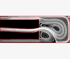
  $50$ (see figure 3b–e). In figure 3(a–e) we observe that the vortical flow region is surrounded by streamlines that trace a path from the inlet to the outlet without recirculating. We refer to this surrounding region as the ‘racetrack’ region in the discussion below. As the Reynolds number increases, in addition to the size of the vortical region increasing, the speed of the racetrack also increases.

Figure 3. Washout time for initial shape. Different symbols represent different Reynolds numbers with associated streamlines shown in (a–e):  $(a)$
$(a)$  $Re = 10$; $(b)$
$(b)$  $Re = 20$; $(c)$
$(c)$  $Re = 30$; $(d)$
$(d)$  $Re = 40$; $(e)$
$(e)$  $Re = 50$; $(f)$ washout time.
In figure 3(f) we plot washout time as a function of the Schmidt number  $Sc$ for five different vales of $Re$. The dimensionless washout time, $T_{90}$, is defined in (2.8). In many biomedical applications, properties of the fluid such as its viscosity and density are fixed. Additionally, the size of the device is likely constrained by physical anatomy, and hence we consider the length scale $a$ to be fixed. Thus, varying the Reynolds number corresponds to changing the inflow rate characterised by $U$. In (2.1b), we non-dimensionalise time on the advection time scale $a/U$, so that the dimensional washout time $T_{90}^{\star }=aT_{90}/U$. In figure 3(f) we present $T_{90}^{\star }$ normalised with respect to the fixed time scale for viscous diffusion of momentum, $a^2/\nu$; this corresponds to $T_{90}^{\star }\mu /(\rho a^2)=T_{90}/Re$.
For  $Sc = 1$, corresponding to a balance between momentum and tracer diffusivities, washout time decreases monotonically with Reynolds number, i.e. the faster the flow (characterised by larger $Re$), the quicker the washout. This can be seen by looking at the symbols on the far left of figure 3(f). In this regime, the tracer diffusivity is sufficiently high that the tracer can diffuse out of the vortex region making its way onto the racetrack. As the speed of the racetrack increases with $Re$, the washout time monotonically decreases with increasing $Re$. As $Sc$ increases – and tracer diffusivity decreases with respect to momentum diffusivity – the vortex-trapping effect becomes more significant, and hence the fastest flow (characterised by $Re$) no longer provides the quickest washout. Since the proportion of the cavity domain occupied by a vortex also increases with $Re$, for $Sc=5$ we in fact see a reversal in the ordering of washout times as $Re$ increases from $20$ to $50$. This is indicated by the lines crossing in figure 3(f) between $Sc = 1$ and $Sc = 5$. Nevertheless, all these washout times beat the washout time for $Re=10$, as although the vortex trapping effect at this Reynolds and Schmidt number is minimal due to small vortex size, the speed of the racetrack for this Reynolds number is comparatively slow, particularly near the rear wall of the cavity. The washout time ordering with Reynolds number remains the same for $Sc = 10$ as for $Sc = 5$. As $Sc$ increases further, however, and the tracer diffusivity is smaller still compared to momentum diffusivity, tracer trapping within the large central vortex – and even the smaller vortex near the exit of the inflow channel – is now so pronounced that for $Re=40$ and $Re = 50$, which have comparatively faster racetrack speeds than the lower Reynolds numbers, washout is slower, as these flow fields also contain the largest central vortices.
3.2. Washout time after vortex optimisation
In figure 4(a) we plot the objective (2.12) – normalised with respect to the objective value at iteration zero – as a function of iteration number. At each value of  $Re$ considered, we observe a broadly monotonic decrease in the objective as a function of iteration number. The optimisation for $Re = 20$ and $Re = 30$ terminates after only 21 and 50 iterations, respectively, caused by the flow problem switching solution branches, and we explain this behaviour in more detail in § 3.3. We see that for $Re = 10$, $Re = 40$ and $Re = 50$ the iterative process continues until the objective curve flattens. In figure 4(b), we consider the relative washout time for $Sc = 5$, defined as the dimensionless washout time (given by (2.8)) normalised with respect to the dimensionless washout time at iteration zero. We plot this relative washout time as a function of iteration number. For $Re = 20$ and $Re = 30$ washout time decreases monotonically with iteration number, correlating with the objective. For $Re = 10$, $Re = 40$ and $Re = 50$, although the behaviour is not strictly monotonic, the washout time has reduced to approximately $90\,\%$ of the initial value by iteration 200. Important to consider is that figure 4(b) only indicates relative improvement of washout time for each value of $Re$, and not a comparison of washout time for different Reynolds numbers. We also note that the washout time in figure 4(b) is only for a single Schmidt number – $Sc = 5$ – and that correlation between objective and washout may improve with increasing $Sc$, although the long washout times with increasing Schmidt number render this comparison a computationally prohibitive task. We quantify the correlation between objective function and washout time in figure 4(c) by plotting these metrics against each other (normalised to zero mean and unit standard deviation for each value of $Re$). We observe that the data follow a roughly linear trend with correlation coefficients $0.9245, 0.9786, 0.8449, 0.925, 0.9291$ for $Re\in \{10, 20, 30, 40, 50\}$.

Figure 4. (a,b) Objective value and washout time ( $Sc = 5$) as a function of iteration number. (c) Normalised (to zero mean and unit standard deviation) objective value and washout and their correlation. The correlation is $0.9245, 0.9786, 0.8449, 0.925, 0.9291$ for $Re\in \{10, 20, 30, 40, 50\}$. $(a)$ Objective function (relative). $(b)$ Washout time (relative). $(c)$ Correlation.
In figure 5(a–e) we show the channel shapes and associated streamlines after the optimisation routine. We emphasise that the optimised channel shape is different for each  $Re$ considered. For Reynolds numbers $Re \in [20,50]$ the optimised inflow channel is now curved, modifying the flow structure observed in the cavity region and decreasing the size of the central vortex. For $Re = 10$ domain symmetry – and hence flow symmetry – has been broken, resulting in slightly reduced vortices near the channel entrance and a faster velocity near the back of the cavity compared to the initial shape (compare figure 5a with figure 3a). It is also worth noting the appearance of a small triangular indent in the bottom outflow of the optimised shapes for $Re = 40$ and $Re = 50$. This is purely an artefact of the discretisation; although this feature plays a role in decreasing the objective function, likely due to singularities in $\boldsymbol {\nabla }\boldsymbol {u}$ at the outflow corners, its influence on $T_{90}$ is negligible. We confirmed that the difference between $T_{90}$ for $Re = 50$ with and without this sharp geometric feature is only of the order of $10^{-5}$. To compare the washout times for the optimised shapes to the washout times for the initial shapes, in figure 5(f) we plot $T_{90}/Re$ as a function of $Sc$ for the final channel geometries and flow patterns produced by the optimisation routine for each value of $Re$. For each $Re$, the corresponding washout times in figure 5(f) have been reduced compared to the washout times for the initial shape at each value of $Sc$ (the washout times for the initial shapes are reproduced from figure 3 in grey). As with the initial shapes, crossings of the lines occur as tracer diffusion decreases, corresponding to the increasing significance – and competing effects – of flow structure and flow speed. Important to observe is that the difference between washout times for the initial and final shapes for a given Reynolds number increases with increasing Schmidt number. This is to be expected: as $Sc$ increases (diffusion decreases) vortex size becomes increasingly significant.

Figure 5. Washout times for final shapes after optimisation. Different symbols represent different Reynolds numbers with associated streamlines shown in (a–e). Red filled symbols correspond to values for optimised geometries, while pale grey symbols correspond to values for initial shapes:  $(a)$
$(a)$  $Re = 10$; $(b)$
$(b)$  $Re = 20$; $(c)$
$(c)$  $Re = 30$; $(d)$
$(d)$  $Re = 40$; $(e)$
$(e)$  $Re = 50$; $(f)$ washout time.
3.3. The effect of multiple solutions
At each iteration of the shape optimisation algorithm described in § 2.4.2 there is an associated channel geometry  $\varOmega _{{t}}^{(k)}$ and velocity and pressure solution $(\boldsymbol {u},p)^{(k)}$. For critical Reynolds number $Re_{{c}}$, if $Re < Re_{{c}}$, then $(\boldsymbol {u},p)^{(k)}$ is unique and stable, whereas if $Re > Re_{{c}}$, then $(\boldsymbol {u},p)^{(k)}$ is one of three possible solutions, two of which are stable, and therefore physically relevant, and one of which is unstable.
For example, for  $\varOmega _{{t}}^{(0)}$, there is a pitchfork bifurcation – displayed in blue in figure 6 – and $Re_{{c}} \approx 12$. For the initial solve with $\varOmega _{{t}}^{(0)}$ when $Re > Re_{{c}}$, we select one of the mirror asymmetric solution branches using the numerical method described at the end of § 2.4.1 and used in Williams et al. (Reference Williams, Castrejon-Pita, Turney, Farrell, Tavener, Moulton and Waters2020). Without loss of generality, we select the solution on the upper branch, as indicated for $Re = 20$ in figure 6 by the blue circle, where we have defined the bifurcation functional as the flux difference between the lower and upper outflows, i.e.
 \begin{equation} \Delta Q = \int_{\varGamma_{{out,l}}} \boldsymbol{u}\boldsymbol{\cdot}\boldsymbol{n}\,\mathrm{d}{s} - \int_{\varGamma_{{out,u}}} \boldsymbol{u}\boldsymbol{\cdot}\boldsymbol{n}\,\mathrm{d}{s}, \end{equation}
where  $\boldsymbol {n} = (-1,0)^\top$ is the outward unit normal vector to $\varGamma _{{out,l}}$ and $\varGamma _{{out,u}}$.

Figure 6. Bifurcation diagrams for  $Re = 20$ at shape iterations $0$,
$0$,  $11$ and $21$. Dashed lines indicate unstable solutions and solid lines stable (physically attainable) ones. The coloured circles indicate the relevant solution during optimisation. The three black symbols indicate the three possible solutions at $Re = 20$ and iteration $21$, with corresponding streamlines presented in (b–d): $(a)$
$(a)$  $Re = 20$ optimisation; $(b)$ Solution 1; $(c)$ Solution 2; $(d)$ Solution 3.
With each shape iteration, the bifurcation structure, and hence the value of  $Re_{{c}}$, changes. If the domain deforms asymmetrically the once perfect pitchfork solution structure becomes a broken pitchfork, as demonstrated by the yellow and red lines in figure 6, where $Re_{{c}}$ which characterises the transition point from one to three solutions is the location of the detached limit point.
This insight allows us to understand the branch switching that causes the early termination of the  $Re = 20$ and $Re = 30$ optimisations (red and yellow lines in figure 4a, respectively). In figure 6(a) we plot the broken pitchfork bifurcation diagrams associated with $\varOmega _{{t}}^{(11)}$ and $\varOmega _{{t}}^{(21)}$ in yellow and red, respectively, with corresponding coloured circles denoting the solutions $(\boldsymbol {u},p)^{(11)}$ and $(\boldsymbol {u},p)^{(21)}$ at $Re=20$ and with solid and dashed lines indicating stable and unstable solution branches respectively. The black triangle, cross and square on the red bifurcation diagram associated with $\varOmega _{{t}}^{(21)}$ denote the three possible solutions at $Re=20$, and their corresponding streamlines are drawn in figure 6(b–d). As iteration number increases from $0$ to $21$,
$21$,  $Re_{{c}}$ increases and approaches $Re = 20$. Iteration $22$ then produces a candidate channel shape with $Re_{{c}} > 20$, and hence only a single solution (on the lower stable branch) exists at $Re = 20$. At this stage the Navier–Stokes solver diverges, as the chosen initial guess – Solution $1$ in figure 6 – is far away from the solution associated with the lower asymmetric branch, and hence is a poor initial guess for the Newton solver.
Of interest to note is that starting the optimisation routine with  $\varOmega _{{t}}^{(21)}$ and the solution for $(\boldsymbol {u},p)^{(21)}$ given by the lower stable branch (Solution 3 in figure 6) instead of the upper stable branch (Solution 1) results in a channel shape similar to that in figure 6(b–d), but flipped with respect to the $x$-axis of the domain. Notably, after several iterations of the optimisation routine the broken and unbroken branches of the pitchfork collide and switch stability – an example of a cusp catastrophe – so we are again on the stable, broken branch of the bifurcation diagram. After several more iterations, a candidate shape with $Re_{{c}} > 20$ is proposed by the optimisation algorithm, and the Navier–Stokes solver diverges again.
Of the five Reynolds numbers we explored, the branch-switching behaviour during the initial optimisation run occurs in only  $Re = 20$ and $Re = 30$ at iterations $21$ and $50$, respectively (see figure 4). For higher Reynolds numbers – e.g. $Re=50$ – the bifurcation diagram never evolves to the stage where $Re_{{c}} > 50$, as would be required to observe the phenomenon described in this section.
Computing bifurcation diagrams for the optimised channel shape highlights an important point: although the optimised flow solution is stable, for some Reynolds numbers it is not the solution one would find by increasing the flow rate in physical practice (or by numerical Reynolds number continuation in computation). To obtain the optimal flow field associated with the optimal shape in reality, techniques such as blocking and unblocking an outflow – previously used to obtain flow fields on a desired branch of a pitchfork bifurcation in experiment (Williams et al. Reference Williams, Castrejon-Pita, Turney, Farrell, Tavener, Moulton and Waters2020) – may be required.
4. Summary and discussion
Many biomedical procedures require efficient clearance of debris, whether to improve visualisation in endoscopic surgeries, or to reduce accumulation of undesirable biological agents in a stented artery or ureter. Debris clearance typically relies on fluid flow – an injected saline solution, contrast agent or blood circulation – and debris aggregation sites can arise as a result of recirculation zones in the fluid. Modelling debris dynamics as the advection and diffusion of a passive tracer, the time required for the tracer to escape a region of closed streamlines depends nonlinearly on the velocity, diffusive properties of the debris and vortex size (Rhines & Young Reference Rhines and Young1983). This motivated the hypothesis that underpins the work in this article: for fixed flow speed and debris characteristics, a reduction in vortex size will promote more efficient debris clearance.
In this paper we considered flow in a 2-D Cartesian geometry, consisting of a rectangular cavity and inlet and outlet channels, and used shape optimisation to determine channel geometries that reduce the presence of vortices. We characterised recirculation zones via  $\det (\boldsymbol {\nabla }\boldsymbol {u})>0$ – i.e. locally circular or spiral streamlines – thereby choosing the objective for our optimisation to be a smoothed form of $\max (0, \det \boldsymbol {\nabla }\boldsymbol {u})$ integrated over the cavity domain (Kasumba & Kunisch Reference Kasumba and Kunisch2012). We determined the relationship between washout time and the objective by solving an advection–diffusion equation for the motion of a passive tracer in both the initial and the optimised flow fields and calculating the resulting washout time. We used $T_{90}$ as the metric characterising washout time, corresponding to the time taken for 90 % of the tracer to exit the domain. We note here that alternatives to $T_{90}$ for the washout metric can be found in the literature: for example, Min et al. (Reference Min, Fischer and Pearlstein2020) track the location and magnitude of the peak of the remaining concentration. A comparison of washout metrics in relation to our objective function would be an interesting future study, but here we chose to restrict attention to $T_{90}$ as this is a commonly used standard measure of washout efficiency.
We first solved for washout time in the initial uniform channel geometry for Reynolds numbers  $Re = 10$, $20$,
$20$,  $30$,
$30$,  $40$ and $50$ and confirmed that washout time depends non-trivially on Reynolds number, flow structure and the diffusion coefficient associated with the passive tracer. When the Schmidt number $Sc = 1$ – i.e. when tracer motion is governed by a balance of momentum diffusivity of the fluid and diffusivity of the concentration – washout time decreases monotonically with increasing Reynolds number. However, for decreased tracer diffusivity, we found that the case of fastest flow ( $Re = 50$) in fact provided the slowest washout time. This seemingly counterintuitive result is easily explained by the fact that the fastest flow also creates the largest vortex, and in an advection-dominated regime vortex size has a dominant impact on washout time.
Running the optimisation algorithm for each of the five Reynolds numbers, we computed the optimal shape and found that washout time is indeed lower in the optimised geometries than in the initial geometries in each case. This partially confirmed the hypothesis that our objective serves as a proxy for washout time. To explore the correlation more thoroughly, we computed washout time for several geometries (and corresponding flow fields) along the optimisation pathway. With  $Re = 20$ and $Re = 30$, washout time decreases monotonically with each shape iteration. For $Re = 10$, $40$ and $50$, washout time is not monotonic with iteration number in the optimisation algorithm, although after $200$ iterations the washout time is reduced to approximately $90\,\%$ of its initial value. This strong, if imperfect, correlation suggests that minimising washout may be well accomplished via a proxy objective measuring the size of vortical structures, a choice that creates significant computational advantage. This reflects the intuitive notion that if tracer transport is not diffusion dominated, tracer can remain ‘stuck’ in vortices for long periods of time, and thus reducing vortical structures can significantly reduce washout time. By construction, $Sc$ does not appear in the optimisation algorithm, but the connection between vortex size and washout suggests that the optimal shape for a given $Re$ will not vary significantly with varying $Sc$, at least in the advection-dominated regime. The connection between washout reduction and the size of vortical structures is less strong in the high-diffusion regime; here maximising flow in the non-vortical ‘racetrack’ regions may be more important than minimising the size of vortices, and a different proxy metric may be more suitable. However, such a regime is less interesting from an optimisation point of view, as it is characterised by very low washout times in any case.
Also of note on the computational side is the fact that, for two of the Reynolds numbers ( $Re = 20$ and $Re = 30$), solution branch switching occurred during the optimisation routine. This feature was shown to occur as an artefact of the evolving broken pitchfork bifurcation structure for the flow problem during the evolution of the channel shape following the optimisation pathway. Such a feature may naturally arise in an optimisation scheme involving multi-solution flow fields, and highlights an important point, particularly when translating to a clinical or industrial setting: the flow field associated with a computed optimal shape may not be the only stable solution, so care may be needed in physically realising the desired optimal flow.
We also explored the washout time corresponding to the optimised channel shapes as a function of the diffusion of the passive tracer, captured by the Schmidt number  $Sc$. As was observed in the base geometry, when plotting washout time against $Sc$ across the set of Reynolds numbers, numerous crossings of the lines are observed. This further underscores the complex relation between washout time, flow speed, vortices and diffusivity. Of course, from a device design point of view, the key question is what shape should the inflow and outflow channels be? Here, in lieu of a single answer, our analysis provides several points of insight: we have shown that the optimal shape is somewhat dependent on the Reynolds number, and the optimal Reynolds number is dependent on the tracer (debris) diffusivity. The diffusivity may not be well known, but we see the importance of a good estimate. In terms of Reynolds number, in practice this can be controlled by changing the upstream driving pressure or fluid properties, in which case figure 5 (or its equivalent in a different geometry) enables us to determine the best combination of shape and Reynolds number. A natural extension would be to optimise for both the Reynolds number and the shape simultaneously. However, in addition to non-trivial extensions of the Fireshape library being necessary for such a combined optimisation, we also expect more difficulties navigating the multiple solution branches if the Reynolds number changes during the optimisation. For these reasons, we do not explore this combined optimisation at this stage.
Even in the absence of a global optimal shape, figure 5 shows a clear qualitative trend that curving the jet of fluid via bending the inlet channel leads to a decrease in the size of vortical structures, and we anticipate that this qualitative finding could carry over to more complex (and possibly 3-D) domain geometries. To test this idea, in figure 7 we have run the optimisation algorithm on a set of three distinct geometries: in figure 7(a,d) we replace the square domain with a smooth curved boundary; in figure 7(b,e) we replace the back edge with an inwardly curved boundary; and in figure 7(c,e) we break the symmetry of the domain through the addition of a circular bulge in the corner. Here, figure 7(a–c) shows the flow pattern and computed  $T_{90}$ for the straight inlet/outlet channels, while figure 7(d–f) shows the optimised shape and corresponding $T_{90}$. For each domain, the total cavity area was preserved, allowing direct comparison of the washout times. Unsurprisingly, the smooth domain in figure 7(a,d) exhibits a much faster washout than the domain in figure 7(c,f), in which debris remains stuck in the small vortex in the additional ‘mini-cavity’. Nevertheless, in all cases we observe a significant reduction in washout time. Perhaps more importantly, the optimised shape for each of the domains is qualitatively very similar, following the same trend of curving the tip of the inlet channel as was found in figure 5. While this is clearly not exhaustive in terms of possible geometric features, it does demonstrate a robustness to the framework and reinforces a design principle that curving the fluid can minimise the size of vortical structures and thus reduce the recirculation of debris.

Figure 7. Optimisation on different geometries: (a–c) the flow pattern and computed  $T_{90}$ before optimisation; (d–f) the same after optimisation. All computations are for $Re = 20$ and $Sc = 20$: $(a)$
$(a)$  $T_{90} = 1449.3$; $(b)$
$(b)$  $T_{90} = 1624.2$; $(c)$
$(c)$  $T_{90} = 2297.4$; $(d)$
$(d)$  $T_{90} = 896.0$; $(e)$
$(e)$  $T_{90} = 1028.9$; $(f)$
$(f)$  $T_{90} = 1815.2$.
An obvious extension to the study reported in this manuscript is to consider 3-D – rather than 2-D – geometries representative of real medical devices. However, a salient factor to consider is computational cost: solving shape optimisation problems involves many ( ${\sim }200$) state and adjoint equation solves. In two dimensions this is possible on a standard workstation, but the computational cost is several orders of magnitude larger in three dimensions. For this reason we focused on a 2-D case in this study, but are cognizant of the significance of the extension to three dimensions. We note that the choice of vortex metric is more open-ended in three dimensions, and a thorough comparison of results using different available metrics remains necessary future work (Jeong & Hussain Reference Jeong and Hussain1995; Haller Reference Haller2005).
Finally, we observe that in the optimisation scheme, the choice of which boundaries are fixed and which are free is important. In our set-up, we fixed the walls at the front of the scope, thereby preventing the inflow channel from flaring or tapering as it enters the cavity. Relaxing this restriction potentially introduces competing effects: a flared tip geometry may reduce the size of vortices, but it also reduces the flow speed of the open streamlines, or ‘racetrack’, as described in § 3.1. For high  $Sc$ (tracer with low diffusivity), debris can get stuck in areas of slow velocity, inducing longer washout times, even though the presence of vortices has been reduced. In this instance, an alternative objective that promotes fast velocity in non-vortex regions – the racetrack – might be suitable, e.g. one could subtract a term from the objective of the form $\int _{\varOmega _{{c}}}|\boldsymbol {u}|\mathcal {H}(-\det \boldsymbol {\nabla }\boldsymbol {u})\,\textrm {d}\varOmega _{{c}}$. However, numerical complexities arise with determining a smoothed version of the indicator function $\mathcal {H}$, and further work is required to implement such a modified metric in practice.
Code availability
For reproducibility we have archived the code and the exact software versions used to produce the results in this paper on Zenodo (Zenodo 2020).
Supplementary movies
Supplementary movies are available at https://doi.org/10.1017/jfm.2020.1119.
Acknowledgements
This publication is based on work supported (or partially supported) by the EPSRC Doctoral Prize Scheme (EP/R513295/1). The authors would like to acknowledge the support of Boston Scientific Corporation. The authors are grateful for discussions with P. Farrell and S. Tavener on using defcon to compute the bifurcation diagrams.
Declaration of interests
The authors report no conflict of interest.


