


1. Measurements on a Wedge-Shaped Glacier Terminus
Temperate glaciers tend to end on land in snouts that are like ramps; their thickness decreases continuously to zero. Detailed measurements of movement are rare and this note concentrates on a set made by Reference GlenGlen (1961) in 1958 and 1959 on Austerdalsbreen, an outflow glacier from the Josterdalsbre ice cap, western Norway. The measurements extended over the last 224 m of the glacier and our purpose here is to find a consistent model to explain them, using the Glen flow law. Glen found, remarkably, that even in the last stake interval on the ice, over a distance 5–21 m from the actual end of the ice, there was still a compressive strain rate of 0.064 a−1. There was a gap a few centimetres wide over almost all the edge (probably melted by heat from the rock below), and where such a gap persisted under the ice it could not be compressing longitudinally. Nevertheless, strain was occurring; the ice was not dead, nor was it being pushed forward as a rigid mass for more than a few metres from the ice edge. When the author revisited the site in 1963 the glacier had retreated, exposing more bedrock. The long profile of the bedrock the ice had been occupying in 1958 and 1959 was surveyed for 240 m (Reference NyeNye, 1970), and therefore the ice thickness for the line of the measurements was known.
Figure 1 shows the measured heights H of points on the top surface of the ice, together with the best straight line passing through the origin. The profile is very close to a straight line, and in fact it is notably closer to a straight line than is the measured profile of the rock bed (not shown). The average slope of the top surface is 0.2748, compared with the average slope of the rock bed of ∼0.095. As a model consider ice, of linearly varying thickness h(x), measured normal to the surface, flowing from left to right down a plane bed of uniform small slope β (Fig. 2). Although the ice is wedge-shaped we calculate the velocity distribution within the ice as if the top and bottom surfaces were locally parallel. This is, of course, an approximation. The origin is the end of the glacier with the x axis parallel to the top surface and pointing down the slope. Thus the glacier occupies the negative part of the x axis. The y axis points upwards normal to the surface. The shear stress component τxy , which is the driving stress for the shear strain rate, is governed predominantly by the slope of the top surface rather than the bottom. It is given by τxy = −ρgxy where gx is the component of gravity.

Fig. 1. The measured heights of points on the upper surface of the ice plotted against x to give a profile, and a straight line of best fit.

Fig. 2. The coordinate system for the model. The angles shown are those measured.
We write the Glen flow law in the form
where
![]() is the effective strain rate and τ is the effective shear stress (Reference NyeNye, 1957).
is the effective strain rate and τ is the effective shear stress (Reference NyeNye, 1957).
2. Two Flow Models
One might think, perhaps, that a possible model to explain the velocity would simply combine motion from laminar flow within the ice with basal sliding. It would lead to an expression for the velocity, averaged over the thickness, of the form u(x) = u d(x) + u b(x) with the first term u d(x) coming from the Glen flow law for simple shear and the second from a suitable law of basal sliding.
The velocities measured at the stakes on the upper surface are shown in Figure 3 and they can be reasonably well fitted by the straight line shown. However, without going into details, the fact is that no fit using laminar flow added to basal sliding can be made without assuming quite implausible values for the constants in the two laws. The orders of magnitude given by such equations are clearly wrong and the linear change of velocity is also a problem, because α is constant and h is varying linearly, so the velocity should vary as h 4, say, instead of h (Reference NyeNye, 1952). However, it can be deduced at once that, on the reasonable assumption that the profile of the surface continues to be a straight line, the effect of the nearly uniform compression rate would be to steepen it by 1.5° a−1, that is, by 9.5% of its angle, a considerable annual change. How the profile really changed in the years after the measurements is not known.

Fig. 3. The measured horizontal component of velocity u is plotted against x and a straight line of best fit is shown.
This situation suggests that a different model, namely that described in Nye (1959) which uses the Glen flow law but not laminar flow, may be more appropriate. It explicitly contains a uniform longitudinal rate of compression r 0, which we can take from the observations of velocity, and it considers the nonlinear interaction of this longitudinal strain rate with the shearing of one layer over another. It assumes plane strain with no movement normal to the vertical xy plane.
The velocity has components u and v. A is given by Eqn (1). Let the unit of time be
![]() and let the unit of stress τ
0 be given by r
0 = (τ
0/A)
n
. Let the unit of length be l
0 = τ
0/ρgx
and the unit of velocity v
0 = r
0
l
0. The solution is then written in terms of non-dimensional variables defined as
and let the unit of stress τ
0 be given by r
0 = (τ
0/A)
n
. Let the unit of length be l
0 = τ
0/ρgx
and the unit of velocity v
0 = r
0
l
0. The solution is then written in terms of non-dimensional variables defined as
τ is the ‘effective shear stress’ of Eqn (1). Its non-dimensional form T is an implicit function of Y through
There are two solutions for the velocity components, U and V, and both are expressed in terms of T, which may be regarded as a parameter. Thus
We choose the lower sign because this gives longitudinal compression with U decreasing with X. Since Y bed is negative it gives V positive within the ice. In view of Eqn (3), Eqn (5) is just the simple linear relation
The plot of U as a function of Y in Figure 4 requires explanation. It omits from Eqn (4) the term linear in X, and is thus a plot of U + X against Y. In spite of first appearances the plot applies perfectly well at all X, even near the end where the ice thickness is tapering down to zero. For example, suppose X is small and negative. Y bed will be small and negative so that only the topmost part of the plot is relevant, where the whole curve is nearly vertical. There is only a small difference in forward velocity between the top and bottom of the ice, so that it is moving almost as a rigid wedge. Or consider a large negative X value. Y bed is large and negative and the whole of the plot is now within the ice, so that there is a considerable difference in velocity between top and bottom. The solution includes pure laminar flow r 0 =0 as a limit, but this is not evident from Eqns (4) and (5) because we have chosen to use r 0 to define our unit of strain rate. The proof is given in Reference NyeNye (1957).
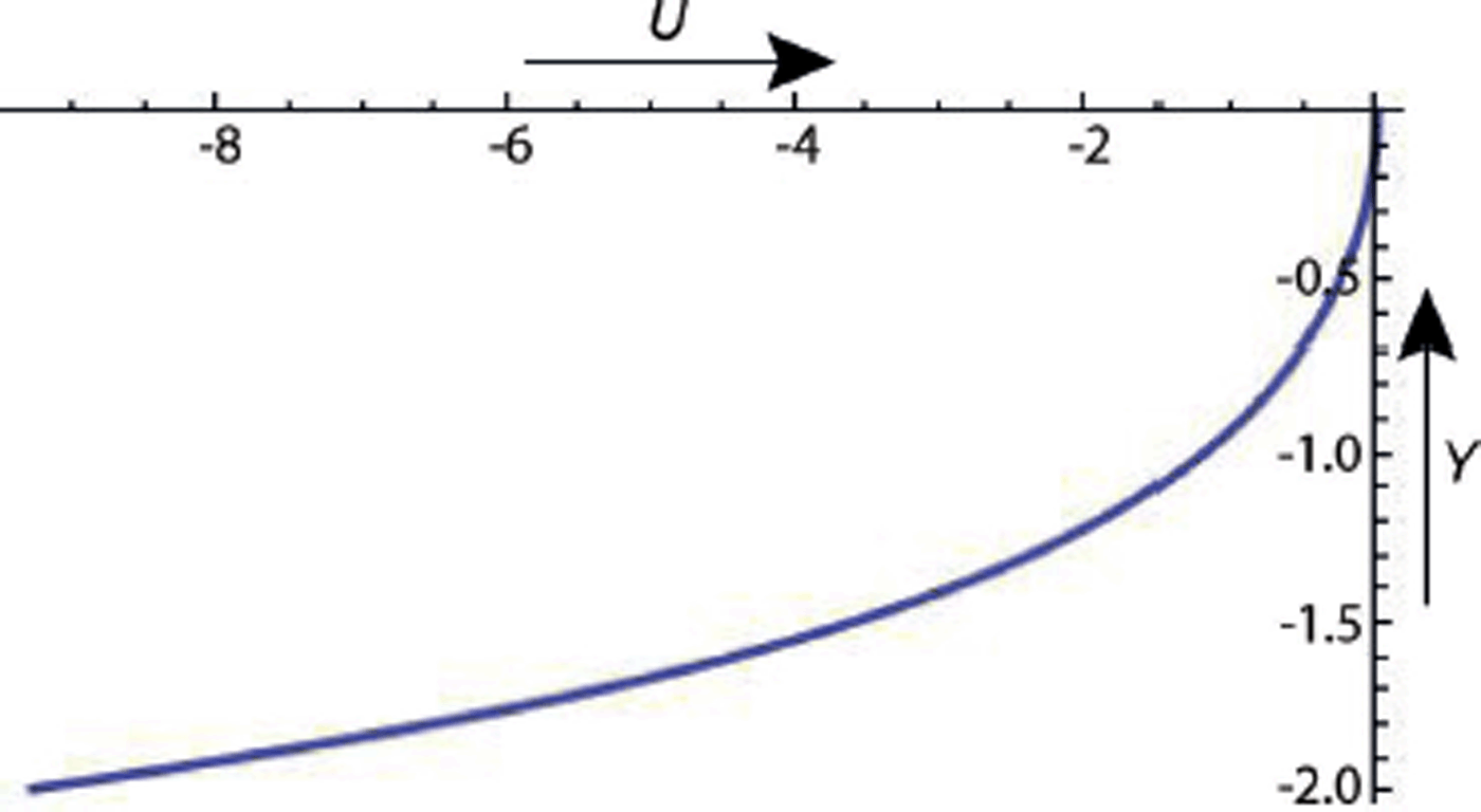
Fig. 4. Theoretical X component of velocity U plotted against Y for n = 3.07.
We have seen that the velocity u as measured by Glen can be well fitted by a constant plus a linear part. The linear part has been used to supply the value of r 0 in the theoretical solution. If we take as possible numerical values n = 3.07 with A = 4.89 ×10⁷ SI units, the measured r 0 corresponds to a longitudinal compressive stress component of 8.3 × 10⁴ Pa, which is very plausible for ice at the melting point. This is in marked contrast to the very different and hence quite implausible values that would be demanded by a pure laminar flow hypothesis, as we have noted above. A comparison of the straight line and the points in Figure 3 shows that the measured velocity is slightly higher than the straight-line values at the top end of the range. This effect is probably explained by the fact that the left-hand half of the rock profile is a roche moutonnée and so is steeper. A quadratic term might be added, but the complication is hardly worthwhile.
The velocity at the end of the glacier (the origin), measured as 8.13 m a−1 by extrapolation of the velocities measured at the stakes, appears in the theory as just an arbitrary constant U 0. Its value cannot be predicted by a theory like this that is solely concerned with deformation within the ice mass. The bed consists of hard rock, so what is needed here is a Weertman-type sliding theory that takes account of the unusually low overburden pressures and the resulting cavitation. This might be difficult in view of the observation that, as the end of the ice is approached, the horizontal component of the velocity consistently decreases even though the pressure must be diminishing. Explaining this decrease is a different kind of problem that can be treated separately and a solution will not be pursued here.
At this point it is instructive to look back at a previous less successful attempt (Reference NyeNye, 1967) to solve the same problem. It made the rather extreme assumption that the ice was behaving like a perfectly plastic material with a sharp yield point (Reference HillHill, 1950) and was in a steady state. But it had the merit of being exact (numerically). The ice slipped over a bed that was horizontal and was virtually a plane and it ended in the shape of a wedge. The computed angle of the wedge was very close to 45°. There was reason to modify the parabolic profile first calculated by Reference OrowanOrowan (1949) which was vertical at the edge. The shape remained the same parabola but translated so that the angle at the edge became 2/π ≃ 36.5°. This parabolic profile then agreed very well with the new exact solution. So far as the fast longitudinal compression observed by Glen was concerned, the conclusion was that although the perfectly plastic model did not show the observed spatial distribution, the orders of magnitude agreed. But one would hardly have expected any very close agreement from an assumption of perfect plasticity.
The approach taken in this note is quite different. It does not mention mass balance, a rate of ablation or a steady state. It simply asks how a wedge-shaped mass of ice would deform and slide when placed on a rough sloping bed. To answer the question it treats the slopes as small, so that the shear stress is mainly due to the slope of the upper surface, and this makes it legitimate to use exact results from a model with parallel faces and a nonlinear, realistic, n ≃ 3 flow law. The fact that the terminus thus modelled was in rapid retreat is irrelevant. It is unfortunate that all the available data have been used up in fitting the constants in the theory, so that no further tests can now be made. They would have involved measuring velocities within the ice.
It is perhaps worth adding that the only application of this solution up to now, apart from the original one in Reference NyeNye (1957), seems to have been to use it to check numerical code for modelling the behaviour of large ice sheets. The bounding cells of such models naturally contain the ice edge, and its position is usually the output of interest. But this is precisely where the models fail. The consequent inconsistency may be dismissed as academic in view of the small size of the cells, but it could be removed completely by taking proper account of the longitudinal compressive strain rate in the way described here. The prospect of this small but worthwhile advance would justify the minimal expense of making similar measurements at other sites.
In summary, the conclusion is that the field measurements on Austerdalsbreen can be explained by a nonlinear model that takes proper account of the nonlinear interaction between the longitudinal and the shear components of the strain-rate tensor.
Acknowledgements
I thank the International Glaciological Society for their help in publishing this note.


