Solving Problems in State Politics Research

The CSPP is designed to take advantage of the tremendous opportunity afforded by research on the American states. State politics are important arenas for democratic contestation; state governments are key actors in public policy; and states are principal laboratories for assessing socioeconomic outcomes of political choices. The states offer leverage across both structures and polities, enabling assessments of variation in behavior and institutions in American governance. They are also connected within a federal system, allowing meaningful analyses of interdependence. The long closely-tracked history of roughly similar cases undergoing national, regional, and local changes over time has made states a premier example of how panel data can be used for description and identification in social science.

To help state research expand and improve, CSPP solves four common problems that otherwise limit achievements in the subfield. First, as a repository for myriad data, it enables ease of use and updating. The vastness of variables on states—from numerous policies and outcomes to related social, political, and economic data—can seem overwhelming rather than advantageous to researchers, instructors, and practitioners. This is particularly the case if the data span different time periods and units of observation, or remain hidden in replication files (or worse, on unconnected personal archives) associated with individual projects. By linking these data, mitigating mistakes in merging, aggregating data by state-year, and updating previously collected data when available, CSPP puts these variables in a unified structure and in commonly used data formats.

A persistent problem with state policy and politics research has been the lack of data availability and access, with researchers frequently reduplicating efforts. The field lags behind some other subfields that have central repositories (e.g., Policy Agendas Project and Correlates of War Project). Fortunately, several scholars have led by example, making their data publicly available (e.g., Walker Reference Walker1969; Gray and Lowery Reference Gray and Lowery1988; Erikson et al. Reference Erikson, Wright, Wright and McIver1993; Berry, Fording, and Hanson Reference Berry, Fording and Hanson1998; Squire Reference Squire2007, Squire Reference Squire2008; Brace and Hall Reference Brace and Hall2009). More recent contributions from generous scholars have exponentially added to the scope of available information (e.g., Boehmke and Skinner Reference Boehmke and Skinner2012; Boehmke et al. Reference Boehmke, Brockway, Desmarais, Harden, LaCombe, Linder and Wallach2020; Caughey and Warshaw Reference Caughey and Warshaw2016, Caughey and Warshaw Reference Caughey and Warshaw2018; Carsey et al. Reference Carsey, Niemi, Berry, Powell and Snyder2008; Klarner Reference Klarner2013a; Shor and McCarty Reference Shor and McCarty2011; Sorens, Muedini, and Ruger Reference Sorens, Muedini and Ruger2008). CSPP would not be conceivable without their important data contributions (which are promoted on the project website). Beyond individual decisions to share data, recent trends such as the open source revolution and expectations of reproducibility have further increased availability. Nongovernmental organizations and universities also have published state-level data (e.g., Open States, Stateminder, National Conference of State Legislators, Ballotpedia, and Council of State Governments). Despite these positive developments, researchers still typically have to cobble together state politics data from scattered, albeit more accessible, sources. That is a central problem we aim to solve.

Social science has also come under fire for cherry picking data to demonstrate relationships. The second large impact of CSPP is to allow researchers not only to select the most relevant policies and outcomes for their analyses, but also to understand the universe of variables from which they are selecting. It is often appropriate to home in on the most closely associated predictors or outcomes of particular policies. CSPP allows the scholarly community to investigate whether those relationships are specific to data choices or part of a broader pattern. For example, a researcher may find that governor partisanship correlates with the relative tax rates paid by Black and White families; CSPP enables a researcher to inspect whether that relationship is part of a pattern across tax policies or racial disparities or simply a singular association, and to assess the durability of that relationship.

Third, the increased emphasis on causal identification in social science has popularized new techniques that require panel data that meets particular assumptions. CSPP allows researchers to assess change over time and variation across states to determine whether they can productively use difference-in-differences, regression discontinuity, fixed effects, quantile regression, or other designs. Researchers may want to study the effects of closely divided legislatures or a particular policy change, for example, but discover that variation is too limited or too closely associated with a broader regional shift. CSPP facilitates searches for instrumental variables, natural experiments, or changes separated from regional or national political dynamics. The comprehensive nature of CSPP’s data facilitates researchers’ ability to match research design to theory, diagnose problems with a given design, and test the robustness of inferences to specification choices.

Finally, the state politics literature remains segregated from the wider interdisciplinary community interested in variation across the United States. In particular, scholars interested in outcomes such as income inequality, public health, educational attainment, and environmental degradation may also be concerned with state-level policies and contextual factors, but are sometimes unaware of the standard variables political scientists use to explain variation. In some cases (e.g., education and health), these research communities are larger than the state politics subfield and may connect political scientists with important outcomes of interest in existing well-financed research efforts. CSPP makes it easier for interdisciplinary researchers to find the data subset they need for topic-specific research, increasing awareness of the importance of political variables in socioeconomic trends. Indeed, we later show that dozens of other criminal justice, education, public health, sociology, and public administration scholars have already taken advantage of CSPP.

The CSPP Database

The CSPP database is able to address those common problems for state researchers because it offers four major advantages: its (1) scale, (2) span, (3) accessibility, and (4) sustainability. First, CSPP is remarkable in its scale. It includes 2,200 variables from across the 50 US states and the District of Columbia pooled from multiple reputable academic, governmental, and nongovernmental sources.Footnote ¹

Table 1 displays the variable categories, number of variables for each category, and example variables included in the database. There are many variables covering economics, government institutions, and health, but fewer variables covering policy areas like social welfare and labor. Although most variables are directly related to policy, many of the variables in each category could also be broader antecedents or consequences of individual policy choices (e.g., institutional and electoral variables, policy liberalism, interest group density, or demographics). The compendium also allows the state politics research community to see where past researchers have focused (e.g., fiscal and drug policy) and where there may still be holes in our collective understanding (e.g., labor and transportation).

Table 1. Variables by category

Beyond these policy, political, socioeconomic, and demographic variables, the CSPP also encompasses two additional data resources. Users can access a dataset containing nearly 7,800 ballot measures attempted across US states from 1902 – 2016. Compiled by the National Conference of State Legislatures (NCSL) (2016), the dataset includes the different kinds of measures pursued (i.e., legislative referendum, initiative, popular referendum, and other), election type (i.e., general, primary, and special), passage rates, and topic areas. By linking the datasets, users can also assess how ballot measures and outcomes are related to other state differences. Researchers can likewise explore or incorporate relevant state network data in their analyses. Assembled by Olson (Reference Olson2019), the state network data consists of state-to-state relational variables including measures of shared borders, trade and travel between states, and similarities along political, socioeconomic, or demographic dimensions. Researchers can assess the network linkages across states (not only state borders, but also many other social ties) to the policy outcomes they study in the CSPP state attribute data.

Most other large-scale state politics datasets are narrower in focus by design. For example, some datasets (e.g., Boehmke et al. Reference Boehmke, Brockway, Desmarais, Harden, LaCombe, Linder and Wallach2020) provide binary variables for policy adoptions but lack variables capturing state institutional features. Other datasets (e.g., Carsey et al. Reference Carsey, Niemi, Berry, Powell and Snyder2008; Klarner Reference Klarner2013d) cover legislative elections or state partisan control, but no variables measuring elite and mass public attitudes. CSPP builds on these datasets by merging them through common unique identifiers (while providing additional IDs such as Federal Information Processing Standards [FIPS] codes) and including an array of additional covariates and policies. We rely on hundreds of data collectors and aggregators, but the website highlights the five largest contributors who were each responsible for providing more than 50 variables. In constructing the dataset, we made a concerted effort to compile both familiar and obscure state policy and politics variables across diverse categories from multiple reputable sources. The resulting dataset and associated software is a comprehensive if not exhaustive outlet for data originators and researchers seeking information on the US states.

The second advantage of CSPP is its time coverage. The database extends from 1900 to 2020. Although, only a few variables extend as far back as 1900 (e.g., total state population), many of the variables span the last four most recent decades. Figure 1 reports the number of variables available by decade. Coverage is at its height in the 21st century, with the fewest variables available in 1900 and monotonically increasing coverage in each decade of the 20th century and then a spike in the 2000s. Analyses using CSPP can take advantage of tremendous temporal variation, but only if the variables needed are available for the full time series. We have the most evidence about recent changes in the states, which means our analyses might not generalize farther back in time. We view this as partially a product of our data compilation but also indicative of data availability in the field. Many contemporary multivariate panel studies may be applicable only in a narrow time frame.

Figure 1. Variable coverage by decade.

Note: The x-axis consists of decades covered by CSPP data. The y-axis is the raw number of variables with values per decade.

Table 2 reports the average number of states available for each variable in each decade. Again, we see widespread coverage in the most recent decades, with nearly all states covered for many variables. Still, several of the variables have a few missing subunits, such as Nebraska, Alaska, Hawaii, and the District of Columbia. Fortunately, limited state coverage is less of a problem for the field and the dataset, though our studies’ findings may not always generalize to all fifty states.

Table 2. Variables by decade

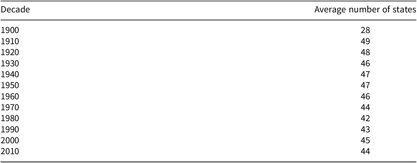
Note: This table displays the coverage of the CSPP data by decade. The second column is calculated as the average number of states, per decade, that have full coverage in the variables.

CSPP’s third asset is its accessibility. Variables are coded at the state-year unit of observation (with notes accounting for aggregation and definition differences).Footnote ² Formatting across the variables is standard, making data management and manipulation easier. Moreover, the database is available in multiple formats, including as a Microsoft Excel file with separate content area sheets, a comma-separated values (CSV) file containing all the variables, and an R package (CSPP; Lucas and McCrain Reference Lucas and McCrain2020). Accompanying the package is a Shiny App web application that allows users to subset, explore, and download CSPP variables and corresponding citations. The R package and associated app also allow users to create visualizations, including maps, time trends, correlation matrices, and network diagrams.Footnote ³ CSPP also comes with a searchable, detailed codebook containing complete variable names, time spans, descriptions, original sources, and notes. The codebook and package allow for easy perusal of variables and original sources.

CSPP’s fourth benefit is the system in place to ensure the database is maintained, updated, and expanded. Both the Institute for Public Policy and Social Research (IPPSR) and Michigan State University (MSU) have committed resources to compensate undergraduate and graduate students to help ensure appropriate data documentation, update existing variables, add new variables, correct errors, and release new versions of the database in a timely manner. In fact, hundreds of additional variables are planned for future releases of the database. Related, CSPP aims to reward the data producers by encouraging users to cite the original source, as well as tracking and publishing statistics on use so that originators can include these metrics in their citation counts. The R package and web app also allow users to easily compile citations for all of the original variables they utilize.

To be sure, such an enterprise is not without risk. Pooling variables from multiple sources can yield missing data or inaccuracies. These data gaps or inconsistencies may result from missing observations in the original source, coding errors made by the primary source, or data transfer mistakes on our end. For instance, if observations are missing for a particular jurisdiction or year in the original source, these observations are also missing in our database. Furthermore, if mistakes were made in creating or coding data by the primary sources, these errors will also be reproduced in our database. Although we have made considerable effort to ensure data quality and integrity during transfers and aggregation, errors are still possible. We encourage users to check the accuracy of the data, relying on the primary sources. We also appeal to researchers to inform us if they uncover any errors. As we are made aware of data inaccuracies, our team corrects the inconsistencies, promptly updates the database, and informs users of the changes via errata in future release versions. The dataset also allows comparison of multiple measures of the same concept, which we often keep for potential robustness checks as inconsistencies are usually due to subtle differences in coding choices.

Current Use of CSPP

Demonstrating the utility of CSPP and how it is already helping solve problems in US state research, CSPP has been cited by 100 papers, articles, and books (after consolidating near duplicates). Nearly all citations were from the last three years and many were not yet published (21 were from dissertations or theses), suggesting that usage is just beginning to take off. We analyzed these citations to determine how CSPP is currently being used by researchers. Most scholars relied on the CSPP for specific variables (90% of citations), while others made general reference to the database. Most analyses using CSPP made causal inference claims (90% of citations) while others used the variables for descriptive work (6%) or general reviews (3%). Despite attempting to make causal inferences, however, most researchers used a standard panel or cross-sectional research design, with only 47% employing fixed-effects, and only a few others using regression discontinuity or other quasi-experimental approaches.

Although most users have yet to fully leverage CSPP for causal research, many are capitalizing on the breadth and span of the database. Exploring regional variation was a common area of investigation (81% of projects conducted some kind of regional analysis), though it was rarely the main focus of research. Similarly, partisan differences and polarization were common topics (probed in 40% of projects), but they were the focus of only 12 projects. The modal project examined a particular policy area, using panel data to investigate public policy choices or effects. Overall, 30 different policy issue topics were covered by researchers (spanning nearly every major issue area). Slightly more studies use public policy as an independent variable (54%) than a dependent variable (49%). The total exceeds 100% because some studies used policy for both (though others used it for neither). Many of the studies utilize CSPP variables for controls. While some of the researchers’ projects extended decades back in time, most investigated contemporary periods, with the average analysis beginning in 1980 and ending in 2013. Underscoring CSPP’s inroads in other disciplines, the database has been used by researchers representing diverse subfields. Although most of the authors citing CSPP are political scientists (63%), sociologists (16%), economists (18%), psychologists, criminal justice scholars, public administration researchers, environmental scientists, and many others have also used CSPP.

To see how data compilation enables multiple analyses, we want to highlight two dissimilar uses of CSPP to study the same topic: the effects of state partisanship on socioeconomic outcomes. Grumbach (Reference Grumbach2018) relies in part on CSPP to examine the polarization of 16 different policy areas across the US states since the 1970s. He finds that the party that controls state government is an increasingly strong predictor of policy outputs in many of the issue areas. Grumbach then shows how that partisan polarization leads to divergent outcomes tied to those policy differences, including incarceration rates and health insurance access. Grumbach’s use of CSPP showcases how researchers can pinpoint the effects of consequential policies driven by state politics, revealing significant externalities for states.

Dynes and Holbein (Reference Dynes and Holbein2020) take a broader approach to state outcomes. They use CSPP data to employ both difference-in-differences and regression discontinuity designs to explore how state government party control influences overall socioeconomic outcomes. Rather than select outcomes most likely to be a result of particular party-linked policies, Dynes and Holbein examine dozens of outcomes to assess partisan differences in fulfilling common policy objectives. They find that Democratic- and Republican-controlled governments perform equally well across these objective output measures. Their approach tempers any generalization of party effects on broad state outcomes. Both articles offer important insights: some outcomes are associated with particular policies enacted by partisan governments (as Grumbach finds), but the broader trajectory of states is not dependent on their partisanship (as Dynes and Holbein show).

Regional and Temporal Variation

CSPP’s data and tools offer opportunities for researchers to find relevant state variables to answer theory-driven questions employing multiple research designs. But users should also be aware of the dual complexities of using US state panel data. On the one hand, many state attributes remain relatively stable over time. On the other, the nation as a whole has experienced some pronounced regional differences and temporal change. Regional analysis is very common in studies citing CSPP and important in understanding the often-limited sources of variation in state politics. Given that CSPP-enabled studies thus far often employ panel data to assess causal claims (sometimes without quasi-experimental methods), it is critical to understand these patterns and the challenges they produce.

To illustrate this common structure of state panel data, we present the distributional characteristics of four commonly used indices in state politics research: policy mood (where higher scores indicate a more liberal citizenry; Enns and Koch Reference Enns and Koch2013), income inequality (a Gini coefficient, where higher measures indicate greater income concentration; Frank Reference Frank2014), policy liberalism (where higher scores point to more liberal policy adoptions; Caughey and Warshaw Reference Caughey and Warshaw2016), and union density within a state (measuring the proportion of non-agricultural workforce represented by a union; Kelly and Witko Reference Kelly and Witko2014). For these illustrations, we categorize states into the four familiar regions: the Northeast (Maine to Pennsylvania), the Midwest (Ohio to Kansas to the Dakotas), the South (states of the confederacy plus Delaware, the District of Columbia, Kentucky, Maryland, Oklahoma, and West Virginia), and the West (the Mountain and Pacific time zones). Other state divisions show similar effects.

Figure 2 displays the density plots for these four variables standardized across each geographic region from 1990 to 2010. For policy liberalism, the results indicate (unsurprisingly) that the Northeast is the most liberal, while the South is the most conservative. There is considerable variation in policy liberalism in the West and Midwest. Policy mood largely mirrors policy liberalism, with the Northeast displaying more progressive citizens than the other regions, but with little variation across the other regions. Union density fluctuates considerably in all regions besides the South, where it is much lower. Lastly, income inequality shows greater variation at the high end in each region, with limited average regional differences.

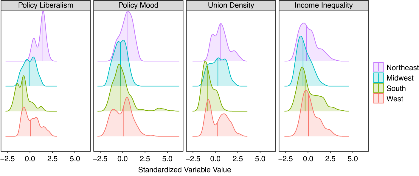
Figure 2. Densities of variables by region.

Note: Each panel is a variable in CSPP data spanning from 1990 to 2010 with sources discussed above. The variables were standardized prior to plotting. The densities of each variable are plotted disaggregated by region, starting from the top: Northeast, Midwest, South, and West.

Further demonstrating regional variation for key attributes, Figure 3 displays the correlations within regions for several commonly used variables.Footnote ⁴ To the previous four variables, we add gross state product per capita (US Department of Commerce Bureau of Economic Analysis, 2012), lower (House) and upper (Senate) chamber polarization (Shor and McCarty Reference Shor and McCarty2011), party control (where 0 is unified Republican control, 0.5 is neither party full control, and 1 is unified Democratic control; Klarner Reference Klarner2013b), policy innovativeness (indicating a state’s willingness to adopt new policies sooner than other states; Boehmke and Skinner Reference Boehmke and Skinner2012), and legislative professionalism (the first dimension scaled from legislator salary and expenditures and session length; Bowen and Greene Reference Bowen and Greene2014).

Figure 3. Variable correlation by region

Note: This figure shows heatmaps of the bivariate correlations of variables of interest, separated by region. Darker colors indicate stronger correlations. Orange shading indicates a positive correlation, while blue shading indicates a negative correlation.

Most analyses look for associations among these variables nationwide, but that could present a misleading picture if there is regional heterogeneity. Policy liberalism, for example, is negatively correlated with income inequality (Gini coefficient) in all regions except the Northeast. Democratic party control is negatively associated with polarization in the South but positively associated with it in other regions. Similarly, union density has a negative correlation with legislative professionalism in the South, but the inverse is true in the other regions. Meanwhile, greater union density in the Midwest is associated with higher polarization, but the opposite holds for other zones. These regional trends reinforce the need to account for potential regional heterogeneity in our investigations.

Most CSPP-enabled panel models also assume that estimated relationships are constant over time. Empirically, however, there is variation in the associations among variables. Figure 4 showcases this using the same variables presented in Figure 3, displaying the changes in these correlations between 1990 and 2010.Footnote ⁵ The results indicate that many of the relationships with inequality are decreasing over time, whereas the associations with party control are increasing over these decades. Likewise, policy innovativeness’ relationship to many of these variables has also waned during this period. Importantly, what is true in one era may not be true in the next.

Figure 4. Difference in correlations across decades.

Note: This figure plots the differences in bivariate correlations between 1990–2000 and 2000–2010. The raw change in the correlation is displayed within each cell. For instance, if the correlation between two variables was 0.8 in 1990–2000 and then 0.3 between 2000 and 2010, the value in that cell would take on −0.5. The decade-level correlations are presented in the Supplementary Appendix. Darker colors indicate larger correlations. Orange shading indicates a positive correlation, while blue shading indicates a negative correlation.

Equally important, panel-based statistical analyses require attention to serial correlation and time trends. Figure 5 illustrates temporal differences by region for the original four variables (i.e., policy liberalism, policy mood, union density, and income inequality).Footnote ⁶ Policy liberalism shows steady change by region, with the Northeast trending leftward, the Midwest and South trending a bit rightward, and little change in the West. Policy mood shows notable volatility, with a national decline followed by an increase with regional dispersion. Union density is declining across regions, with regional differences between the Northeast and South. Income inequality trends are mostly national, with a marked uptick after 2000 and little regional variation. Relating any two of these trends in panel data would need to account for whether the variation was across states or time.

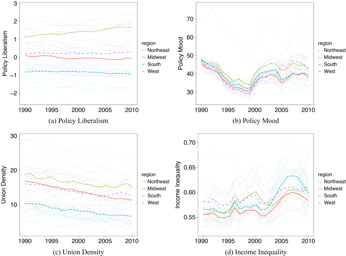
Figure 5. Temporal variation.

Note: Each panel depicts the over-time values of a variable of interest from 1990 to 2010, both with individual lines per state (transparent) and darker lines reflecting the regional mean.

An Application to Public Opinion and Policy Liberalism

To further illustrate the opportunities and challenges of using US state panel data with different regional and temporal patterns, we address a common application: the potential relationship between public opinion and public policy in the American laboratories (see Berry, Fording, and Hanson Reference Berry, Fording and Hanson1998; Berry et al. Reference Berry, Fording, Ringquist, Hanson and Klarner2010; Caughey and Warshaw Reference Caughey and Warshaw2018, Caughey and Warshaw Reference Caughey and Warshaw2016; Enns and Koch Reference Enns and Koch2013; Wright Jr., Erikson, and McIver Reference Wright, Erikson and McIver1987). States with more liberal electorates, such as California, also tend to enact more liberal policies. There are, of course, many (political, institutional, socioeconomic, and demographic) factors that may explain this relationship. And since both state public opinion and policies are relatively stable, we cannot discern from the relationship alone that public opinion leads to policy differences.

Figure 6 reveals the overall liberalism of state policy and public opinion, averaging over the 1990s and 2000s, using the same measures we used above (we explore several alternative measures with similar results in the Supplementary Appendix). The results show largely familiar regional and partisan patterns. But to what extent and how do these quantities covary? Although causal identification is clearly complicated, we can use the panel structure of the data to isolate potential confounding and unobserved sources of variation. There are many potential models that might be used to assess the relationship. For illustrations, we include two classes of models that are common in the state politics literature and take the form of:

(1) $$ \begin{array}{r}{\mathbf{Y}}_{st}={\beta}_{st}+{\mathbf{I}}_{st}+{\mathbf{S}}_{st}+{\gamma}_t+{\epsilon}_s\end{array} $$

and

(2) $$ \begin{array}{r}{\mathbf{Y}}_{st}={\beta}_{st}+{\mathbf{I}}_{st}+{\mathbf{S}}_{st}+{\gamma}_t+{\theta}_s+{\epsilon}_s,\end{array} $$

where $ {\beta}_{st} $ is the independent variable or treatment for a given state s in year t, $ {\mathbf{Y}}_{st} $ is a specific outcome, $ {\mathbf{I}}_{st} $ is a vector of time-varying institutional controls (e.g., legislative professionalism, unified or divided government), $ {\mathbf{S}}_{st} $ is a vector of time-varying socioeconomic and demographic controls (e.g., population, income inequality, and gross state product per capita), $ {\gamma}_t $ is a year fixed-effect to absorb common year-specific shocks (e.g., recessions and election years), and $ {\epsilon}_s $ are state-clustered standard errors. The difference in these two specifications comes through the inclusion of time-invariant state controls or a state fixed-effect $ {\theta}_s $ . The former case typically includes a regional dummy, such as a control for the state being in the South. The latter case, with state fixed-effects, absorbs all unobserved time-invariant traits of the state, such as fixed regional or cultural variation, and produces an estimate for β within the state.Footnote ⁷

Figure 6. Maps of policy liberalism and state policy mood.

Note: Darker shades represent higher values of each variable. Values are averages per state from 1990 to 2010.

We run three separate classes of models using variations of these two equations. The first set of models includes only year fixed-effects, the second includes year and region fixed-effects, and the final includes year and state fixed-effects. The institutional set of controls consists of: legislative professionalism (Bowen and Greene Reference Bowen and Greene2014), the distance between party medians in the upper and lower chambers (Shor and McCarty Reference Shor and McCarty2011), union density (Kelly and Witko Reference Kelly and Witko2014), and party control of state government (Klarner Reference Klarner2013b). The demographic and socio-economic controls consist of: logged population total from the Census, the Gini coefficient (Frank Reference Frank2014), gross state product per capita (Cummins and Weiss Reference Cummins, Weiss and Dionne2013), and state consumer price index (Berry, Fording, and Hanson Reference Berry, Fording and Hanson2000). We lag all controls to account for concerns surrounding post-treatment bias (Montgomery, Nyhan, and Torres Reference Montgomery, Nyhan and Torres2018), but that does not imply that the version with the most controls is necessarily preferable. Instead, the application is designed to show the complexities and impact of model specification. For all analyses the independent variable of interest is state policy mood (Enns and Koch Reference Enns and Koch2013), and the outcome is policy liberalism (Caughey and Warshaw Reference Caughey and Warshaw2016).

In the pooled models with only year fixed-effects, the comparison produced is across states, assessing, for instance, how California compares to Montana. Introducing regional fixed-effects adjusts the comparison, creating a region-specific intercept and holding fixed anything unobserved that does not change within region. Finally, in the state fixed-effects specification, the variation is produced within states. Substantively what this means is that if there is minimal variation in the outcome within one state overtime, most of the effect of β will be absorbed by the state fixed-effect. For each specification we run the models without controls, with only institutional controls, and with institutional and socioeconomic controls.

Figure 7 plots the coefficient estimate for policy mood (β).Footnote ⁸ This figure directly compares the estimated coefficients from these model specifications, including regional time trends and lagged independent variables. All models are presented in full in the Supplementary Appendix. As is clear in this figure, there is substantial attenuation in the size of the coefficient once accounting for observed and unobserved socioeconomic and institutional characteristics of states.Footnote ⁹ Once all time-invariant state characteristics (observed and unobserved) are isolated out with the inclusion of state fixed-effects, the coefficient estimate is near zero (though some control variables may be partial consequences of citizen ideology). This finding echoes Caughey and Warshaw (Reference Caughey and Warshaw2018), who find that increasing specification stringency lowers estimated effect sizes. This is not to suggest that the most constrained model is the correct one, only to acknowledge the common inferential difficulties.

Figure 7. Estimated coefficients by different model specifications.

Note: Models are presented in full in the Supplementary Appendix. The outcome for each model is policy liberalism, and the plotted coefficient is state policy mood. All models include year fixed-effects and state clustered standard errors.

This illustration suggests that modeling choices for this relationship are quite important. Researchers can both justify their choices theoretically and explore specifications to gauge their influence on the estimates of interest. Although model specification is a common concern in social science research, the structure of US state panel data makes it even more important. What looks like a political or policy effect may instead be a consequence of stable state attributes, regional differences, socio-economic variation, or cross-state comparisons.

The estimated coefficients from specifications using state fixed-effects are worth highlighting. A typical modeling strategy is the use of state (unit) and year fixed-effects to assess the impact of a policy on an outcome of interest. This approach, typically referred to as two-way fixed effects, has an advantage in removing time-invariant unobserved state confounders from the regression mitigating concerns around omitted variable bias. However, as shown in Figure 7, this also removes a substantial amount of variation in key outcomes of interest. If the outcome does not vary within state but only across states, and state fixed-effects are not used, then the researcher risks over-estimating the effect of interest by pooling together states. In this setting, much of the variation in policy liberalism is absorbed by state and year fixed-effects. This matters not only for the specific question of public opinion influence on policy, but also how we understand many state policy differences.

Individual Policies

Many CSPP-enabled studies (as well as those in the broader literature) have been less interested in overall variation in policies along an ideological spectrum than a specific policy output and its potential effect. In fact, the modal study specifies a particular policy of interest (often a dichotomous policy adoption). But the structure of state panel data also matters for these analyses. Further illustrating the caution needed when using state panel data, we turn to examining four individual policies that are of interest to researchers and illustrate the diversity of state policy differences: the legalization of medical marijuana, the presence of “Right-to-Work” laws, whether the state minimum wage is above the federal minimum wage, and whether the state has enacted open carry gun laws. We selected these not only because they are salient policies of interest and span diverse issue areas, but also because they exhibit the differences in temporal patterns of policy change. Each of these policies might be used as an outcome in a study of policy change or diffusion (e.g., Hannah and Mallinson Reference Hannah and Mallinson2018), or as a “treatment” in studying some state-specific outcome produced by the adoption of the policy.

Figure 8 displays variation in these four policies from 1990 to 2010 for all states in our sample. There are three important takeaways from this visualization for applied research design in state politics. First, these examples demonstrate policy-specific differences in the degree to which variation exists both across states and within states over time. Second, some policies do not change much within states over time, as we see with “Right-to-Work” laws only adopted by two new states during this time period. Third, policies are enacted at different time periods (e.g., open carry gun laws) and some even “turn on” and “off” again (when state minimum-wage is above-federal minimum wage).

Figure 8. The presence of four policies across states and time.

Note: This figure plots the time-varying status of four separate policies. The x-axis is years, and the y-axis is all of the states in the data. Light colored cells indicate the policy was not in effect, and dark colored cells indicate years when the policy was in effect.

This visualization exercise is a useful first step when pursuing a panel research design.Footnote ¹⁰ The structure of variation in the outcome changes our capacity for inference in different designs. For instance, using a pooled approach with only year fixed-effects to assess the correlation between medical marijuana laws and an outcome such as opioid deaths may bias estimates toward states with substantial numbers of opioid deaths. On the other hand, pursuing a two-way fixed effects strategy (e.g., Harden and Kirkland Reference Harden and Kirkland2019) using “Right-to-Work” laws as a treatment, the entirety of variation would come from Texas and Oklahoma, the only two states with changes during the time span (treatment in the other states is collinear with state fixed-effects). Of course, researchers often know when they have minimal variation and might extend the time period to address that limitation. These (extreme) examples simply show the value of examining variation.

In the Supplementary Appendix, we demonstrate the sensitivity of the results when using policy adoption as a dependent variable. Table A9 and Figure A6 in the Supplementary Appendix display results from the same specifications as Equations (1) and (2) to assess open carry gun law adoption, thus assessing the relationship between public opinion and this policy enactment. The substantive finding again depends heavily on model specification, ranging from a statistically significant decrease in the probability of adopting open carry gun laws when not using state fixed-effects, to a noisy but positive increase in probability with the inclusion of state fixed effects and time varying controls. Researchers working in this area would consider alternative specifications, possibly including covariates accounting for diffusion or policy-specific measures of public opinion. Here we simply try to connect the results to the prior analyses, showing that similar considerations for state panel data apply when analyzing the adoption of a particular policy.

In policy treatments with high variation, such as the minimum wage or open carry gun laws, a two-way fixed effects approach might be problematic. When treatments turn on and off at different times or some states are always treated or never treated, the two-way fixed effect estimator can produced biased estimates (including estimates in the erroneous direction) of the true treatment effect (Goodman-Bacon Reference Goodman-Bacon2018). Fortunately, there are approaches for correcting this bias given an adequate number of state-years in which to construct comparison groups (see Imai and Kim Reference Imai and Kim2021).

These research design problems are increasingly well-known and there is software for analyzing the robustness of a chosen model specification (Imai and Kim Reference Imai and Kim2021). Additionally, a longer time series and a variety of covariates can improve estimates and statistical power in many settings (see Harden and Kirkland Reference Harden and Kirkland2019, for a more thorough discussion of these issues). The CSPP data and accompanying package are valuable tools for applied research by providing access to a variety of outcomes, treatments and covariates that facilitate research design and inference. But a first step is to assess how much variation is available and how much it relies on differences across states or time.

Improving State Policy Research with CSPP Panel Data

The CSPP database and accompanying tools provide researchers, policy practitioners, and instructors a valuable resource in uncovering relationships between socioeconomic, demographic, political, and policy variables and exploring patterns across states and over time. CSPP facilitates different research designs for testing theories and exploring relationships, including cross sectional, state panel, difference-in-differences, regression discontinuity, and other approaches. CSPP even allows for rich single-state studies (Nicholson-Crotty and Meier Reference Nicholson-Crotty and Meier2002). Data can be used descriptively across states for productive ends as well. CSPP data are already being employed by researchers, practitioners, instructors, and students across multiple disciplines. We plan to continue supporting CSPP through expanding data infrastructure and creating additional tools that facilitate description and analysis of US states.

CSPP has been and will continue to be useful for analyzing topics of paramount importance to researchers and policy makers in American politics, such as polarization, representation, and the policy-making process. It can also be advantageous for analyzing more niche policy areas, allowing users to explore whether they are representative of broader trends. An additional value of CSPP is in the construction of new measures and indices that combine multiple variables. Whatever the interest, scholars can both explore determinants of policy adoption and diffusion and exploit policy enactments as independent variables, investigating their effects on state’s socio-economic trajectories, institutions, and behavior (e.g., Dynes and Holbein Reference Dynes and Holbein2020; Grumbach Reference Grumbach2018; Harden and Kirkland Reference Harden and Kirkland2019). Including state policies on the right-hand side of the equation also opens state politics research to other epistemological communities, making it useful to scholars focused on health, education, environmental, economic, or criminal justice outcomes. However, these communities face the same challenges we outline above: understanding the structure of state panel data and taking advantage of available variation to assess relationships and improve inferences. Thus far, much CSPP-enabled research seeks to assess causal claims about policy in particular issue areas. That means it should be attentive to both the structure of variation on particular state policies and the larger regional and ideological trends that could be shaping policies and results.

Regardless of how scholars use CSPP (and state panel data generally), both regionalism and state-level stability over time should be assessed as they present a potential obstacle in the pursuit of credible identification strategies. While it is often advantageous to leverage several covariates over a long period of time (for regression analysis, pretreatment matching, and other applications), there is no substitute for understanding the structure of state panel data and the commonality of state and regional differences. Researchers should be cautious in assuming change is common for outcomes of interest, while capitalizing on such variation when it exists within and across states over time. These difficulties arise in many contexts and are central to the credibility revolution in social science. CSPP highlights the benefits and the difficulties associated with analyzing population, institutional, and policy variation in panel data across any political units. By doing so, it illustrates some fundamental challenges of research and avenues for understanding and overcoming limitations.

CSPP builds on many past and current data contributions. It is a testament to the development of the state politics field. We hope it is a useful resource and public good, greatly expanding our collective ability to better understand how institutions and behavior affect policy, politics, and polities in the American laboratories of democracy.