


Introduction
Climate change is likely to continue to increase average daily temperatures and the frequency of heat waves, which can reduce meat and milk production in animals (Key, Sneeringer, and Marquardt Reference Key, Sneeringer and Marquardt2014). The effects of extreme heat on dairy production and the health and well-being of animals have been widely documented in the animal science literature. Warmer temperatures can lead to increased animal heat stress and economic losses (Mader Reference Mader2003; St. Pierre, Cobanov, and Schnitkey Reference St. Pierre, Cobanov and Schnitkey2003). With projected increases in heat and precipitation spells and continued technological changes, a greater understanding of the effects of weather and new technologies on the efficiency and productivity of dairy farm operations is important for focusing management and public policies on mitigating adverse weather effects and promoting adoption of input-augmenting technologies. In addition, extreme cold temperatures have been acknowledged as negatively affecting dairy cow production (West, Mullinix, and Bernard Reference West, Mullinix and Bernard2003). Understandably, previous studies in the animal science and agricultural economics literature (e.g., Key and Scneeringer Reference Key and Sneeringer2014; Mukherjee, Bravo-Ureta, and De Vries Reference Mukherjee, Bravo-Ureta and De Vries2013) focus on the effect of heat stress on cows. However, given that dairy farm operations in the Northeast region, as in many other areas of the world, rely in large part on home-grown feed, such as corn silage and hay, and that feed is by far the dominant input, the effect of climate change via feed input is bound to also affect productivity (Perez-Mendez, Roibas, and Wall Reference Perez-Mendez, Roibas and Wall2019).
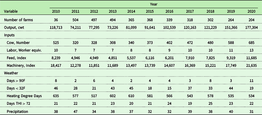
The dairy farm sector in the northeastern United States has undergone significant changes over the past few decades. One of the drivers of these changes has been a desire among many dairy producers to achieve greater efficiencies and economies of scale, because milk prices have generally not kept pace with overall US inflation (US Bureau of Economic Analysis 2020; US Department of Agriculture 2020). Although milk production has generally declined in several New England states, it has increased in New York, which remains the dominant producer in the region (USDA 2020). Even within New York, however, much of the growth in milk production has occurred on larger farms in the western portion of the state, while production has declined in more traditional dairy areas, such as the Hudson Valley. More recently, in the 2010–2018 period, both the cow inventory and milk production in New York have increased, even as the number of producing farms has declined (USDA 2020) due to a combination of attrition primarily among smaller farms and expansion of the remaining farms.
At the same time, in the Northeast, as in most areas of the world, people, plants, and livestock are facing a steady increase in average temperatures due to global warming, which could reduce agricultural output by as much as 25% (IPCC 2014). In the animal science literature, an abundance of studies shows that milk cows are sensitive to extreme temperatures. Since cows are vulnerable to heat stress, the increase in average daily temperatures and the frequency of heat waves may result in the reduction of meat and milk production (Key, Sneeringer, and Marquardt Reference Key, Sneeringer and Marquardt2014). Both daytime mean air temperatures during heat waves and low daytime temperatures have an impact on morning and evening cow milk output (West, Mullinix, and Bernard Reference West, Mullinix and Bernard2003). For New York State, the dominant dairy producer in the Northeast, the number of days exceeding 90 degrees Fahrenheit is predicted to increase five- to tenfold for the 2020s, 2050s, and 2080s (NSERDA 2014).Footnote 1 Thus, the overall expected average temperatures are increasing due to both higher frequency of very hot days and a lower frequency of extreme cold temperatures. As a result, the potential effects of extreme temperatures on dairy production efficiency via cow productivity in the Northeast remain in part dependent on the future of climate change.
This article examines the effects weather and technological change on the efficiency and productivity of farm milk production in the northeastern United States.Footnote 2 This region provides a useful case study for at least three reasons. First, farm milk production is economically important in the Northeast. In fact, it is the leading farm sector as well as the leading agricultural processing sector in terms of direct sales (Lopez, Laughton, and Jelliffe Reference Lopez, Laughton and Jelliffe2020). Thus, the efficiency of dairy farming has profound implications throughout the region’s economy and milk supply chain. Second, milk cows in the Northeast have been subject to significant variations in weather and technological change, allowing us to capture the effects of those factors on milk production and efficiency. Third, as in many other regions, home-grown feed production is an integral part of dairy cow feeding in the Northeast, and climate change is bound to affect feed production.
The contributions of this article are as follows. First, it updates estimates of the technical efficiency and productivity growth of dairy farms in the northeastern United States, which are rather dated (Tauer and Kelbase Reference Tauer and Belbase1987; Ahmad, Bravo-Ureta, and Mukherjee Reference Ahmad, Bravo-Ureta and Mukherjee1996). Second, we contribute to the growing literature on the effects of weather on the efficiency of dairy farms by considering the effects of extreme cold temperatures as well as the effects of heat on feed production.Footnote 3 To this end, we utilize an alternative measure of heat stress not used in previous dairy studies that use Temperature Humidity Index (THI) to capture heat stress. Third, we allow for input-saving technologies, rather than just Hick-neutral technical changes and, thus, for possible effects of labor-saving and other input-saving or augmenting technologies and their role in explaining changes in productivity growth in the dairy sector of the Northeast.
Using proprietary farm-level data from six northeastern states between 2010 and 2020, we apply a stochastic frontier (SF) translog production model using alternative measures of weather and find that farmers in this region are generally more technically efficient than suggested in previous studies and that extreme weather impairs technical efficiency considerably more than suggested by previous studies with older data sets or that are national in scope. We also find a benign effect of heat on feed production, which is consistent with Perez-Mendez, Roibas, and Wall (Reference Perez-Mendez, Roibas and Wall2019) for dairy production and on the effects of climate change on crops in colder areas (Jägermeyr, Müller, Ruane et al. Reference Jägermeyr, Müller and Ruane2021), such as the Northeast. Additionally, we find that dairy farms in this region exhibit significant increasing returns to scale and labor-augmenting technological changes, which support the tendency of the sector to become more consolidated and less labor-intensive.
Data
Production data
Our production data consist of proprietary farm-level milk production and financial data extracted from the annual Northeast Dairy Farm Summary (DFS) by the agricultural lender Farm Credit East, and it comprises 3,691 observations from dairy farms in the northeastern states from 2010 to 2020. Although the report is not a statistically random sample of the Northeast dairy industry, the farms are stripped of their names and randomly identified for the data analysis to preserve confidentiality.Footnote 4 Because of confidentiality concerns, the locations of the farms are only identified at the county level. The DFS has been produced for several years in a relatively consistent fashion, providing a valuable source of cross-sectional data. The data consist of balance sheet and income statement items as well as production information for each farm.Footnote 5
Output is measured by a farm’s total milk production. Inputs are divided into four categories: cows, machinery, labor, and feed. We treat cows, machinery and equipment, labor, and materials as variable inputs. Following De Loecker and Warzynski’s (Reference De Loecker and Warzynski2012) treatment of capital inputs, we treat cows as separable from other inputs and machinery as a non-separable input in the short run. Thus, our empirical model does not consider the possibility of substituting cows for machinery, labor, or feed in the short run.
For labor, the data set combines both hired labor and family labor and considers them as a single input. Small farms rely heavily on family labor, and total labor expenses are captured by the sum of hired labor expenses and family living expenses. Note that a part-time worker is considered half of a full-time worker equivalent. A feed quantity index is computed by adding up purchased feed plus crop production expenses and dividing the result by the NASS feed price index (price paid by farmers). Feed is by far the largest component of material inputs used by dairy farms in the Northeast. A trend variable (yearly trend starting from 1 in 2010 to 11 in 2020) is used to capture technical change. This trend variable is interacted with labor, feed, and machinery to capture any input-augmenting changes in technology, with a particular focus on the nature of labor-augmenting technical change.
Weather data
We collected weather information from 46 stations matching the counties where the farms in the sample are located.Footnote 6 Several measures of weather variables are considered. Following previous work, the THI is particularly useful in estimating the environmental conditions that induce heat stress (Chase Reference Chase2006). To capture potential heat stress, we measure THI at the state level. More specifically, following Chase (Reference Chase2006), THI at time t in a given location is computed as follows:
 $$\rm THI_t = dbt_t + (0.36 \times dew_t) + 41.2,$$
where dbt is the dry bulb temperature in degrees centigrade and dew is the dew point temperature in degrees centigrade at time t.Footnote 7 We utilize the number of days that the THI exceeds 72 at least once, which is the stress threshold for dairy cows (Chase Reference Chase2006). The advantage of the latter is that it captures the number of heat spells in a single variable while making it expedient to simulate optimal weather as the absence of heat spells.
Although most previous economic studies have not focused on extreme cold weather, we consider the possibility that extreme cold temperatures may affect technical efficiency and, therefore, include the average heating degree days (HDDs) at the state level (National Weather Service 2020). Extreme cold temperatures will result in high HDDs, requiring additional energy for heat, and cows will need to consume additional calories to keep themselves warm. In addition, cold weather requires increased management effort in terms of providing adequate shelter, water, health watch, and foot traction (University of Minnesota Extension 2019).
Finally, we also utilize alternative measures of extreme temperatures following the climate change measures used by NSERDA (2014) for New York State in all 46 weather stations used in the sample. For extreme heat, we use the number of days with maximum temperatures exceeding 90º Fahrenheit during a given year. For extreme cold, we use the number of days with minimum temperatures below 32º Fahrenheit.
Input prices
Regarding the prices of inputs used for the computation of allocative efficiency effects of weather changes, the price of feed used was proxied by a price index for feed published by USDA NASS (2020), the same one used to deflate purchase and crop feed expenses to compute the quantity of feed. For labor, we use the wage rate obtained by dividing labor expenses by the number of full-time worker equivalents, where family labor is valued at the opportunity cost of hiring workers. As in previous studies, we treat the number of cows as an input. The quantity of machinery is treated as a capital input, given its multi-year life span. Accordingly, we define the annual price of machinery based on the concept of the user cost of capital, that is, by adding interest for the opportunity cost of money and a depreciation rate for the annual loss of value of the capital stocks.Footnote 8 We then deflate machinery and equipment expenses by the user cost of capital.
The summary statistics of the variables in the sample are presented in Table 1.Footnote 9 The list of the 46 stations that supplied the weather data is found in Appendix A1, and the distribution of the observations across years is presented in Table A2.
Table 1. Summary statistics

Table 2. Effect of heat on feed
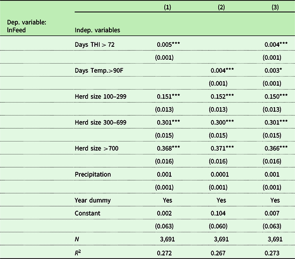
Note: Standard errors are written in parentheses. *, **, and *** denote the significance levels of 10%, 5%, and 1%, respectively.
Empirical model
Following the specification of a SF model, as in Battese and Coelli (Reference Battese and Coelli1995), to the variables assembled above, we propose the following model to estimate the effects weather on milk output:
 $${q_{it}} = {\alpha _i} + \sum\nolimits_{j} j{x_{ijt}} + \sum\nolimits_{jk} {{\beta _{jk}}} {x_{ijt}}{x_{ikt}} + \sum\nolimits_{jt} {{\gamma _{jt}}} {x_{ijt}}{T_t} + {\gamma _t}{T_t} + {v_{it}} - {u_{it}},$$
where ${q_{it}}$
is log of milk production by farm i in year t,
${q_{it}}$
is log of milk production by farm i in year t, ${x_{ijt}}$
denotes the log of the amount of input j utilized by farm i in year t,
${x_{ijt}}$
denotes the log of the amount of input j utilized by farm i in year t, ${T_t}$
denotes a time trend to capture technological changes,
${T_t}$
denotes a time trend to capture technological changes, ${v_{it}}$
is a random symmetric disturbance accounting for noise assumed to be independently, identically distributed with a mean of zero and variance
${v_{it}}$
is a random symmetric disturbance accounting for noise assumed to be independently, identically distributed with a mean of zero and variance $\;\sigma _v^2$
, and
$\;\sigma _v^2$
, and ${u_{it}}$
is an asymmetric error term that accounts for systematic deviations from the frontier due to weather shocks and unobservable factors such as management.
${u_{it}}$
is an asymmetric error term that accounts for systematic deviations from the frontier due to weather shocks and unobservable factors such as management.
Following Greene (Reference Greene2005) and Battese and Coelli (Reference Battese and Coelli1995), we use maximum likelihood to estimate equation (2) under five alternative weather measures, using the frontier command in Stata 16. We assume that the deterministic deviation from the frontier due to weather variables is separable from purely stochastic deviations. Following the best practices for SF estimation, we estimate the deterministic component to the frontier, in the same fashion as O’Donnell (Reference O’Donnell2016), by adding the variables directly into the so-called environmental variables, thus leaving the deterministic variables outside the one-sided stochastic error. This reduces the possibility of biased estimates when the stochastic term includes determinants of the deviations (Wang and Schmidt Reference Wang and Schmidt2002). Following Coelli et al. (Reference Coelli, Rao, O’Donnell and Battesse2005), we treat weather as an environmental variable that affects deviations from the production frontier. For the sake of simplicity and without loss of generality, let weather be denoted by a single variable W. Thus, ${u_{it}}$
=
${u_{it}}$
= ${\rho _\;}{W_{it}} + $ ${\varepsilon _{it,}}$
where ϵ is a one-sided stochastic component, such as management, that affects production. We then rewrite (2) as:
${\varepsilon _{it,}}$
where ϵ is a one-sided stochastic component, such as management, that affects production. We then rewrite (2) as:
 $${q_{it}} = {\alpha _i} + \mathop \sum \nolimits_j {\beta _j}{x_{ijt}} + \mathop \sum \nolimits_{jk} {\beta _{jk}}{x_{ijt}}{x_{ikt}} + \mathop \sum \nolimits_{jt} {\gamma _{jt}}{x_{ijt}}{T_t} + {\gamma _t}{T_t} - {\rho _\;}{W_{it}} + {v_{it}} - {\varepsilon _{it,}}\;$$
where the random inefficiency term ϵ follows a truncated half-normal distribution ${\varepsilon _{it}}\sim{N^ + }\left( {\mu ,\sigma _\varepsilon ^2} \right)$
.Footnote
10
This is the standard form in which THI is entered in previous studies as a measure of heat stress. However, the expression in (3) assumes that the effect of weather is independent of its effects on inputs. In our case, we need to consider the effects of weather on cows as well as feed production. To consider the first, it is reasonable to assume that weather is shared across farms in the same location, but that its effects on milk output is proportional to the number of cows. Let
${\varepsilon _{it}}\sim{N^ + }\left( {\mu ,\sigma _\varepsilon ^2} \right)$
.Footnote
10
This is the standard form in which THI is entered in previous studies as a measure of heat stress. However, the expression in (3) assumes that the effect of weather is independent of its effects on inputs. In our case, we need to consider the effects of weather on cows as well as feed production. To consider the first, it is reasonable to assume that weather is shared across farms in the same location, but that its effects on milk output is proportional to the number of cows. Let ${x_{1it}}$
denote (the log of) the number of cows in the ith farm at time t and rewrite (3) as:
${x_{1it}}$
denote (the log of) the number of cows in the ith farm at time t and rewrite (3) as:
 $${q_{it}} = {\alpha _i} + \mathop \sum \nolimits_j {\beta _j}{x_{ijt}} + \mathop \sum \nolimits_{jk} {\beta _{jk}}{x_{ijt}}{x_{ikt}} + \mathop \sum \nolimits_{jt} {\gamma _{jt}}{x_{ijt}}{T_t} + {\gamma _t}{T_t} - {\rho _\;}{W_{it}}{x_{1it}} + {v_{it}} - {\varepsilon _{it.\;}} $$
To further characterize dairy farm operations in the region, let e
i
=
 $${{\partial {q_{it}}} \over {\partial {x_{iit}}}}$$
be the output elasticity with respect to the ith input. The degree of returns to scale is given by e =
$${{\partial {q_{it}}} \over {\partial {x_{iit}}}}$$
be the output elasticity with respect to the ith input. The degree of returns to scale is given by e = $\mathop \sum \limits_i {e_i}$
, where e > 1 denotes increasing returns to scale, which in turn denotes the expected case that output expands more than proportionally to an increase in all inputs. In the short run, when intermediate capital inputs such as cows and equipment remain fixed, the short-run returns to scale can be indicated as the sum of the elasticities for labor and feed, and this is expected to be less than 1.
$\mathop \sum \limits_i {e_i}$
, where e > 1 denotes increasing returns to scale, which in turn denotes the expected case that output expands more than proportionally to an increase in all inputs. In the short run, when intermediate capital inputs such as cows and equipment remain fixed, the short-run returns to scale can be indicated as the sum of the elasticities for labor and feed, and this is expected to be less than 1.
As weather is also likely to affect feed production, the indirect effect of weather on feed must be considered. To this end, (the log of) feed is simply modeled as a function of weather and other factors and is assumed to be given by ${x_{2jt}}$
:
${x_{2jt}}$
:
 $${x_{2it}} = {\alpha _0} + {\alpha _1}{W_{it}} + \mathop \sum \nolimits_f {\alpha _{2f}}{Z_{fit}} + {\varepsilon _2},$$
where ${\varepsilon _2}\;$
are the unobservable factors with distribution
${\varepsilon _2}\;$
are the unobservable factors with distribution ${\varepsilon _2}$
∼N(0,
${\varepsilon _2}$
∼N(0, $\sigma _{{\varepsilon _2}}^2$
), and Z are other factors that affect feed production. Considering the effects through cows and feed, then, the total elasticity of milk output with respect to a percent change in a weather variable is the result of the direct effect through cow productivity and the indirect effect through feed production given by:
$\sigma _{{\varepsilon _2}}^2$
), and Z are other factors that affect feed production. Considering the effects through cows and feed, then, the total elasticity of milk output with respect to a percent change in a weather variable is the result of the direct effect through cow productivity and the indirect effect through feed production given by:
 $$d{q_{it}}d{W_{it}}{W_{it}} = \rho ({W_{it}}{x_{1it}}) + {\alpha _1}\partial {q_{it}}\partial {x_{2it}}{W_{it}} = \rho ({W_{it}}{x_{1it}}) + {\alpha _1}{e_{2it}}{W_{it}},$$
where the percent change in milk output given a 1% change in W is obtained by the sum of the direct effect through cow productivity (first term) plus the indirect effect through feed production. Note that the last term is proportional to feed elasticity of output. We estimate equation (6) for different weather variables but focus on the number of days with THI > 72 and days with temperatures >90F.
Following Coelli et al. (Reference Coelli, Rao, O’Donnell and Battesse2005), we utilize the results of model 5 in Table 3 to estimate technical efficiency scores and total factor productivity growth (TFPG). We decompose TFPG into three sources: technical changes (TCs), scale changes (SCs), and technical efficiency changes (TECs). The TC contribution is computed as the average of the partial derivatives of the output with respect to T. SC contribution is the geometric mean of two scale efficiency changes, composed of both the scale factor ( $S{F_{it}})$
and partial elasticities of production
$S{F_{it}})$
and partial elasticities of production $\left( {{e_{it}}} \right)$
multiplied by the input share, where
$\left( {{e_{it}}} \right)$
multiplied by the input share, where ${e_{it}} = \mathop \sum \nolimits_{j\ =\ 1}^J {e_{jit}}$
and
${e_{it}} = \mathop \sum \nolimits_{j\ =\ 1}^J {e_{jit}}$
and $S{F_{it}}=1 -{ \frac{1}{e_{it}}}$
. Once operational, TFPG1 = TC + SC + TEC for each farm for which we have observations for two consecutive periods.
$S{F_{it}}=1 -{ \frac{1}{e_{it}}}$
. Once operational, TFPG1 = TC + SC + TEC for each farm for which we have observations for two consecutive periods.
Table 3. Stochastic production frontier parameter estimates for northeastern dairy farms
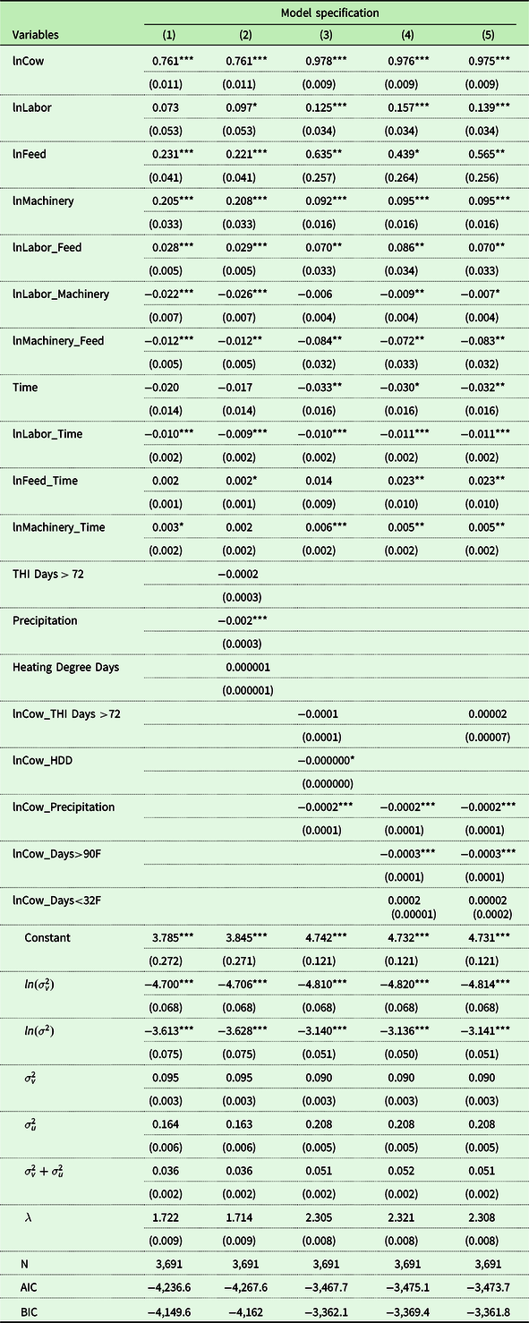
Note: Standard errors are written in parentheses. *, **, and *** denote the significance levels of 10%, 5%, and 1%, respectively.
We also estimate a measure of productivity growth that includes allocative efficiency changes (AECs). Following Kumbhakar, Wang, and Horncastle (Reference Kumbhakar, Wang and Horncastle2015), we calculate deviations of input prices from the value of their marginal products in the allocation of inputs or departures of the marginal rate of technical substitution from the ratio of input prices. Thus, deviations from cost minimization input allocations denote allocative inefficiency in an analogous way, as Farrell (Reference Farrell1957) originally defined it. Once operational, we define TFPG, considering AECs, as TFPG2 = TFPG1 + AEC.
We utilize the predicted values from the feed equation as instrumental variables for the translog equation as well as to capture impacts of climate on feed production. We utilize model 3 in Table 2 and model 5 in Table 3 for the derived measures of weather impacts, technical efficiency scores, and productivity growth. We use maximum likelihood to estimate equation (3) under alternative weather measures, using the frontier command in Stata 16. The econometric results and weather impacts, along with technical efficiency and productivity growth effects, are presented in the section below.
Results and discussion
For the computation of the elasticities of output with respect to weather on milk production, we focus on heat stress, but we also compute the elasticities for other weather variables, that is, on the number of days with THI > 72, as in previous work on climate and dairy production, and, alternatively, on the number days when temperatures exceeded 90F, as in the NSERDA (2014) study.Footnote 11
Climate effects on feed
Table 2 presents the results for three alternative models of the effect of heat stress on feed using THI-based and 90F-based measures. For control, we use farm-size categories to proxy the feed requirements based on the number of cows. We avoid using the actual number of cows because of the spurious correlation with the cow input in the translog model. We also utilize time fixed effects and precipitation. We estimated three models: (1) THI-based, (2) 90F-based, and (3) a composite model with both THI72 and 90F days. An F-test of comparison of model 3 (unrestricted) to models 1 and 2 indicates that model 3 is significantly better in explaining feed at the 0.1% level. In addition, model 1 (THI-based) is preferred to model 2 (90F-based) at the 0.1% level. In other words, THI does a better job of explaining feed than extreme temperatures when days exceed 90F. However, both measures significantly indicate that an increase in heat measure results in a larger amount of feed. This confirms a beneficial effect of heat, as found by Perez-Mendez, Roibas, and Wall (Reference Perez-Mendez, Roibas and Wall2019) for dairy production in Asturias, Spain. We also confirm the positive effect of heat on crop production in cold and northern areas reported by Jägermeyr, Müller, Ruane et al. (Reference Jägermeyr, Müller and Ruane2021). Thus, given that home-grown production is the predominant system of feed production in the Northeast, the results indicate that climate change may result in some beneficial impacts on dairy farmers.
Effects of climate change on milk output
The estimated parameters of the translog production function under various weather specifications are presented in Table 3. We estimate five alternative models: (1) no weather variables; (2) THI72 days without feed effects; (3) THI72 days with feed IV; (4) 90F days with feed IV; and (5) a composite model with THI72 and 90F days.Footnote 12 The IVs for models (3)–(5) correspond to models (1)–(3) in Table 2. Model 2 includes the number of days with THI > 72 during the year, and thus it is analogous to the way THI has been used in previous studies of climate change and dairy production in that the impact on feed is not recognized. In models (3)–(5), we interact THI72 and 90F days with the log of cows to acknowledge that the impact depends on herd size and that one size of impact does not fit all dairy operations.
Although THI is significant in the feed equation, it is not statistically significant in all versions of the milk production equations, confirming the finding of Perez-Mendez, Roibas, and Wall (Reference Perez-Mendez, Roibas and Wall2019). Model 4 includes the number of days exceeding 90F temperature, and, in fact, this variable is significant in both the feed and the translog equations. Extremely hot days have a positive effect on feed and a negative effect on cow milk productivity. Thus, at least for cold areas like the northeastern United States, the results do not support using THI to measure the negative effect of heat stress on cows. Instead, the results favor the use of the NSERDA measure of extreme heat to capture future climate change, that is, temperatures exceeding 90F.
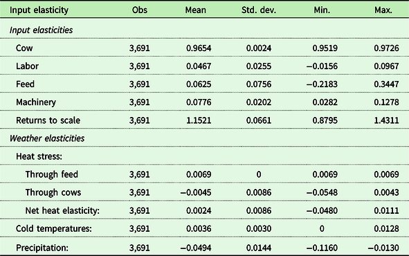
The results in Table 3 also fail to support the hypothesis that cold temperatures have a discernable impact on cow productivity. Despite studies on the negative effects of extreme cold on dairy cows, dairy cows are cold weather animals, and these effects are not picked up on an annual basis in our results. Finally, precipitation also results in lower cow productivity, which is consistent with previous studies. To gain further insight, we estimated output elasticities with respect to weather variables, as noted in equation (6). We utilize model 5 of Table 3 for this purpose. The results are presented in Table 4 and indicate that while a 1% increase in extreme heat days has a negative (−0.0045%) effect on milk output due to lower cow productivity (stemming almost entirely from 90F days), there is also a (0.0069%) increase in feed input, resulting in a rather small but statistically significant increase in milk output of 0.0024%. That is, hot temperatures from climate change can have a benign effect on dairy production systems, such as those in the Northeast, that rely on home-grown crops. The results in Table 4 also indicate that the percent increases in cold temperature have a rather small effect on milk output. On the other hand, precipitation has a negative effect on milk output as measured by an elasticity of −.0494, basically equivalent to the mean elasticity for heat stress on direct cow production.
Table 4. Estimated input and weather elasticities of output
The above results contrast with the very modest effects of extreme heat (THI) on cow productivity estimated by Key, Sneeringer, and Marquardt (Reference Key, Sneeringer and Marquardt2014), who, using a THI-based measure and a national sample, concluded that heat stress effects on technical efficiency are under 1% for the three northeastern states that constitute their Northeast region. In addition, we conclude that cold weather temperatures do not have a discernable effect but also suggest consideration of the potential effects on feed production and alternative measures to THI > 72 to measure heat stress.
Technology results
From the results in Table 3, we compute the output elasticities with respect to inputs and present the results in Table 4. Their sum indicates that farmers in the Northeast experience significant returns to scale, estimated at 1.16 at mean values, which is statistically significant at the 0.01% level. That is, if all inputs are doubled, milk output more than doubles. This characterization of technology supports the ongoing consolidation in the region’s dairy farm sector.
Another result of interest is that technical change (time) interacted with labor has a negative sign and is practically unchanged across model specifications, indicating labor-saving technical change. Technology is evolving in ways that save farm labor, although machinery and equipment did not produce any measurable interaction with technology in the time span of our sample. It is also interesting to note the increasing importance of feed as a dominant non-cow input in dairy production, as indicated by the interactions of the log of feed and time, which are statistically significant at the 5% level.
Based on the results for model 5 in Table 3, we computed technical efficiency scores. The average score of technical efficiency across all farms is estimated at approximately 0.86 out of a maximum of 1.0 for firms to be on the frontier, with a minimum of 0.49 and a maximum of approximately 0.98. In other words, the average northeastern dairy farmer obtained 86% of potential output using their capital, labor, and materials, a loss of about 14% from the ideal output obtained for the same set of inputs.Footnote 13 As compared to previous studies on technical efficiency, dairy farms in the Northeast reach a higher level than in the past, 69% for New York dairy farms (Tauer and Belbase Reference Tauer and Belbase1987), 85% for Pennsylvania dairy farms (Wang Reference Wang2008), and 82% for New England dairy farms (Ahmad, Bravo-Ureta, and Mukherjee Reference Ahmad, Bravo-Ureta and Mukherjee1996).
Productivity growth results
The results for the decomposition of productivity growth changes between 2010 and 2020 are presented in Table 5. Note that these measures were computed at the farm level and thus include observations only for those farm records that were observed in consecutive years. Table 5 indicates that much of the productivity growth came from changes in technology, with average small negative effects of changes in scale and technical change over the whole sample. Technical change increased productivity by an average just over 1% per year (1.04% in the farm-weighted average), making technical change the largest contributor to productivity growth. Changes in technical efficiency and allocative efficiency contributed negatively to productivity growth. Overall, based on the 2011–2020 average using the number of farms as weights, TFPG increase at a rate of approximately 1% (TFPG1 = 0.98) and when allocative efficiency effects are included to obtain TFPG2, the average productivity drops to 0.65.
Table 5. Mean total factor productivity growth by year
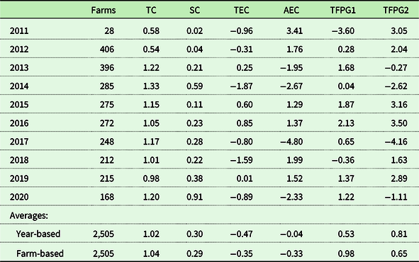
Notes: The TC = technical change; SC = scale efficiency change; TEC= technical efficiency change; AEC= allocative efficiency change; TFPG1 = TC + SC + TEC and TFPG2 = TFPG1 + AEC. The farm-based averages are the weighed averaged based on the number of farms in the full sample while the year-averages are the simple averages across the means for each year.
As shown in Table 6, when the productivity growth results are broken down by size categories based on the number of farms, it is interesting to note that smaller farms (<100 cows) are the only ones to exhibit negative effects of scale efficiency, although they exhibit the second highest technical change effects among the four size groups. In contrast, larger farms (>700 cows) exhibit the highest scale effects but the lowest effects from technological change. Overall, considering technology, scale, and technical efficiency changes, results show that the largest farms (>700 cows) exhibit the highest productivity growth rates per year (TFPG1 = 1.62). Farms with less than 300 cows exhibit either the lowest TFPG (<100 cows with TFPG1 = 0.01) or the lowest TFPG when allocative efficiency effects are considering (100–299 cows with TFPG2 = 0.27). This group also exhibits the highest productivity growth rates when AECs are taking into account. This suggest that that small- to medium-size operations are more likely to struggle to catch up in productivity with larger operations and also to allocate inputs in a manner consistent with cost minimization. This provides an opening for policy and managerial support to support small- to mid-size dairy farms to enhance their productivity growth to overcome scale disadvantages as well as better achieve allocative efficiency.
Table 6. Total factor productivity growth by herd size
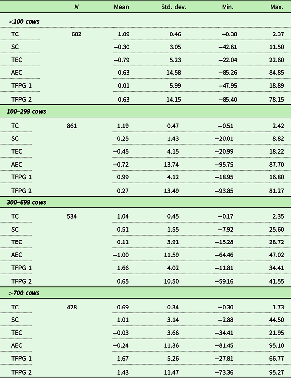
Notes: TC = technical change; SC = scale efficiency change; TEC= technical efficiency change; AEC= allocative efficiency change; TFPG1 = TC + SC + TEC; TFPG2 = TFPG1 + AEC.
Conclusion
Adverse weather effects, which may be exacerbated by climate change, can significantly affect the productivity of dairy farms in the Northeast. Previous work focusing on weather effects in the northeastern dairy farm sector has focused on heat stress in cows, side-stepping effects on feed production, and is either dated and/or has utilized aggregate data. In this article, we ascertain the effect of heat stress as well as cold temperatures on milk productivity, accounting for effects on feed production and labor-augmenting technology. The empirical framework involves the use of a SF production function applied to farm-level data between 2010 and 2020.
In general, the empirical findings are consistent with previous studies reporting that heat stress reduces efficiency and in terms of the production function estimates. However, we do not find support for using THI as a measure to capture heat stress effects on cows in cold areas such as the Northeast but do find that it captures effects on home-grown feed production. We find heat stress, as measured by the number of days exceeding 90F, to have a detrimental effect on cow productivity but that heat stress, measured either by THI > 72 or 90F days, has a beneficial effect on feed production and an overall net positive effect on milk production. We also fail to find a discernable effect of cold temperatures on milk production. From a technological standpoint, we also find evidence of significant returns to scale, labor-augmenting technical change, and a rather modest level of productivity growth of approximately 1%, on average. In general, we find technical efficiency scores that are higher than those estimated in previous studies.
From a productivity standpoint, this paper offers some useful insights. The results confirm the presence of significant increasing returns to scale. Productivity growth rates across herd sizes reveal that scale efficiency is the greatest advantage of larger operations and the most disadvantage of smaller ones, even though smaller operations experience comparable or effects of technical changes on productivity rates than other groups. On average, the sector experience approximately a 1% TFPG per year mostly due to technical change, secondly due to scale efficiency, and with negative contributions of technical and AECs over the period. Another interesting finding is that the sector is experiencing labor-augmenting technical change, which is leading to a less labor-intensive production technology.
This paper has limitations due, in part, to data availability. Although we used a farm-level confidential data set, we did not have access to individual farm characteristics (e.g., precise location) or characteristics of the operators (e.g., age, experience, etc.) that may explain large variations in technical efficiency and productivity measures that remained unobserved. For instance, efficiency effects varied quite substantially (0.53 to 0.98) in the sample. Although one can rightly attribute this to variations in management, we do not have any individual farm data to measure this effect. Another data-related issue is the measurement of weather converted to annual data to match the paucity of the farm records at the county level. Obviously, weather varies substantially within a year, and a more granular measure of farm records and weather would fine-tune the weather effects. A longer time series would obviously provide a better assessment of long-term effects of temperature and climate change, as these changes are gradual. However, these limitations provide opportunities to expand the methods of this paper to other regions or farm sectors where climate change and weather also have the potential to significantly affect the productivity of future farm operations.
Data availability statement
The farm-level data utilized under a confidentiality agreement between Farm Credit East and the researchers, and it is not available to third parties. Note that Farm Credit East collects these data from farmers under a pledge of confidentiality. However, the computer codes and the weather data are available from the authors upon request.
Funding statement
This work was supported by USDA National Institute of Food and Agriculture, Hatch project accession number 1020636, and the Richard DelFavero Fund for Agricultural and Resource Economics at the University of Connecticut.
Competing interests
The authors have no conflict of interests regarding the research reported here.
Data Appendix
Table A1. List of weather stations used in the sample

Table A2. Mean values of observations over years


 Open access