


1. Introduction
Because both snow and ice have a high albedo and effectively insulate the ocean from the atmosphere, it has generally been accepted that changes in ice-pack extent and thickness will have an amplified effect on climate through the albedo feedback mechanism (Reference Ingram, Wilson and MitchellIngram and others, 1989; Reference LedleyLedley, 1991; Reference Manabe, Stouffer, Spelman and BryanManabe and others, 1991; Reference Rind, Healy, Parkinson and MartinsonRind and others, 1995). The extent and thickness of the snow and ice cover of the Arctic basin are controlled in large measure by the regional heat budget. Changes in the budget will lead to changes in ice extent, with a warming climate potentially producing a much diminished ice cover. As a consequence, the Arctic Ocean heat budget has both regional and global significance. It is not surprising, therefore, that the heat budget has been studied for more than 40 years (Reference UntersteinerUntersteiner, 1961; Reference Doronin and KheisinDoronin and Khesin, 1977). Most recently, a year-long project, Surface Heat Budget of the Arctic Ocean (SHEBA; Reference PerovichPerovich and others, 1999a, Reference Perovichb), was undertaken to better understand the processes governing the exchange of energy between the ocean and the atmosphere.
As part of SHEBA, time-dependent measurements of snow depth (h), ice thickness (h) and the temperature of the snow-ice interface (21) were made at 30 locations in a variety of ice and snow conditions using mini dataloggers. It has been shown (Reference Maykut and UntersteinerMaykut and Untersteiner, 1971; Reference MaykutMaykut, 1978) that between November and April, heat conduction through the ice and snow (Fc) is a major component of the surface energy budget, balancing winter losses to the atmosphere via longwave radiation and turbulent fluxes. Using data from the 30 sites, we have calculated fc. While snow depth and ice thickness are known controls on fc, their impact on the heat flow from the ice has mainly been investigated using models and theory. Here, we present empirical results and compare them to our theoretical understanding. The results show that in the natural system there is a high degree of spatial variability, with four-fold variations in fc occurring over distances of tens of meters. This variability is so large as to suggest that it may need to be considered when estimating heat fluxes over large aggregate areas.
2. Location, Instruments and Methods
The SHEBA camp was established on the ice of the Beaufort Sea at 75° N, 142° W in early October 1997 and then drifted until October 1998, at which time it had reached 80° N, 162° W. Standard ice-thickness and snow-depth stakes (Reference UntersteinerUntersteiner, 1961; Reference HansonHanson, 1980; Reference Perovich and ElderPerovich and Elder, 2001) were established around the camp and measured weekly throughout the winter (Reference PerovichPerovich and others, 1999a, Reference Perovichb). At 30 locations, grouped into three basic clusters, mini dataloggers (Hobo-XT, Onset Computer Corp.) were installed on selected stakes, with an external thermistor placed at the snow-ice interface about 25 cm from the stake base. The thermistors were covered in white heat shrink, but otherwise unshielded. The mini dataloggers recorded the temperature of the interface every 2.4 h throughout the winter with an accuracy of 1.0°C (cf http://www.onsetcomp.com; http://arcss.colorado.edu/Catalog/arcss001.html). Data were collected by the loggers between October 1997 and May 1998. Two of the 30 loggers were lost during a period of intense ice deformation. Another two failed part way through the winter and could not be used in our analysis, leaving 26 record sets.
The dataloggers were installed in three basic clusters: (1) at "Baltimore" (Fig. 1a): an abrupt transition from hummocky and slightly ridged ice to thinner first-year ice; (2) at "Seattle" (Fig. 1b): an area of melt ponds separated by white ice hummocks; and (3) at "the Ridge" (Fig. 1c): a 1.5 m high ridge in a multi-year floe. The sites were named after cities for convenience. At Baltimore, six dataloggers were installed, three in hummocky, deformed ice, three in the adjacent young ice. Of these latter three, two ended up located under a thick drift that formed in the lee of an 80 cm high section of deformed ice. At Seattle, five dataloggers were installed. One of these was placed on top of an ice hummock. The others were located so that they recorded snow-ice interface temperatures from refrozen melt ponds which usually fill with snow early in the winter (Reference Perovich and ElderPerovich and Elder, 2001; Sturm and others, in press b). At the Ridge, 19 dataloggers were installed along a transect that ran transverse to the ridge axis. This transect was about 100 m long and extended from undeformed ice south of the ridge to undeformed ice north of it. A more detailed description of the sites, as well as ice-thickness, snow-depth and interface temperature data are available on CD-ROM (Reference PerovichPerovich and others, 1999a).

Fig. 1. (a) cross section showing the snow and ice surfaces at the baltimore cluster. locations of stakes and min dataloggers are shown. stake numbers are denoted by "g", and datalogger numbers by "h", the top panel shows spot measurements of snow-ice interface temperature taken 14 april 1998 when the air temperature was −13°c (b) cross-section showing the snow surface and the ice surface and base at the seattle cluster. locations of stakes and mini dataloggers are shown, (c) cross-section showing the snow surface and the ice surface and base at the ridge cluster. the top panel shows spot measurements of the snow-ice interface temperature taken 1 april 1998 when the air temperature was −15°c
We focus on the winter period 15 November-30 April, which corresponds with the part of the year when conductive heat fluxes dominate the heat budget. Dataloggers were installed in late October at Seattle and the Ridge, but we were unable to install the dataloggers at Baltimore until 11 December. For this site, 26 days at the beginning of the winter period are missing. We correct for this omission where necessary as follows: for all sites other than those at Baltimore, we compute average values for the period 11 December-30 April, as well as for the full winter period. Comparing the two averages, we compute a correction for the early winter period. For example, the extra 26 days in early winter increased the interface temperature by about 0.5°C in most cases. The corrections are applied to the Baltimore records, but in most cases are insignificant.
In April 1998, extensive measurements of snow depth, density, stratigraphy and thermal conductivity were made near the dataloggers as well as in many other locations around the SHEBA camp (Sturm and others, in press a, b). Snow measurements were made at six locations at Seattle, twelve locations along the Ridge transect, and six at Baltimore. The average bulk thermal conductivity (ks) for vertical heat flow was determined for each cluster using layer stratigraphy, layer density and the results of 89 needle-probe measurements of thermal conductivity (Reference Sturm, Morris, Massom and JeffriesSturm and others, 1998, in press a) keyed to individual strata. Snowpack properties for each site are listed in Table 1. As might be expected from the site descriptions, the snow at Baltimore was the deepest and densest due to drifting. It was least deep and dense at Seattle where melt-pond in-filling produced less wind slab than at the other sites. These depth and density differences may account for the slightly lower value of ks at Seattle. In general, however, snow conditions and thermal conductivity values were similar at the three clusters.
Table 1. Snowpack properties at the three clusters where mini dataloggers were located

Air temperature was measured continuously at the Seattle site using a Campbell GR-10. The Ridge site was about 0.4 km and the Baltimore site > 4 km from the Seattle site. The Seattle air-temperature record, however, was found to be within 1 ° or 2°C of air temperatures collected at several other sites within a 5 km radius (Reference Claffey, Andreas, Perovich, Fairall, Guest and PerssonClaffey and others, 1999; Reference Perovich and ElderPerovich and Elder, 2001), so we use it as the "standard" air temperature at all sites.
For calculation of temperature gradients across the snow, we assume that snow surface and air temperatures were the same. Both direct and indirect data suggest this is reasonable. In his careful and pioneering study, Reference NybergNyberg (1938) found that on cloudy days, or clear days when the wind speed was > 1.75 m s−1, <0.4°C difference existed between air and snow surface temperatures. Reference Guest, Davidson, Johannessen, Muench and OverlandGuest and Davidson (1994), working on Arctic sea ice, also found that surface inversions were relatively infrequent and, even when present, produced differences in air and surface temperatures that did not exceed 2°C. They concluded that under windy, cloudy conditions, much smaller differences (≪1°C) were likely. Given that the mean wind speed at SHEBA for the period used in our calculations was 4.7 ms−1, and >89% of all hourly wind-speed measurements exceeded 1.75 ms−1, we think that any differences that existed were small. Contributing to this reduction, we note that it was virtually always cloudy at SHEBA.
We have estimated the difference between air and snow surface temperature directly using hourly measurements from a vertical thermistor string. The upper part of this string was exposed to the air while its lower part was embedded in the snow. The mean difference between the temperature recorded at a height of 50 cm, which was generally within a few centimeters of the snow surface, and the temperature at 100 cm height (effectively the air temperature) was 0.45°C (n = 3996). Maximum differences were about 2°C, but these occurred < 2% of the time. Since the difference between the temperature at the snow surface and the snow base (snow-ice interface) generally ranged from 10° or 15°C, our assumption that the snow surface and air temperature were the same results in errors in vertical temperature gradient of only about 5%. We think this small error is acceptable given the rough nature of our heat-flux estimates.
3. Results
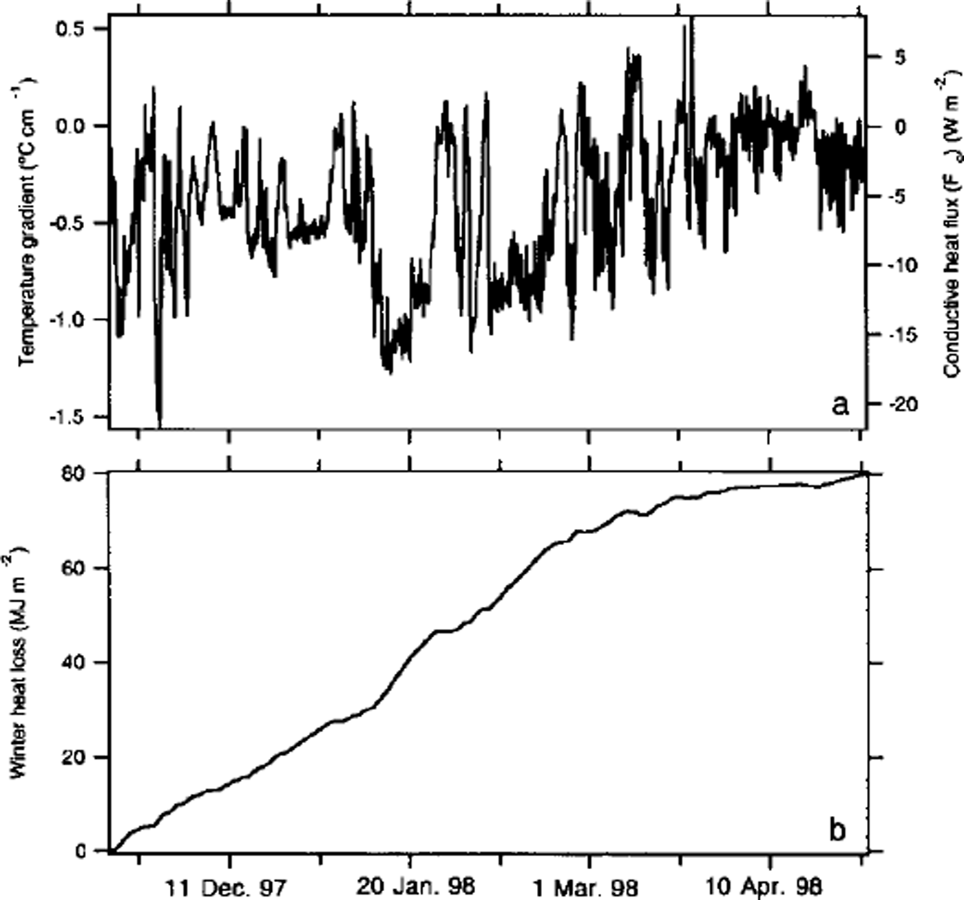
A typical set of records, in this case from stake 9 (datalogger 19) on the Ridge (see Fig. 1c), are shown in Figure 2. They indicate that the interface was considerably warmer than the snow surface throughout the winter, sometimes by as much as 15°C. The difference between the air and interface temperature, divided by the snow depth, gives the vertical temperature gradient. It is proportional to the vertical conductive heat flux, with large negative gradients leading to upward heat flow across the snowpack. At stake 9, where the snow depth increased from about 12 cm to 30 cm between 15 November and 30 April (the start and end of winter), the increase in depth was not monotonic, and as a result the temperature gradient evolved in a more complex manner than would normally be the case from air-temperature fluctuations alone. A wind slab deposited in early December increased the snow depth by 16 cm, but was subsequently eroded away in January. Similar erosion of the snowpack was observed at about half of the datalogger sites (marked by "e" in Table 2). The record in Figure 2 also indicates that the ice at stake 9 increased in thickness about 100 cm over the winter, slightly unusual for a spot where the ice was already > 200 cm thick in the autumn. At some of the other sites, particularly those near the crest of the Ridge where the ice was > 400 cm at the start of winter, the thickness actually decreased over the winter.

Fig. 2. Bottom: snow-ice interface and air-temperature records from stake 9 ( datalogger 19). see table 2 for statistics and figure le for location. middle: snow-depth record from stake 9. top: ice-thickness record from stake 9.
Table 2. Summary statistics for datalogger sites
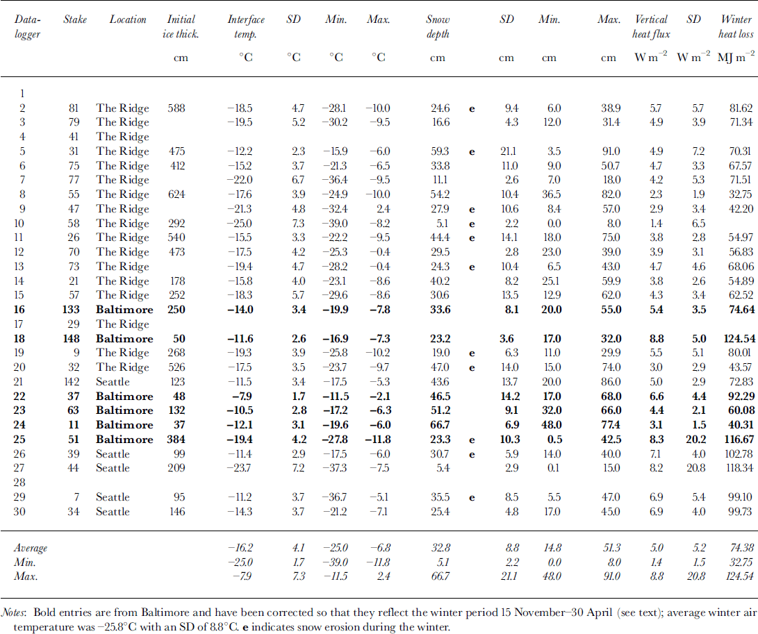
In Table 2 we have compiled temperature, snow-depth and heat-flux statistics for all sites, and in Figure 3 we have plotted the lowest, highest and average interface temperature records for winter 1997/98. The average interface temperature at stake 9 (the example in Fig. 2) was −19.3°C, slightly lower than the average for all the sites. For comparison, the average air temperature for the same period was −25.8°C. Perhaps the most noticeable result is that the range of average interface temperatures was large, extending from −7.9° to −25°C. This range indicates a high degree of spatial variability, and as we will show shortly, implies a high degree of spatial variability in vertical conductive heat fluxes from the ice. Spot measurements (i.e. top panels in Fig. 1a and c) made at the datalogger sites as well as at a dozen other locations at SHEBA confirm that wide variations in snow-ice interface temperatures were common, with the range of temperatures often exceeding 20°C over distances of < 100 m

Fig. 3. The lowest, highest and average interface temperature records from sheba, winter 1997/98.
The standard deviations (SD) of the interface temperature (Table 2), a good measure of how much the snowpack damped the fluctuations in air temperature, also can be seen to have varied widely from site to site. In general, SD varied inversely with the average interface temperature. Sites with low interface temperatures had high SD values because there was little snow to attenuate or damp the wide swings in air temperature, while sites with high average interface temperatures had low SD values.
The time-averaged snow depths (Table 2) also showed marked variability and a direct relationship to average interface temperatures; sites with greater than average depths had higher than average temperatures (Fig. 4). This positive relationship between depth and interface temperature is also nicely illustrated in Figure lc, where the drifted snow on the north (lefthand) side of the Ridge is deeper than the snow on the south side, and the interface temperatures (Fig. 1c, top panel) are correspondingly higher. A similar relationship can be seen at Baltimore (Fig. 1a, top panel). These examples, however, obscure some of the complexity in the relationship between snow depth and interface temperature. It is actually the time-varying depth, not the average depth, that controls the interface temperature, and as Figure 2 illustrates, the time-varying snow-depth history can be quite complex. We think this may be part of the reason why the scatter, particularly at greater depths, is so high in Figure 4. We note that the mean end-of-winter snow depth at SHEBA was 33 cm (Sturm and others, in press b). This suggests that depths of > 33 cm were likely to be the result of wind transport and drifting of snow. Drifting is a complex and spatially heterogeneous process, and one that occurs frequently in a windy place like the Arctic Ocean. This complexity and heterogeneity is suggested in Table 2 where more than half the datalogger sites experienced a significant erosion of snow (>15 cm removed) ( "e" in Table 2) sometime during the winter.

Fig. 4. Average winter interface temperatures as a function of average winter snow depths. numbers indicate datalogger and correspond with numbers in table 2 and "h" numbers in figure la-c. the mean winter air temperature for the same period is shown at zero depth by the black circle.
4. Analysis
Temperature and snow-depth records, like those shown in Figure 2, can be used to estimate the vertical conductive winter heat flux (Fc) at each datalogger site. To do so, we assume that at each site we have a layer of snow of thickness h overlying a slab of ice, that the heat flux out of the ice and into the snow is strictly vertical and that the temperature profile in the snow is linear. Under these conditions we can write:

where ks is the thermal conductivity of the snow, Ti is the temperature of the snow-ice interface, and t0 is the surface temperature of the snow, here approximated by the air temperature. We can estimate the total conductive heat loss over the winter for each site by integrating Equation (1):

For these calculations, we use a fixed value of ks equal to 0.14 W m−1 K−1, which is close to the values determined by direct measurements at each cluster (Table 1). We think that the use of a fixed value is justified because the range of all values observed at SHEBA was small; at 194 locations, the mean value of ks at SHEBA was 0.14 with a standard deviation of only 0.03 W m−1 K−1. In another paper (Sturm and others, in press a) we discuss why this value differs from the more commonly used value of 0.3 W m−1 K−1. Briefly, the higher value was introduced 30 years ago by Reference Maykut and UntersteinerMaykut and Untersteiner (1971). It was based on measurements made by Reference Abel’sAbel’s (1893) on terrestrial snow. Fortuitously, this higher value produces reasonable equilibrium ice thicknesses when used in a thermodynamic model. As a result, its use has been perpetuated in subsequent models. However, the higher value is actually an effective value and probably appropriate only when applied over larger areas of sea ice than at a single point. At this larger scale it is not clear how the appropriate vertical temperature gradient should be determined, but it is likely to be some sort of spatially averaged gradient. Here, where the main focus is local values of heat flow and inter-site comparison, we prefer to use directly measured values of ks and note that even if we did use the higher value of ks, it would change the magnitude of our results but not the relative differences between sites.
Representative computations for stake 9 at the Ridge (see Fig. 1c for its location and Fig. 2 for the forcing data that were used) are shown in Figure 5. The computed temperature gradient ((Ti - t0)/h) (Fig. 5a, left axis) has been converted to fc (Fig. 5a, right axis) by multiplying by ks. The integrated heat loss as a function of time, JT (Equation (2)), is shown in Figure 5b. The effect of erosion of snow from the site in January (Fig. 2) is clearly evident as an increase in the rate of heat loss in January, and this accelerated rate continues until March. At that time further accumulation of snow and a decrease in the temperature gradient due to higher air temperatures reduced fc, and the rate of heat loss slowed down, but not before the erosion had significantly increased the total loss for the winter. Results from similar calculations for all the sites are listed in Table 2. Once again, corrections have been applied to the data from the Baltimore sites using an approach similar to that used for the average interface temperature. For average heat flux (Fc), the values for Baltimore have been increased by 0.30 W m–2, again an insignificant change, but one that is consistent with the fact that interface temperatures were 0.5°C higher in early winter. For estimates of JT, we have computed how much of the total heat for the winter was lost between 15 November and 11 December at sites other than Baltimore: the amount was 20 ± 5% of the total. Values for Baltimore have been increased a corresponding amount.
Based on the results of the heat-flux computations (Fig. 6), we find that winter heat losses varied by a factor of 4 across all three datalogger clusters, with the losses at each local cluster being nearly as large as the losses across all of the clusters combined. At the Ridge site, for example, heat losses varied by a factor of 2.5, and the two extremes were < 20 m apart. At Seattle, the factor was 1.6, but the extreme values were found < 10 m apart. At Baltimore, the factor was 3.1, again over a distance as short as 20 m. Moreover, in this last case, the maximum and minimum were both located in an area of young ice, so the large range was not the result of a transition from one ice type to another. This spatial variability is unlikely to be the result of systematic variations in the thermal conductivity (ks) of the snow. As indicated in Table 1, measured differences in ks between sites were small. More likely, variations in snow depth were the main cause of the wide range in heat-flow values. These results emphasize the spatial heterogeneity of vertical conductive fluxes, not only between floes, but also within small areas on a single floe.

Fig. 6. Total accumulated winter heat loss ( jt) as a function of average winter snow depth. the different symbols correspond to the three clusters where dataloggers were located. the solid line is a linear fit to all the data. the dashed and dot-dashed lines are fits to the ridge and seattle data, respectively. the light dotted line shows that the relation between JT and depth for the baltimore sites differs from the other two sites, e indicates sites at which significant snow erosion occurred during the winter. the pattern from the baltimore site is confusing, in large measure because at baltimore two very different types of ice were adjacent to each other.
There was a tendency for the heat-loss data to group by ice type. A linear regression fit to all heat-loss data as a function of snow depth (Fig. 6, solid line) had an r2 of 0.30 and there was considerable scatter, but improved regressions and less scatter resulted when data from single clusters were used. For example, at the Seattle and Ridge sites, each of which was comprised of mainly one type of ice (multi-year deformed ice at the Ridge; hummocky and ponded ice at Seattle), r2 values of 0.78 and 0.61, respectively, result when the data are used separately. Interestingly, the slopes of these lines are the same as the slope of the line fit to all of the data, though their intercepts are different. The intercept is higher for the Seattle site than the Ridge site, implying that if there had been no snow cover at either site, the total heat loss from Seattle would have been 4 3% greater than at the Ridge. This is consistent with the fact that the ice was 3 times thicker at the Ridge than at Seattle (average ice thickness at start of winter: 431 cm vs 124 cm, respectively). Surprisingly, despite the fact that at individual sites the erosion of snow during winter led to a definite increase in heat loss (Figs 2 and 5), no systematic pattern of heat loss vs erosion is apparent (Fig. 6, sites marked with "e" ) .
5. Discussion
It is well known that the conductive heat flux from the ocean to the atmosphere, fc, is controlled by snow depth (h), snow thermal conductivity (ks), ice thickness (h) and ice thermal conductivity (ki). This dependence has been investigated theoretically and solved analytically, but almost always for the case of one-dimensional, vertical heat flow. Reference MaykutMaykut (1978) provides an extensive discussion of the interrelationship between these four critical parameters and derives a formula for the heat flux using them:
where 7 is equal to kiks/(ksh + kih), and Tb is the temperature at the base of the ice. Maykut’s solution (Equation (3) here) provides a convenient way to compare our empirical results to our understanding of the conductive heat flux based on theoretical considerations. These two computed fluxes differ fundamentally in that the empirical results include the influences of spatial heterogeneity, lateral heat flow and possibly even non-conductive heat-transfer processes, while the theoretical results are one-dimensional and strictly conductive. We have solved Equation (3) using a value of ki equal to 2.0 m−1K−1, ks equal to 0.14 W m−1 K−1, T0 equal to −25.8°C, Tb equal to −2°C, and the range of average snow-depth and ice-thickness values actually present at SHEBA (5 cm < h < 67 cm; 35 cm < h < 625 cm). The results define a curved field (Fig. 7a) with increasing values of fc at decreasing values of snow depth and ice thickness. This field defines the theoretical impact of ice thickness and snow depth on the heat flow.

Fig. 7. Wmter conductive heat flux (fc) computedfor the range of winter snow depths and ice thicknesses observed at sheba, based on (a) a one-dimensional theoretical heat-flow equation (equation (15) in Reference MaykutMaykut (1978) and equation (3) here), and ( b) based on the empirical results listed in table 2.
In contrast, the observed results define a much less regular surface (Fig. 7b) that suggests a more complicated dependence of fc on snow depth and ice thickness. The overall magnitudes of the two sets are comparable, but differ in detail. For the case of thin snow and thin ice, values predicted using Equation (3) are several times higher than any values observed, in part because our sample set did not include much thin ice. For the case of thick snow and ice, observed values of fc are somewhat higher than predicted. The rapid exponential rise in fc for very thin snow and ice predicted by theory does not appear, nor is it suggested, in the observed data. Instead, there appears to be flattening at thinner snow and ice values. Similarly, over most of the range of ice thickness, but particularly for thinner ice, the observed increase in fc with decreasing snow depth is more rapid than predicted, especially in the snow-depth range 60−20 cm. We note that with a mean depth of 33 cm, nearly all of the surface area of ice at SHEBA falls within this depth range. Essentially, our observed data define a less extreme conductive heat-transfer system than suggested by the theoretical results, with higher values of fc where the snow is thicker, and lower values of fc where the snow is thinner. The observed data also show a more distinct dependence on ice thickness.
We speculate that the differences between observed and predicted heat flow arise because of the complex three-dimensional geometry of the snow and ice. We think this geometry results in significant horizontal transport and focusing of heat, a process not accounted for at all in one-dimensional Equation (3). Because of the 10:1 ratio between ks and ki wherever ice hummocks or ridges displace snow and result in thinner snow cover, fc heat-flow vectors converge (Sturm and others, in press a). Rather than being negligible, this horizontal transport of heat results in significant variations in heat flow on the scale of the ice and snow geometry, a scale that is on the order of tens of meters or less, leading to variations in vertical heat flow over small spatial scales. We suggest that this spatial variability may need to be considered when scaling up heat fluxes from point measurements to aggregate scales.
6. Conclusions
Continuous winter measurements of the temperature of the snow-ice interface from the Beaufort Sea during project SHEBA showed a wide range of variability. Temperatures on average were 10°C higher than the air temperature, but at individual locations, often only tens of meters apart, the average temperature could be 1 °C or as much as 17°C higher than the air temperature. A linear relationship was found between the winter average interface temperature and winter average snow depth, but the scatter at greater depths was high, probably because sites with deeper snow had a complex history of snow accumulation and erosion that led to large variations in heat flux through the winter. Using continuous records of interface and air temperature from 26 sites, the winter conductive heat flux, fc, was calculated, and the total heat loss for the winter for each site was computed by integrating fc. Heat losses varied by a factor of 4, and sites just a few tens of meters apart showed differences as great as those hundreds of meters apart. These results highlight the importance of small-scale spatial variability of the snow and ice for the winter heat flux. Comparison of our results with theoretical calculations suggests that due to small-scale variations in heat flux arising from horizontal transport of heat, the flux is a more complex function of snow depth and ice thickness than would be predicted by theory.
Acknowledgements
This work was funded as part of the SHEBA program by the U.S. Office of Naval Research High Latitude Physics Program and the U. S. National Science Foundation Arctic System Science Program. We thank the crew of the Canadian Coast Guard ice-breaker des groseilliers, along with the logistics group from the University of Washington Applied Physics Laboratory for their superb support during the SHEBA field program. B Elder, J. Richter-Menge, W. B. Tucker, III, T. Udall, H. Eiken, T Grenfell and B. Light assisted in collecting snow and ice measurements. P. Langhorne provided fine editorial advice.


