


1. Introduction
Improved understanding of the mixing mechanisms of fluids in a porous medium is of relevance to a wide range of applications in hydrology, water resources engineering, enhanced oil recovery, geothermal systems and risk analysis of groundwater pollution. Several factors impact the spatiotemporal transport dynamics of a solute injected in a fluid-saturated porous medium. These factors consist of properties characterising both the injected fluid and the porous medium, including properties of the ambient fluid flowing through the medium. Another important factor is the initial configuration of the injected solute, in particular, its geometrical shape. These factors can introduce disorder in the flow field as they modulate the strength of physical processes such as advection and diffusion. In this work, we investigate how the initial configuration of the injected fluid and the mean flow velocity, e.g. the mean groundwater velocity, control the relative impact of multiple sources of disorder on the mixing evolution of two miscible fluids, i.e. the ambient fluid and an injected solute. The main sources of disorder examined in this study are the viscosity and density contrasts between the injected solute and the ambient fluid. We also analyse the effect of a third source of disorder, permeability heterogeneity of the porous medium, in the form of stratification or layering.
Much of the previous work focused on the effects of permeability variability on mixing (e.g. Le Borgne, Dentz & Villermaux Reference Le Borgne, Dentz and Villermaux2015; Dentz et al. Reference Dentz, de Barros, Le Borgne and Lester2018) and dispersion (e.g. Dagan Reference Dagan1984; de Barros & Rubin Reference de Barros and Rubin2011). This is due to the fact that the variability of the permeability field over multiple length scales leads to enhanced solute mixing (Dentz et al. Reference Dentz, Le Borgne, Englert and Bijeljic2011; Bonazzi, Dentz & de Barros Reference Bonazzi, Dentz and de Barros2022). However, other mechanisms can impact solute mixing and spreading rates. For example, differences in viscosity between the added solute and the ambient fluid impact the mixing dynamics in porous media. When the injected fluid is less viscous than the ambient fluid, fluid displacement can lead to the formation of a hydrodynamic interface instability denoted as the Saffman–Taylor instability. This hydrodynamic instability generates viscous fingering (Saffman Reference Saffman1986; Homsy Reference Homsy1987) which can potentially augment dilution rates (Jha, Cueto-Felgueroso & Juanes Reference Jha, Cueto-Felgueroso and Juanes2011b, Reference Jha, Cueto-Felgueroso and Juanes2013). For many miscible flow systems, the viscosity of the fluid mixture depends on the the volume fractions of the individual fluids. In the case of injected solute–ambient fluid systems, this is equivalent to the mixture viscosity's dependence on the injected solute concentration. As a result, the solute plume's mobility and, consequently, mixing are significantly affected by the viscosity contrast (Jha, Cueto-Felgueroso & Juanes Reference Jha, Cueto-Felgueroso and Juanes2011a; Nijjer, Hewitt & Neufeld Reference Nijjer, Hewitt and Neufeld2018; Tran & Jha Reference Tran and Jha2020, Reference Tran and Jha2021; Bonazzi et al. Reference Bonazzi, Morvillo, Im, Jha and de Barros2021). The interaction between viscosity contrast and permeability heterogeneity and its effect on mixing have been studied for low levels of heterogeneity (Tan & Homsy Reference Tan and Homsy1992; Tchelepi & Orr Reference Tchelepi and Orr1994; De Wit & Homsy Reference De Wit and Homsy1997a,Reference De Wit and Homsyb; Nicolaides et al. Reference Nicolaides, Jha, Cueto-Felgueroso and Juanes2015; Bonazzi et al. Reference Bonazzi, Morvillo, Im, Jha and de Barros2021). These studies shed light on how and when solute mixing is affected by the fluctuations of the permeability field. Through the use of high-resolution numerical simulations, Bonazzi et al. (Reference Bonazzi, Morvillo, Im, Jha and de Barros2021) showed how key transport metrics, such as the solute arrival times and the temporal evolution of spatial statistical descriptors of the plume, were impacted by a spatially heterogeneous multi-Gaussian random log-permeability field. Other studies investigated the effect of permeability heterogeneity and viscosity contrast on mixing by considering layered porous media (Sajjadi & Azaiez Reference Sajjadi and Azaiez2013; Nijjer, Hewitt & Neufeld Reference Nijjer, Hewitt and Neufeld2019).
Density contrast between displacing and displaced fluids is another important source of disorder. A type of interface instability called Rayleigh–Taylor instability can be triggered when a more dense fluid, e.g. an injected solute, is located above a less dense fluid, causing the formation of gravity-driven fingers (Jenny et al. Reference Jenny, Lee, Meyer and Tchelepi2014; Slim Reference Slim2014; Gopalakrishnan Reference Gopalakrishnan2020). Under these conditions, analogous to the case of viscous fingering, the fluid mixture density is a function of the solute concentration, thus creating an interdependence between plume mobility, mixing and density distribution (Hassanzadeh, Pooladi-Darvish & Keith Reference Hassanzadeh, Pooladi-Darvish and Keith2007; Hidalgo & Dentz Reference Hidalgo and Dentz2018). Studies that focus on the effect of density-driven fingering are usually presented in the context of  $\mathrm {CO}_2$ sequestration in saline aquifers (van der Meer Reference van der Meer1993; Riaz et al. Reference Riaz, Hesse, Tchelepi and Orr2006; Hidalgo & Carrera Reference Hidalgo and Carrera2009). Variable-density flow and its impact on solute transport in coastal aquifers are also reported in the literature (e.g. Dentz et al. Reference Dentz, Tartakovsky, Abarca, Guadagnini, Sánchez-Vila and Carrera2006).
The combined effects of viscosity and density contrast have received progressively more attention given their importance in many environmental and energy-related processes such as  $\mathrm {CO}_2$ sequestration and aquifer remediation. Tchelepi & Orr (Reference Tchelepi and Orr1994) proposed a hybrid particle tracking–finite difference method to analyse the effects of viscosity and density contrasts in two- and three-dimensional heterogeneous porous media. Hidalgo, MacMinn & Juanes (Reference Hidalgo, MacMinn and Juanes2013) used numerical simulations to examine the dissolution flux of injected ${\rm CO}_2$ in a homogeneous medium. Daniel & Riaz (Reference Daniel and Riaz2014) focused on the effect of viscosity contrast on a gravitational unstable interface, and Pramanik & Mishra (Reference Pramanik and Mishra2016) studied the instability in a vertical flow of two fluids with different densities and viscosities under distinct mean flow velocities. Both analytical and semi-analytical solutions have been proposed to predict the location of the interface between the formation brine and the $\mathrm {CO}_2$-rich phase while accounting for contrast in viscosity and density (Nordbotten, Celia & Bachu Reference Nordbotten, Celia and Bachu2005; Vilarrasa et al. Reference Vilarrasa, Bolster, Dentz, Olivella and Carrera2010). Experimental laboratory studies, aimed at investigating the joint effects of density and viscosity contrasts on fluid mixing, have also been conducted, amongst others, by Held & Illangasekare (Reference Held and Illangasekare1995) and Liyanage et al. (Reference Liyanage, Russell, Crawshaw and Krevor2020). Some other studies focused on fluid mixing when both viscosity and density contrasts between a solute and the ambient fluid are present in a heterogeneous permeability medium (e.g. Kempers & Haas Reference Kempers and Haas1994). Loggia et al. (Reference Loggia, Rakotomalala, Salin and Yortsos1996) focused on transport in a multi-layered medium. The authors showed that for certain levels of density and viscosity contrast, the flow field is sufficiently stable to mask the effect of heterogeneity, causing a multi-layered concentration profile to merge into a single one (see figure 2 of Loggia et al. Reference Loggia, Rakotomalala, Salin and Yortsos1996).
Despite significant efforts, there is still a need to better understand how these sources of disorder impact the dynamics of a solute plume under different geometrical configurations of the initial solute source. Here, we define this initial condition as the zone where a fluid, characterised with viscosity and density different from those of the ambient fluid, will be injected. In particular, we consider resident-based concentration injection mode, which is designed to mimic a source that introduces a solute uniformly throughout the injection zone. As discussed in Frampton & Cvetkovic (Reference Frampton and Cvetkovic2009), this type of injection mode can represent multiple leaking canisters within a buffer zone, e.g. when contaminant is uniformly introduced through a large number of sources distributed throughout the input zone. The initial configuration of the solute plume is particularly relevant in applications such as groundwater management and risk assessment. In these applications, contaminant plumes can originate from leaking tanks and pipes, accidental spills, injection wells or landfills. In the context of aquifer clean-up, remediation fluids (e.g. remedial reagents) are injected through wells. Injection wells are also utilised to inject  ${\rm CO}_2$ into the subsurface. In all of these cases, solutes enter the geological formation by means of different spatial configurations. Furthermore, as previously mentioned, most of the injected fluids have viscosity and density that differ from those of the ambient fluid. For such reasons, this work will explore how different initial geometrical configurations of the solute source affect the interplay of gravitational and viscous fingering and thereby the overall mixing behaviour.
Several studies showed the importance of the solute source configuration on mixing and spreading dynamics in the absence of viscosity and density contrasts (Dentz et al. Reference Dentz, Kinzelbach, Attinger and Kinzelbach2000; Dentz & de Barros Reference Dentz and de Barros2015; Bonazzi et al. Reference Bonazzi, Dentz and de Barros2022). Koch & Nowak (Reference Koch and Nowak2015) showed how the uncertainty of contaminant source architecture impacted fate and transport of non-aqueous-phase liquids in aquifers which are characterised by density and viscosity values different from those of groundwater. To the best of our knowledge, a systematic analysis of the impact of the geometrical configuration of the injection zone on mixing in the presence of viscosity and density contrasts has not been conducted, despite its importance in applications in subsurface energy, risk analysis and groundwater remediation. The investigations carried out in this work show that the initial configuration of the solute plume controls the relative importance of these sources of disorder, namely viscosity and density contrasts. Intuitively, one could expect the dominance of viscous fingering when the longer dimension of the solute source is perpendicular to the direction of mean flow, providing a longer interface to host multiple fingers. Similarly, more intense density fingering (also known as ‘fingered tongue’) could be predicted when the solute source is horizontal, e.g. parallel to the direction of mean flow.
In order to study these effects for different ranges of viscosity and density contrasts between the solute and ambient fluid, we analyse transport for an initial solute source shaped like an ellipse of radii  $a$ and $b$. We examine how the transport behaviour is affected by different values of the ratio $a/b$, as illustrated in figure 1. We also study how varying the mean flow velocity impacts our results. After analysing the results for a homogeneous porous medium, we add permeability heterogeneity, in the form of a stratified permeability field, as an ulterior source of disorder.

Figure 1. Schematic configuration of the problem studied. A solute is injected within an elliptical source zone into a confined porous medium. (a) Transport of an elliptical solute plume of radii  $a$ and $b$ across an aquifer layer of thickness $H$ confined between impermeable layers. The figure shows the vertical cross-section across the layers. The impact of the source zone on transport is examined by varying the ratio $a/b$. (b) Different initial shapes of the plume investigated in this study. The solute source zones range from vertically oriented ( $a/b=1/3$) to horizontally oriented ( $a/b=3$).
This paper is structured as follows. Section 2 provides the equations governing fluid flow and transport in a porous medium. Details regarding the numerical schemes and implementation are reported in § 3. We compare the output of our numerical simulations with existing results from the literature in § 4. The computational analysis is carried out for homogeneous and heterogeneous media in §§ 5 and 6. The main findings of our work are summarised in § 7.
2. Mathematical description of flow and transport
2.1. Governing equations
In this work we consider a two-dimensional porous medium in a dimensionless Cartesian coordinate system  ${\boldsymbol {x}} = (x, z)$. The dimensionless lengths of our domain are $L$ in the horizontal direction and $H$ in the vertical direction. All equations and quantities in this section are normalised and the dimensionless groups employed are reported in Appendix A. In particular, lengths are normalised by a characteristic length $\ell$ of the domain, chosen here to be the thickness of the domain. Thus, we have $H=1$. We start by considering a homogeneous porous medium, characterised by a constant permeability $\hat {k}$. Assuming incompressible flow, in the absence of temporally variable boundary conditions and sources and sink terms, the governing (dimensionless) equation for the flow field is given by
 \begin{equation} \boldsymbol{\nabla}\boldsymbol{\cdot} \boldsymbol{q}(\boldsymbol{x},t) = 0, \end{equation}
where  $\boldsymbol {q}$ denotes the specific discharge, defined by Darcy's law as
 \begin{equation} \boldsymbol{q}(\boldsymbol{x},t) ={-} \frac{1}{\mu(c(\boldsymbol{x},t))} [\boldsymbol{\nabla} p(\boldsymbol{x},t) - \mathcal{F}(c(\boldsymbol{x},t))\boldsymbol{e}_z ]. \end{equation}
The velocity field is given by  $\boldsymbol {q}/\phi$, where $\phi$ is the medium porosity. In (2.2), $p({\boldsymbol {x}},t)$ denotes the pressure field and $\mu (c)$ the viscosity of the ambient fluid mixture of concentration $c$. The unit vector along the vertical $z$ direction is denoted by $\boldsymbol {e}_z$. For our work, we adopt an exponential viscosity model (Jha et al. Reference Jha, Cueto-Felgueroso and Juanes2011a) to relate $\mu$ and $c$. An exponential viscosity model can capture the concentration dependence of viscosity of mixtures such as water and glycerol (Petitjeans & Maxworthy Reference Petitjeans and Maxworthy1996). The dimensionless form of the functional relationship between $\mu$ and $c$ used in this work is
 \begin{equation} \mu(\boldsymbol{x},t) = \mathrm{exp}[R(1-c(\boldsymbol{x},t))], \end{equation}
where  $R$ is the log-viscosity ratio $R=\mathrm {ln}(\mu _0/\mu _1)$, in which $\mu _0$ is the viscosity of the ambient fluid and $\mu _1$ is the viscosity of the injected solute. For reference, in geological carbon sequestration applications, the log-viscosity ratio $R$ ranges between 1.9 and 2.7 for the viscosity values of CO $_2$ and water reported in Frailey & Leetaru (Reference Frailey and Leetaru2009).
The function  $\mathcal {F}(c)$ in (2.2) originates from the density profile model adopted in Daniel & Riaz (Reference Daniel and Riaz2014):
 \begin{equation} \rho(c(\boldsymbol{x},t)) = \rho_0 + \Delta \rho \mathcal{F}(c(\boldsymbol{x},t)), \end{equation}
where  $\rho _0$ is the ambient fluid density (i.e. the density at $c=0$) and $\Delta \rho = \rho _m -\rho _0$, in which $\rho _m$ is the maximum possible density of the mixture. In our work, we set $F(c)=c$, thus adopting a linear density profile (see Horton & Rogers Reference Horton and Rogers1945; Daniel & Riaz Reference Daniel and Riaz2014; Cowell, Kent & Trevelyan Reference Cowell, Kent and Trevelyan2020). A linear density profile is able to describe the density dependence on concentration of a potassium permanganate and water mixture; such a mixture has been employed in experimental studies such as that of Slim et al. (Reference Slim, Bandi, Miller and Mahadevan2013) as a model for $\mathrm {CO}_{2}$ in brine. For the linear model employed, the maximum density $\rho _m$ will coincide with the density of the injected solute $\rho _1$ (i.e. the density at $c=1$). Therefore (2.2) becomes
 \begin{equation} \boldsymbol{q}(\boldsymbol{x},t) ={-} \frac{1}{\mu(c(\boldsymbol{x},t))} [\boldsymbol{\nabla} p(\boldsymbol{x},t) - c(\boldsymbol{x},t)\boldsymbol{e}_z ]. \end{equation}
The governing dimensionless transport equation for an inert substance is given by
 \begin{equation} \frac{\partial c(\boldsymbol{x},t)}{\partial t} + \boldsymbol{q}(\boldsymbol{x},t) \boldsymbol{\cdot} \boldsymbol{\nabla} c(\boldsymbol{x},t) - \frac{1}{Ra} \nabla^2 c(\boldsymbol{x},t) =0, \end{equation}
in which the Rayleigh number  $Ra$ is defined as
 \begin{equation} Ra = \frac{k_c \Delta \rho g \ell}{\phi D \mu_1}, \end{equation}
where  $k_c$ is the medium characteristic permeability (for a homogeneous medium, $k_c=\hat {k}$), $\ell$ is the domain characteristic length (here, $\ell$ represents the vertical dimension of the porous formation), $\phi$ is the medium porosity and $D$ is the isotropic local-scale dispersion coefficient. Both $\phi$ and $D$ are assumed to be constant.
2.2. Boundary and initial conditions
The boundary conditions for the flow field are, as shown in figure 1, a no-flux condition on the top and bottom of the domain, a constant inlet flux  $f_L$ on the left-hand boundary and an assigned constant pressure $p_R$ on the right-hand boundary. These are mathematically equivalent to
 $$\begin{gather} \left.\frac{\partial p}{\partial z}\right|_{z=0}=\left.\frac{\partial p}{\partial z}\right|_{z=H}=0, \end{gather}$$
 $$\begin{gather}\left.\frac{\partial p}{\partial x}\right|_{x=0}=f_L, \end{gather}$$
 $$\begin{gather}p|_{x=L}=p_R. \end{gather}$$
The dimensionless inlet flux  $f_L$ can be understood as a measure of the relative strength of horizontal advection compared with diffusion (equivalent to a Péclet number), whereas $Ra$ controls the relative strength of vertical convection compared with diffusion. Therefore, we expect both parameters to control the strength of convective instabilities – viscous fingering and gravitational fingering – with the effect of $Ra$ being limited to the latter.
For the transport problem, we adopt a no-flux boundary condition at the top and bottom edges of the computational domain, analogously to the flow problem, which is consistent with the assumption of confining impermeable layers:
 \begin{equation} \left.\frac{\partial c}{\partial z}\right|_{z=0}=\left.\frac{\partial c}{\partial z}\right|_{z=H}=0. \end{equation}
The no flux-boundary condition applies to the left-hand boundary as well:
 \begin{equation} \left.\frac{\partial c}{\partial x}\right|_{x=0}=0, \end{equation}
while on the right-hand boundary of the domain we assume a natural outflow boundary condition, i.e. the solute mixture is allowed to exit the domain through convection only, following the direction of the average flow velocity.
The initial condition for the concentration field of the injected fluid is a zero concentration in the whole domain except where the initial source is located. Our initial source zone is represented by an ellipse of radii  $a$ and $b$ along the longitudinal and transverse directions respectively, as displayed in figure 1. Within the source zone, represented here by the area $\mathcal {S}$ of the ellipse, the value of concentration is unitary at initial time $t=t_0$:
 \begin{equation} c(\boldsymbol{x},t_0) = \begin{cases} 1, & \mathrm{for}\ \boldsymbol{x} \in \mathcal{S},\\ 0, & \mathrm{for}\ \boldsymbol{x} \notin \mathcal{S}. \end{cases} \end{equation}
By changing the ratio  $a/b$, we can explore the effects of source orientation (figure 1) on the spatiotemporal dynamics of $c$ and mixing metrics. Note that the area of the ellipse $\mathcal {S}$ is maintained constant throughout all the values of the ratio $a/b$ explored.
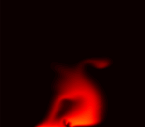
The theory of linear stability analysis of viscosity- and density-driven fingering can provide the instability onset time and the wavenumber versus growth rate relation for the early-time behaviour of the system. The linear analysis, including the non-modal analysis, is valid before the fingers start to interact via nonlinear mechanisms such as tip-splitting, shielding, coalescence, coarsening and channelling, which control plume spreading and mixing. Given our focus on spreading and mixing, we use direct numerical simulations, instead of the linear theory, to resolve such nonlinear interactions and their impact on spreading and mixing metrics. It is important to note that in our numerical model configuration (figure 1), the background flow direction is not parallel with the direction where the effects of gravity are manifested. To the best of the authors’ knowledge, the literature does not provide results from the linear stability analysis that allows for the prediction of instability wave number and growth rate for this specific configuration. Due to the orthogonality of background flow and gravity direction in our configuration, macroscopic vorticity can arise, as visible in figure 2. It is possible to observe in figure 2 that, in the case of a horizontal initial source characterised with multiple density fingers, the faster-moving left-side finger grows downward to reach the bottom boundary while the slower-moving right-side finger grows leftward to merge with the rest of plume at the lower boundary. As a result, the plume appears to roll over itself like a vortex. Merging of viscous fingers is a well-known mechanism (Jha et al. Reference Jha, Cueto-Felgueroso and Juanes2011b, Reference Jha, Cueto-Felgueroso and Juanes2013), but rolling of fingers, as observed in figure 2, due to the interplay between gravitational and viscous fingering mechanisms has not been mentioned in the literature.

Figure 2. Temporal evolution of the solute plume for  $R=3$, $Ra=9000$, $a/b=3$ and $f_L=0.001$. The plume is shown at dimensionless times (a) $t=0.3$, (b) $t=0.6$ and (c) $t=0.9$. These three snapshots in time show the complex nonlinear interplay between viscous and density fingering mechanisms that can lead to folding (e.g. vortex-like structure) of the plume. This observed folding dynamics is unique to the specific model configuration investigated in this work.
3. Numerical implementation
The numerical implementation of our model is similar to that presented in Bonazzi et al. (Reference Bonazzi, Morvillo, Im, Jha and de Barros2021), with the due modifications in the discretised equations to account for the concentration dependence of the solute density. To solve (2.1) numerically for cell-centred pressures, we employ a finite volume method at second-order accuracy (Ferziger, Perić & Street Reference Ferziger, Perić and Street2002). Since (2.1) is expressed in terms of the Darcy flux, i.e. the face-centred flux at the cell interface, we linearise (2.1) using the two-point flux approximation (LeVeque Reference LeVeque2002) of the Darcy flux in (2.2). In this way, we express the flux in terms of the pressure gradient, the concentration distribution and the cell interface transmissibility, which depends on viscosity. The transport problem, governed by (2.6), is solved explicitly for the concentration field,  $c({\boldsymbol {x}},t)$, in terms of the advective and diffusive concentration fluxes computed at the previous time step using a second-order finite difference method.
In our numerical model we use a two-dimensional Cartesian grid where each cell has dimensions  $\Delta x \times \Delta z$, with $\Delta x = 8 \times 10^{-3}$ and $\Delta z = 4 \times 10^{-3}$. The number of cells in both directions, namely $N_x$ and $N_z$, is the same, $N_x=N_z=250$. Thus, the domain lengths in the longitudinal and vertical directions are respectively $L \times H = 2 \times 1$. Our choices for $\Delta x$ and $\Delta z$ are based on a numerical grid resolution analysis that focused on quantities of interest such as the horizontally averaged concentration profile in the vertical direction and the plume's concentration variance, to ensure that the relative percentage error with respect to a more refined grid ( $N_x=N_z=1000$) was below 5 %. The initial source zone in our model is an ellipse with radii $a$ and $b$ in the horizontal and vertical directions, respectively. In our paper, we investigate different ratios $a/b$ (see figure 1 and table 1) in order to explore the effects of the initial plume configuration on transport. Although the ratio $a/b$ is varied, the values of $a$ and $b$ are calculated such that the area of the ellipse, $\mathcal {S}$, at $t_0$ is the same in all the simulations; this way the same mass of solute is initially injected in the domain. For all the ratios explored, we maintain the centre of the ellipse at the dimensionless coordinate ${\boldsymbol {x}_{\boldsymbol {c}}} = (0.3,0.5)$.
Table 1. Model input parameters. All parameter values are dimensionless following the dimensionless groups reported in Appendix A. Parameters R and Ra are varied over a range of values that are uniformly spaced between a minimum value (value on the left of the first colon) and a maximum value (value on the right of the second colon) with a constant increment or spacing between successive values (middle value between the two colons). Here  $R = \ln(\mu_0/\mu_1)$ and Ra is defined in equation (2.7).

4. Comparison with previous work
In this section we compare the results originating from the numerical implementation of the governing equations as described in § 3. We test the performance of the developed numerical simulator using the same physical set-up as reported in the work of Hewitt, Neufeld & Lister (Reference Hewitt, Neufeld and Lister2013). Appendix B provides a brief description of the physical set-up and parameter values used by Hewitt et al. (Reference Hewitt, Neufeld and Lister2013). A relevant difference between our numerical simulation and that in Hewitt et al. (Reference Hewitt, Neufeld and Lister2013) is that we chose a horizontal discretisation with  $\Delta x =(1024)^{-1}$, while in Hewitt et al. (Reference Hewitt, Neufeld and Lister2013) $\Delta x =(2048)^{-1}$. This was done in order to reduce the computational burden of the simulation. Another difference is that the discretisation in the vertical direction is $\Delta z =(250)^{-1}$ in Hewitt et al. (Reference Hewitt, Neufeld and Lister2013), and a vertical coordinate transformation was used to ensure high resolution of the dynamics near the fluid–fluid interface. Here, we opt for a constant vertical discretisation, $\Delta z =(750)^{-1}$. Figure 3(a) shows a comparison between the horizontally averaged concentration profiles obtained from our simulations and those reported by Hewitt et al. (Reference Hewitt, Neufeld and Lister2013) at distinct times. We can see that there is a reasonably good agreement between the two results for the considered times, although some discrepancies are present. Such discrepancies are expected given that the hydrodynamic instability, which causes the fingering behaviour, is triggered in numerical models by the introduction of a small random numerical perturbation which is amplified in time by the physics of hydrodynamic instability and the properties of the numerical method used. Differences in the amplitude and structure of the initial perturbation, which are often unreported in studies, and difference in the accuracy of the numerical discretisation method can also cause differences between studies. Figure 3(b) also illustrates a comparison of the temporal evolution of the horizontally averaged inlet solute mass flux at the top boundary of the domain. As shown in figure 3(b), our computational results are based on a single realisation of the initial perturbation, therefore displaying some noise. The mass flux estimates obtained from Hewitt et al. (Reference Hewitt, Neufeld and Lister2013) are smoother given that they represent an average from multiple realisations of the initial perturbation.

Figure 3. (a) Comparison between the horizontally averaged concentration profiles,  $\bar {c}(z,t)$, of figure 4 in Hewitt et al. (Reference Hewitt, Neufeld and Lister2013) (circles) and those obtained in our simulation (solid line), at three selected times. (b) Comparison between the mass flux $\dot {m}_s$ evolution of figure 5(b) in Hewitt et al. (Reference Hewitt, Neufeld and Lister2013) (dashed line) and that obtained in our simulation (solid line). All quantities are dimensionless in accord with the normalisation provided by Hewitt et al. (Reference Hewitt, Neufeld and Lister2013) and reported in Appendix B.
5. Results and discussion
In this section we perform a series of numerical experiments with the model input parameter values reported in table 1. In § 5.1, we provide a general analysis of the overall behaviour of miscible flow systems for different values of  $R$,
$R$,  $Ra$ and $a/b$, and two different values for the inlet flow rate ( $f_L$). We illustrate how these different parameters impact the solute plume configuration and the corresponding flow field. Section 5.2 analyses how the aforementioned parameters impact specific metrics that quantify mixing and spreading of the plume. Although we have performed simulations for several values of the source zone configuration, we limit our illustrations for the cases of $a/b=1/3$, 1 and 3 for the sake of brevity (simulations were also carried out for $a/b=1/2$ and 2 but are not shown).
5.1. Analysis of flow and transport behaviour
Figure 4 shows the spatial distributions of the concentration field at dimensionless time  $t=1$ from a set of eight representative simulations characterised by distinct values of $R$,
$R$,  $Ra$ and $a/b$. The results displayed in figure 4 correspond to $f_L=0.001$, which we denote here as the low-inlet-flux case. The plumes depicted in figure 4 originate from two different initial source configurations, namely a vertical source ( $a/b=1/3$) and a horizontal source ( $a/b=3$) (see figure 1 for reference). Comparing the plume snapshots in the left- and right-hand columns of figure 4, we observe that the initial plume configuration has a significant impact on the spatial distribution of the solute plume. One of the mechanisms driving this dependency on the initial configuration is gravitational fingering, the strength of which depends on the orientation of the source zone, e.g. compare the plumes obtained for $Ra=9000$ and $R=0$ for both $a/b=1/3$ and 3. Since the gravitational instability grows downward from the plume's interface, a horizontal initial source configuration ( $a/b=3$) provides a longer interface for the gravitational fingers to form and grow. The number of these fingers at early time depends on the typical finger width and the horizontal extent of the source. The typical finger width is a function of $Ra$, as per the linear stability analysis of gravitational fingering (Riaz et al. Reference Riaz, Hesse, Tchelepi and Orr2006), which predicts the finite-size wavelength of initial fingers. This is best shown by comparing the second and third rows in figure 4 for $a/b=3$; an increase in $Ra$ from 1000 to 9000 leads to a decrease in the finger width which means the same interface length can host three fingers instead of one. The case of a vertical initial plume does not provide enough interface length for gravitational fingers to form (i.e. $a/b=1/3$, figure 4a,c,e,g). Higher $Ra$ means sharper plume interface and slower effective diffusion, as visible from comparing the second and third rows.

Figure 4. Concentration fields for the slower inlet flux case,  $f_L=0.001$, at the simulation time $t=1$. (a,c,e,g) Results for the vertical source zone ( $a/b=1/3$) and (b,d, f,h) results for the horizontal source zone ( $a/b=3$). All cases are for a plume heavier than the ambient fluid ( $Ra>0$). (a–d) Cases with low density contrast ( $Ra=1000$) and (e–h) cases with high density contrast ( $Ra=9000$). Ratio $R=3$ implies a less viscous solute compared with the ambient fluid, $R=-3$ implies a more viscous solute and $R=0$ implies no viscosity contrast.
The results depicted in figure 4(a,b) also highlight the effects of  $R>0$ in rapidly diluting the plume via viscous fingering, which (unlike gravitational fingering) does not have a preferential direction. Viscous fingering takes place in both vertical and horizontal directions, and in the case of vertical direction, the effect of viscous fingering superposes on the effect of gravitational fingering, leading to complex plume shapes such as the one shown in figure 4(b). A horizontal initial source under relatively low $Ra$ leads to one gravitational finger growing downward and one viscous finger growing rightward from the plume interface (figure 4b). Due to viscous instability at the tip of the gravitational finger, the finger travels faster and reaches the bottom boundary earlier than $R\leq 0$ cases (second, third and fourth rows). On the other hand, due to gravitational instability, the horizontally travelling viscous finger bends downward. Because of the absence of surface tension effects in a miscible flow, the gravitational and viscous fingers remain connected to the main plume body, which stretches and distorts in a manner reminiscent of chaotic mixing (e.g. Ottino Reference Ottino1989). In essence, the two fingering instabilities interact with each other and our results indicate that the initial source configuration modulates the strength of that interaction.
Figure 4(g,h) shows the combined effects of  $R<0$ and high $Ra$ in hindering mixing. Higher values of density contrast are known to inhibit diffusive mass transfer compared with lower values. For $a/b=3$, gravitational fingering occurs at $R\geq 0$ but is absent at $R=-3$ because at $R=-3$ the velocity magnitude inside the plume is below the threshold for generating the instability; see the velocity field in figure 5(c,d). This important result has been overlooked in some of the prior studies of buoyant mixing that neglect viscosity contrast between the solute and the ambient fluid. When the initial source is vertical or perpendicular to the mean flow direction, i.e. $a/b=1/3$, the low mobility of the plume caused by $R<0$ (see figure 5c,d) retards the sinking of plume caused by $Ra=9000$, thus preventing the solute from reaching the bottom boundary. A close inspection of figure 4(g) for the case of $a/b=1/3$ reveals the emergence of backward-propagating fingers on the rear interface. This occurs because for $R<0$, the rear interface is viscously unstable and the front interface is viscously stable. However, due to the low value of the inlet flux, $f_L=0.001$, the backward-propagating fingers do not grow to become dominant features of the flow.

Figure 5. Maps of the velocity magnitude,  $|{\boldsymbol {v}}|$, at $t=1$ for $f_L=0.001$. Arrow orientation indicates the flow direction and arrow length indicates the magnitude of the velocity vector. The colourbars represent the logarithm of base 10 of the velocity magnitude, $\mathrm {log}_{10}|{\boldsymbol {v}}|$, where the white areas correspond to zones with velocity equal to the mean flow velocity, red-orange areas have velocities faster than the mean and blue areas have velocities slower than the mean. The black line outlines the position of the plume.
Next, we examine the impact of the inlet flux (or the background flux), namely  $f_L$, on both the transport dynamics and the velocity field of the plume. The inlet flux is expected to play a key role in controlling the spreading and mixing behaviour of the plume because it represents a source of mechanical energy directly inserted into the system. We want to investigate how our findings, discussed in figure 4, change when $f_L$ is higher. To investigate this impact, we performed a set of simulations using the same parameter values ( $R$,
$R$,  $Ra$ and $a/b$) for an inlet flux that is ten times higher than that in figure 4, i.e. we increased $f_L$ from 0.001 to 0.01. As a consequence, the mean flow velocity is ten times higher, and we discuss the resulting eight plumes in figure 6 at dimensionless time $t=0.1$ (which corresponds to a tenth of the time considered in figure 4). By doing this, when we compare the results from $t=1$ for $f_L=0.001$ with results from $t=0.1$ for $f_L=0.01$, we are comparing plumes whose centre of mass would be in the same position if no sources of disorder (e.g. viscosity and density contrast) were acting on them.

Figure 6. Concentration field for the faster inlet flux case,  $f_L=0.01$, at $t=0.1$. Analogously to figure 4, results are shown for the (a,c,e,g) vertically and (b,d, f,h) horizontally extended source zones. (a–d) Results for $Ra=1000$ and (e–h) results for $Ra=9000$. (c–f) Results in the absence of viscosity contrast and cases where the solute is (a,b) less and (g,h) more viscous than the ambient fluid.
As illustrated in the first row in figure 6 ( $R=3$ and $Ra=1000$), an increase in the horizontal flow velocity causes viscous fingering to dominate over density-driven fingering (compare figures 4 and 6). We observe that the vertically oriented initial source ( $a/b=1/3$) provides sufficiently long interface for the viscous fingers to nucleate and grow in the downstream direction. The first row of figure 6 reveals that the effect of density becomes limited to the bottom finger, which is thicker, horizontally slower, more concentrated with the denser solute and therefore more prone to sinking toward the bottom boundary; see the corresponding velocity magnitude map in figure 7. When $a/b=3$, the horizontal source orientation does not provide sufficient vertical interface for viscous fingers to form. Hence, at $R=3$, the plume travels as a single finger with high velocity at the finger tip as shown in the kinematic analysis of figure 7. This causes a rapid horizontal stretching of the plume, which triggers gravitational instability on the bottom interface and away from the viscous finger's tip. This is a novel mechanism arising out of interplay between viscosity and density-driven instabilities; viscous fingering triggers density fingering. However, they dominate different parts of the plume, which are determined by the velocity field. The initial shape of the source (horizontal versus vertical) modulates the strength of the interplay; a horizontal source ( $a/b=3$) enhances the effect of gravity fingering compared to a vertical source ( $a/b=1/3$). This is further supported by the kinematic analysis associated with figure 7.

Figure 7. Maps of the velocity magnitude,  $|{\boldsymbol {v}}|$, at $t=0.1$, for $f_L=0.01$. Arrow orientation indicates the flow direction and arrow length indicates the magnitude of the velocity vector. The colourbars represent the logarithm of base 10 of the velocity magnitude, i.e. $\mathrm {log}_{10}|{\boldsymbol {v}}|$, where the white areas correspond to zones with velocity equal to the mean flow velocity, red-orange areas indicate velocities faster than the mean and blue areas indicate velocities slower than the mean. The black line outlines the position of the plume.
The second and third rows of figure 6 show the solute plumes in the absence of viscosity contrast ( $R=0$). We observe that an increase in the mean flow velocity, which is horizontally oriented in our study, significantly decreases the effect of density contrast on mixing even in the absence of viscous fingering. An increase in $Ra$ from $1000$ to $9000$ (figures 6c,d and 6e,f, respectively) does not affect the shape of the plume or, more importantly, the degree of mixing (as seen from the colour scale of the two plumes), for neither $a/b=1/3$ nor $a/b=3$. The flow is predominantly advective due to the higher inlet flux; compare figures 4 and 6.
When  $R<0$ (bottom row in figure 6), we observe that a larger value of $f_L$ impacts the competition between viscous and gravitational fingering; compare with the bottom row of figure 4. The results in figure 6 show that viscous fingering becomes dominant over density-driven fingering at a higher inlet flux $f_L$. For $a/b=1/3$, the initial source orientation paired with the increased horizontal velocity allows the growth of the backward viscous fingers that could not grow for the same values of $R$,
$R$,  $Ra$ and $a/b$ in figure 4. As depicted in figure 7(c,d) for $R<0$, the low velocity magnitude inside the plume affects the mixing behaviour also in the case for $a/b=3$, when viscous fingers are not present due to the source orientation. In this case, the low mobility of the plume prevents it from travelling with the mean flow, thus obstructing spreading. The plume shape resembles the shape of the plumes observed for the cases with $R=0$; however, it is asymmetric between downstream and upstream edges of the plume due to the viscosity contrast between the two fluids. A ‘wake’ emerges downstream of the plume reminiscent of turbulent flow around a cavity or a bluff body (Wu Reference Wu1972). This effect, paired with a high $Ra$ that hinders diffusion, causes the plume to be poorly mixed with the ambient fluid.
5.2. Mixing and spreading
5.2.1. Fluid interface dynamics
We are interested in relating the plume's interface to the concentration spatial variance for different initial plume configurations. The concentration variance  $\sigma ^2_c$ can be viewed as a plume mixing indicator (e.g. Boso et al. Reference Boso, de Barros, Fiori and Bellin2013; Bonazzi et al. Reference Bonazzi, Dentz and de Barros2022). The concentration spatial variance is defined as
 \begin{equation} \sigma^2_c(t) = \frac{1}{\varOmega(t)} \int_{\varOmega(t)}\left[c(\boldsymbol{x},t)-\langle c(\boldsymbol{x},t)\rangle \right]^2 \,\mathrm{d}\varOmega, \end{equation}
where  $\varOmega (t)$ is the area occupied by the solute plume at time $t$. It is defined as the area where concentration is higher than a threshold value $c_i$, with $c_i=10^{-3}$, and $\langle c({\boldsymbol {x}},t)\rangle$ is the plume's spatial mean concentration, defined as
 \begin{equation} \langle c(\boldsymbol{x},t) \rangle = \frac{1}{\varOmega(t)} \int_{\varOmega(t)}c(\boldsymbol{x},t) \,\mathrm{d}\varOmega. \end{equation}
Since the solute is neither injected nor withdrawn from the domain during the time period of analysis, we can obtain the evolution equation of  $\sigma _c^2$ from the advection–dispersion equation (2.6) following the steps described in Jha et al. (Reference Jha, Cueto-Felgueroso and Juanes2011b):
 \begin{equation} \frac{{\rm d}\sigma_c^2}{{\rm d}t}={-}2\langle \epsilon \rangle, \end{equation}
which implies  $\sigma _c^2$ decreases and mixing increases monotonically with time for all parameter values studied here and the rate at which concentration variance decreases is proportional to the mean scalar dissipation rate $\langle \epsilon \rangle$.
To better quantify the effect of shape of the initial source on mixing and spreading, we define a plume shape metric  $\eta$ as follows:
 \begin{equation} \eta(t)=\frac{\hat{\eta}(t)}{\eta_o}, \end{equation}
where  $\hat {\eta }$ is calculated as
 \begin{equation} \hat{\eta}(t)=\frac{\ell_{c_i}(t)}{\mathcal{A}_{c_i}(t)}, \end{equation}
where  $\ell _{c_i}$ is the length of the isoline of concentration $c=c_i$, and $\mathcal {A}_{c_i}$ is the area of the plume delimited by such an isoline. In this study, we set $c_i = 1 \times 10^{-3}$. We normalise $\hat {\eta }$ by its initial value given by $\eta _o \equiv \hat {\eta }(t_0)= (\ell _{c_i}/\mathcal {A}_{c_i})|_{t=t_0}$.
The shape metric  $\eta$ is defined to account for the length of the interface between the solute plume and the ambient fluid, and for the area occupied by the plume. Since the interface is where mixing happens, and the plume area is related to spreading, the definition of $\eta$ includes mechanisms of both mixing and spreading. For diffusion-dominated transport of an isotropic (circular) source, e.g. $R=0$, $Ra \leq 1000$ and $a/b=1$, the plume radius increases proportionally to $\sqrt {t}$, the plume interface is $\ell _{c_i} \propto \sqrt {t}$ and the area is $\mathcal {A}_{c_i} \propto t$ (Jha et al. Reference Jha, Cueto-Felgueroso and Juanes2011a), rendering $\eta \propto t^{-1/2}$, i.e. $\eta$ decreases monotonically in time during diffusive transports. For diffusive systems, $\sigma _c^2$ also decays with time such that $\eta \propto \sigma _c^2$, with the proportionality factor given by the initial source shape. In convection-dominated transports due to viscous fingering or permeability heterogeneity, $\eta$ can increase at early time due to rapid stretching of the plume interface while the plume area stays relatively constant or grows slower than the interface length. This would imply that mixing is still in its early stages ( $\sigma _c^2$ is relatively high) and the solute has not mixed with the ambient fluid enough to occupy an area significantly larger than the initial one, but mixing will increase rapidly in the future across the stretched interface as implied by high $\eta$. As time progresses and the solute becomes more mixed with the ambient fluid, we expect $\eta$ to decrease as the area of the plume increases and its interface becomes less sinuous. The result is that $\eta$ evolves non-monotonically in convective systems.
Since the concentration spatial variance  $\sigma _c^2$ quantifies the degree of mixing (high $\sigma _c^2$ means lack of mixing; see Bonazzi et al. Reference Bonazzi, Morvillo, Im, Jha and de Barros2021), we analyse the co-evolution of $\eta$ and $\sigma _c^2$ in figures 8 and 9 to learn how the interplay of viscous and gravitational fingering affects spreading and mixing of plumes of different initial shapes. In the sense of nonlinear dynamical systems, the $\eta$ versus $\sigma _c^2$ plot can be seen as a phase space diagram for investigating the effect of fingering and shape parameters on mixing. This is equivalent to $\sigma _c^2$ versus $\langle \epsilon \rangle$ phase diagram in viscous fingering (Jha Reference Jha2014). We first analyse the evolution behaviour for a diffusive system, i.e. $[R,Ra]=[0,1000]$, to set a baseline for interpreting these plots. For a diffusive system, both $\eta$ and $\sigma ^2_c$ decrease monotonically in time, which can be inferred from figures 8 and 9 by noting that darker shades denote early time and lighter shades denote late times. Therefore, the $\eta$ versus $\sigma _c^2$ trend is also monotonic and agrees with our previously mentioned hypothesis for diffusive transport of a circular source. The effect of vertical or horizontal initial shape on the $\eta$ versus $\sigma _c^2$ trend is minimal in diffusive systems except in the presence of boundary condition effects; the vertical source ( $a/b=1/3$) at slower mean flow ( $f_L=0.001$) reaches the bottom boundary fast and experiences the effect of no-flux boundary condition, which causes a rapid drop in $\eta$. At higher flux $f_L=0.01$ (figure 9), this effect is absent and we recover the baseline trend in $\eta$ versus $\sigma _c^2$. In convective systems with fingering instabilities, $\eta$ behaves nonlinearly with $\sigma _c^2$ because of significant changes in the plume shape, e.g. horizontal viscous fingering in figure 9 for $[R,Ra,a/b]=[3, 1000, 3]$.

Figure 8. Scatterplots of the solute plume's  $\eta$ and $\sigma ^2_c$ for $f_L=0.001$ at ten equidistributed time intervals between $t=0.1$ (dark colour shade) and $t=1$ (light colour shade). Results for $Ra=1000$ (a–c) and $Ra=9000$ (d–f), and for $R=-3,0$ and $3$ (left, centre and right columns, respectively).

Figure 9. Scatterplots of the solute plume's  $\eta$ and $\sigma ^2_c$ for $f_L=0.01$ at equidistributed time intervals between $t=0.025$ (dark colour shade) and $t=0.5$ (light colour shade), or until the time the plume reaches the right-hand boundary of the domain. Results for $Ra=1000$ (a–c) and $Ra=9000$ (d–f), and for $R=-3,0$ and $3$ (left, centre and right columns, respectively).
The effect of  $R$ on plume shape ( $\eta$) and mixing ( $\sigma _c^2$) metrics is amplified when convection dominates the flow, which happens at higher $Ra$ (second row in figure 8) and higher $f_L$ (both rows in figure 9). When both density- and viscosity-driven fingering occurs, their effects are superposed on the baseline diffusive trend, rendering the $\eta$ versus $\sigma ^2_c$ trend complex. In these cases, the initial source shape ( $a/b$) plays a more important role in determining the $\eta$ versus $\sigma ^2_c$ trend than in the cases where fingering is absent.
The importance of relating an indicator of mixing, such as  $\sigma ^2_c$, to a plume shape metric, such as $\eta$, stems from the observation that mixing is more intense where the concentration gradients are higher, i.e. at the interface between an injected solute and the ambient fluid. Engineers and hydrogeologists who may need to maximise or minimise mixing between two fluids can attempt to control the plume shape evolution in time by leaning towards one initial solute source orientation or another. For example, if a fluid is being injected in an aquifer for the purpose of groundwater remediation, it is desirable to ensure maximum mixing between the two fluids. Traditionally, this implies that the remediation fluid selection and its injection are designed in a way to maximise the interface between the two fluids; in other words, a high $\eta$ has been traditionally associated with good mixing, or low values of $\sigma ^2_c$. We have shown in figures 8 and 9 that, depending on several factors (the mean flow velocity, the initial shape and orientation of the injected solute source and the degree of viscosity and density contrast between the two fluids), the same degree of mixing can be achieved for different values of the shape parameter $\eta$, that is, for different shapes of the solute plume. Similarly, the same value of $\eta$ can be associated with different degrees of mixing; see, for example, cases for $R=-3$ and $Ra=9000$ in figure 9 for $a/b=3$ and $a/b=1/3$.
5.2.2. Mixing analysis in the  $R$–$Ra$ parameter space and concentration statistics


To understand how mixing evolves globally in the domain as a function of the density and viscosity contrasts, we plot the spatially averaged mean  $\langle c \rangle$ and variance $\sigma ^2_c$ of the concentration field as contour maps in the parameter space of $R$ and $Ra$ for $f_L=0.001$ and $f_L=0.01$ and distinct values for $a/b$ (see figures 10 and 11, respectively). The spatial statistics of the concentration field can be viewed as global measures of mixing. As discussed in Bonazzi et al. (Reference Bonazzi, Dentz and de Barros2022), the spatial mean concentration is related to the dilution index (Kitanidis Reference Kitanidis1994) and therefore can be used as a descriptor for the global mixing state of a solute plume. Similarly, the concentration variance is related to the global scalar dissipation rate (Kapoor & Gelhar Reference Kapoor and Gelhar1994). Both figures present results for three different values of the initial solute source shape ( $a/b=1/3$, 1 and 3), presenting the contour maps for the concentration spatial mean (top row of figures 10 and 11) and variance (bottom row of figures 10 and 11). Results for $\langle c \rangle$ and $\sigma ^2_c$ are shown at time snapshots $t=1$ (figure 10) and $t=0.1$ (figure 11).

Figure 10. Contour plots of the spatial statistics of the concentration. The mean concentration (a–c) and concentration variance (d–f) of the plume at  $t=1$ for $f_L=0.001$ and for the range of $R$ and $Ra$ investigated for different initial shapes: $a/b=1/3$, 1 and 3.

Figure 11. Contour plots of the spatial statistics of the concentration. The mean concentration (a–c) and concentration variance (d–f) of the plume at  $t=0.1$ for $f_L=0.01$ and for the range of $R$ and $Ra$ investigated for $a/b=1/3$, 1 and 3.
Focusing on the low-inlet-flux case reported in figure 10, we can see that, for  $R<0$, a vertical initial source ( $a/b=1/3$, left column) leads to better mixing compared to a horizontal source, in agreement with the analysis carried out for the bottom row images in figure 4. For $R>0$, however, a better degree of global mixing (lower $\langle c \rangle$ and $\sigma ^2_c$) is achieved for $a/b=3$ because the horizontal initial source facilitates the creation of gravity fingers along with viscous fingers. For $R \approx 0$, values of $\langle c \rangle$ and $\sigma ^2_c$ lie between those computed for $R>0$ and $R<0$. We also observe that if $a/b=1/3$, the impact of viscosity contrast between the fluids on the resulting concentration spatial mean and variance is not as strong as in the case of $a/b=3$, in which the difference between the upper and the lower part of the parameter space is more noticeable. In regard to the effect of $Ra$, the results in figure 10 show that for a fixed $R$, better mixing is achieved for lower values of $Ra$. This is due to the fact that high density contrasts lead to less diffusive mass transfer. However, the impact of $Ra$ on mixing becomes almost negligible for $R>0$: note how on the upper half of the parameter spaces in figure 10, the concentration isolines are almost horizontal. A similar isoline orientation is found for $R<0$ when $Ra \gtrsim 6000$, suggesting that as $Ra$ increases its impact on mixing tends to ‘stabilise’. The reason is that reduction in mixing due to lower diffusion at higher $Ra$ is balanced by increase in mixing due to a longer interface at higher $Ra$; a similar observation has been made for fluid mixing from viscous fingering (Jha et al. Reference Jha, Cueto-Felgueroso and Juanes2011a). Further investigation involving a broader range of $Ra$ considered would be warranted to support this hypothesis. As expected, the impact of $Ra$ on mixing is higher for $a/b=3$ because a horizontally oriented initial source allows gravitational fingering.
Next, we analyse figure 11 to understand how the physics of mixing changes when the inlet flux is increased tenfold ( $f_L=0.01$). The observation that a vertically extended initial source translates to better mixing, compared with a horizontal source, for $R<0$ is still valid. However, unlike what was observed in figure 10, when the mean flow velocity increases, for $R>0$, a plume originating from a horizontally extended initial source ( $a/b=3$) does not correspond to the best mixed scenario. Since a higher flow velocity means that viscous fingers are clearly forming in the direction of flow, $a/b=1/3$ (perpendicular to the flow direction) is the shape that offers more interface and favours finger formation. As seen in figure 6, for $R>0$ and $a/b=3$, the plume travels as a single finger, which inhibits convective mixing. Another difference in regard to the discussion of figure 10 is that in figure 11, values of $R \approx 0$ do not result in a mean concentration that lies between those observed for $R>0$ and $R<0$. For $R \approx 0$ we have the highest computed values of $\langle c \rangle$, and this trend is exacerbated for $a/b=3$. The reason is that a high $f_L$ value enhances viscous fingering of the vertical source, forward fingering for $R>0$ and backward fingering for $R<0$. Fingering-induced mixing leads to a drop in $\langle c \rangle$. Fingering is absent at $R \approx 0$, and hence we observe highest $\langle c \rangle$ values at $R \approx 0$. As mentioned previously, at $R=0$, mixing is not significantly affected by the density contrast, whose effect on solute transport is being hampered by the higher mean flow velocity. The solute plume travels along the mean flow direction almost undisturbed. On the other hand, the lower velocity inside the plume due to $R<0$ causes downstream stretching of the plume and appearance of the previously mentioned ‘wake’ (see § 5.1, discussion for figure 6), thus resulting in a mean concentration lower than that computed with $R=0$. The difference in $\langle c \rangle$ between $R=0$ and $R<0$ is not as large as that between $R=0$ and $R>0$, where the formation of a single finger that travels faster than the mean flow velocity is sufficient to achieve the best degree of mixing among the ones obtained for $a/b=3$.
The effect of  $Ra$ on both $\langle c \rangle$ and $\sigma _c^2$ is almost negligible for $R>0$, similar to what was observed in figure 10. Recall that these observations are at a specific time step; $Ra$ does influence the time evolution of mixing, e.g. the evolution of $\eta$ in figure 9. If $a/b=1/3$, density contrast does not seem to have a significant impact on the mixing metrics considered here for any value of $R$. For $a/b=3$ on the other hand, if $R<0$, we observe again that density differences between the fluids seem to have an impact only for $Ra \lesssim 6000$, analogous to the case of lower $f_L$ in figure 10.
6. Effects of heterogeneity in the permeability field
Next, we focus on quantifying the effect of permeability heterogeneity on plume mixing and spreading under hydrodynamic instabilities. In order to account for heterogeneity, we consider a stratified porous medium. Stratification or layering is a common feature in many geophysical flows. For example, a layered geological formation leads to depth dependence in hydraulic properties, e.g. causing the permeability to change significantly from a clean sandstone layer of high permeability to an adjacent silty sandstone layer of low permeability. This is relevant for solute transport because it is expected that the solute plume will move faster and farther in a high-permeability layer compared with a low-permeability layer. Therefore, it is intuitive to expect enhanced plume stretching, sharper concentration gradients along the stretched interface and faster mixing across the fluid interface. We model stratification following the model described in (2.9) in Nijjer et al. (Reference Nijjer, Hewitt and Neufeld2019):
 \begin{equation} \mathrm{ln}(k) ={-}\sigma^2_{st} \cos(2{\rm \pi} nz) -\mathrm{ln}(\mathrm{I}_{0}(\sigma^2_{st})), \end{equation}
where  $\sigma ^2_{st}$ is the log-permeability variance, $z$ is the vertical coordinate, ${\rm I}_0$ is the modified Bessel function of the first kind and $n$ is the wavenumber which determines the length scale of the permeability variations. In this study, we set $n=2$, thus obtaining four layers in the domain. We simulate transport for two different values of the log-permeability variance: $\sigma ^2_{st}=0.05$ and $\sigma ^2_{st}=0.1$, with the same average permeability value. We also consider the baseline case of a homogeneous medium ( $\sigma ^2_{st}=0$) with a uniform permeability value equal to the average permeability in the heterogeneous cases. Regarding fluid properties, we set $R=2$ (the plume is less viscous than the ambient fluid) and $Ra=5000$ (the plume is denser than the ambient fluid). We also present results for $R=0$ for comparison. For the upcoming results, we set the inlet flux parameter to $f_L=0.01$ and consider two values of the initial source configuration: $a/b=1/3$ (vertical orientation) and $a/b=3$ (horizontal orientation).
Figure 12 shows the concentration fields for different levels of heterogeneity and values of  $R$. Results are depicted at dimensionless time $t=0.1$ for $a/b=1/3$. Increasing heterogeneity in a stratified medium results in the formation of preferential flow paths in higher-permeability layers. As $\sigma ^2_{st}$ increases, the middle layer becomes more permeable, which causes additional stretching of the plume as seen in figure 12. The presence of heterogeneity changes the location of the peak concentration in the plume. For a homogeneous case ( $\sigma ^2_{st}=0$), highest concentration is at the bottom of the plume because of gravitational sinking ( $Ra=5000$). For layered cases, the highest concentration occurs in the high-permeability middle layer. This occurs with or without the viscosity contrast; however, viscous fingering at $R=2$ creates additional mechanisms that are superposed on the effects due to density contrast and layering. We know from the literature (Sajjadi & Azaiez Reference Sajjadi and Azaiez2013; Nicolaides et al. Reference Nicolaides, Jha, Cueto-Felgueroso and Juanes2015; Nijjer et al. Reference Nijjer, Hewitt and Neufeld2019; Bonazzi et al. Reference Bonazzi, Morvillo, Im, Jha and de Barros2021) that viscous fingering interacts with permeability heterogeneity. For example, during continuous slug injection in layered media (Nijjer et al. Reference Nijjer, Hewitt and Neufeld2019), viscous fingering dominates the mixing behaviour at early times, and when the fingers have grown to become comparable to the layer thickness scale, heterogeneity begins to dominate mixing. Such investigations of the interplay between fingering and heterogeneity mechanisms are missing for finite-size solute bodies, which we address here (see figures 12 and 13). The high flow velocity in the middle layer (figure 12e) causes tip splitting of the fingers followed by tip blunting, which we explained in our prior work; see figure 3 in Bonazzi et al. (Reference Bonazzi, Morvillo, Im, Jha and de Barros2021). The result of these interactions is rapid mixing in the high-permeability middle layer. At $R=0$, these effects are absent, and high concentrations in the middle layer persist for a longer duration.

Figure 12. Concentration fields at  $t=0.1$ for $a/b=1/3$, for three different levels of heterogeneity: (a,b) no heterogeneity ( $\sigma ^2_{st}=0$), (c,d) $\sigma ^2_{st}=0.05$ and (e,f) $\sigma ^2_{st}=0.1$. (a,c,e) Results for $R=2$ and (b,d, f) the corresponding cases in the absence of viscosity contrast ( $R=0$). All results are for $Ra=5000$ and $f_L=0.01$. The permeability field has been superimposed in transparency to the concentration fields; light shades correspond to higher-permeability layers, while darker shades to low-permeability ones.

Figure 13. Maps of the velocity magnitude,  $|{\boldsymbol {v}}|$, at $t=0.1$ for $f_L=0.01$ and $a/b=1/3$. The arrows indicate the velocity vector with both direction and magnitude information. The colourbars represent the logarithm of velocity magnitude, i.e. $\mathrm {log}_{10}|{\boldsymbol {v}}|$. The black line outlines the position of the plume. All results are for $Ra=5000$.
When the initial solute source is horizontally oriented ( $a/b=3$, figure 14), permeability stratification does not have a significant impact on solute transport in absence of viscous fingering ( $R=0$, figure 14b,d, f). This is because the source zone is not crossing multiple layers at the considered time. However, when viscosity contrast is present ( $R=2$, figure 14a,c,e), stratification favours the formation of viscous fingers in the horizontal direction, a feature that was not observed for analogous cases in homogeneous media discussed in § 5. The horizontal finger formation can be explained by observing figure 15(a,c,e). As the difference in velocity magnitude between layers increases, the upper and lower edges of the plume experience lower velocity magnitudes compared with the centre. The horizontal direction of the velocity field causes the centre of the plume to travel faster than its edges and split into two fingers, following the tip splitting mechanism. At $\sigma ^2_{st}=0.05$ (figure 15c), the upper finger eventually merges into the dominating lower finger, following the finger coarsening mechanism (Jha et al. Reference Jha, Cueto-Felgueroso and Juanes2011b). At $\sigma ^2_{st}=0.1$, heterogeneity is strong enough to sustain the growth of both fingers for a longer time (figure 14e). Eventually, the fingers will merge as in the case of a vertically oriented source ( $a/b=1/3$), and permeability heterogeneity will be the dominant agent affecting solute mixing and transport.

Figure 14. Concentration fields for  $a/b=3$ at $t=0.1$ for three levels of heterogeneity: (a,b) $\sigma ^2_{st}=0$ (no heterogeneity), (c,d) $\sigma ^2_{st}=0.05$ and (e, f) $\sigma ^2_{st}=0.1$. All results are for $Ra=5000$ and $f_L=0.01$.

Figure 15. Maps of the velocity magnitude,  $|{\boldsymbol {v}}|$, for $a/b=3$ at $t=0.1$ for $f_L=0.01$. The arrows indicate the velocity vector with both direction and magnitude information. The colourbars represent the logarithm of velocity magnitude, i.e. $\mathrm {log}_{10}|{\boldsymbol {v}}|$. The black line outlines the position of the plume. All results are for $Ra=5000$.
In this section, the layer thickness is comparable to the size of the initial source. The horizontally oriented source is inside the higher-permeability layer, i.e. the permeability values in that layer (albeit not constant due to the sinusoidal nature of the field) are higher compared with the mean permeability. However, we can see that even such slight variation of the permeability is able to affect the transport behaviour. This suggests that the structure of the permeability field might impact the interplay between density and viscosity contrast in driving mixing. If the permeability field structure is reversed (i.e. switching the locations of high-permeability layers with the locations of the low-permeability layers), or if the solute injection is located between layers, the impact of the structure of the permeability field on mixing might be different.
7. Summary
The need for modelling the effects of viscosity and density contrasts in the spreading and mixing dynamics of a solute body has been recognised and addressed in the literature given its importance in contaminant transport, energy recovery and storage in the subsurface environment. In all these applications, solutes are characterised by viscosity and density values that differ from those of the ambient fluid. Furthermore, these solutes are injected into the subsurface through source zones of different spatial configurations. Our work focuses on systematically investigating the impact of the initial configuration of the source zone on the transport behaviour in the presence of hydrodynamic instabilities. The numerical analysis carried out in the present work illustrates the importance of both the initial solute source configuration and the intensity of the inlet (background) flux in controlling the relative significance of  $R$ and $Ra$ in the mixing and spreading behaviour. In the following, we highlight the key findings of our analysis.
Effect of viscosity contrast on mixing: For a homogeneous medium and low inlet or background flux, gravitational fingering is impeded when the solute is more viscous than the ambient fluid, i.e.  $R<0$. When $R>0$, viscous fingering occurs in both horizontal and vertical directions and in the latter case, viscous fingering and gravitational fingering effects overlap. For $R<0$, better mixing is achieved with a vertically oriented initial source. If more mixing is desired under $R>0$ conditions, a horizontally oriented solute source is preferable at a low background flux, whereas a vertical source is preferable at high background flux. At higher inlet flux, when $R>0$, a horizontally oriented source does not result in the best degree of mixing because the dominance of viscous fingering (as the primary driver of mixing) allows a vertically extended source to form a larger number of fingers. The importance of viscosity contrast in enhancing mixing when the inlet flux is higher means that the degree of mixing is lower when no viscosity contrast is present ( $R\approx 0$).
Effect of density contrast on mixing: For a homogeneous medium and low inlet flux, higher values of  $Ra$ were also found to allow lower rates of diffusive mass transfer. The impact of $Ra$ on mixing was found to be almost negligible when $R>0$. A horizontally oriented initial source zone allows gravitational fingers to form and grow in the vertical direction. The number of fingers increases with $Ra$ in accordance with the linear stability analysis theory. At higher inlet flux, the role of $Ra$ in mixing is minor for a vertically oriented source for any value of $R$ considered. For a horizontally oriented source, $Ra$ appears to affect mixing when $R<0$.
Effect of background flow velocity on mixing: We established that a higher mean flow velocity hampers gravitational fingering, thus rendering viscous fingering the dominant force driving mixing. As a consequence, the source orientation becomes a significant factor when  $R<0$. Under these conditions, we observed the following: (1) for $a/b=1/3$ (vertically oriented source), a higher flow velocity allows the formation of viscous fingers, which will lead to enhanced mixing; while (2) for $a/b=3$ (horizontally oriented source) the absence of viscous fingering and the low velocity inside the plume result in poor mixing.
Relationship between mixing and plume shape: The numerical analysis presented here allowed us to investigate the relationship between the degree of mixing and the length of the interface between the solute and the ambient fluid (i.e. plume shape). Traditionally, one would expect enhanced mixing rates for increased elongation of the plume's interface with the surrounding fluid. In the context of aquifer remediation, hydrologists and engineers aim to maximise the interface between the contaminant and groundwater in order to enhance dilution and reaction rates (e.g. Bagtzoglou & Oates Reference Bagtzoglou and Oates2007; Kitanidis & McCarty Reference Kitanidis and McCarty2012; Trefry et al. Reference Trefry, Lester, Metcalfe, Ord and Regenauer-Lieb2012; Piscopo, Neupauer & Mays Reference Piscopo, Neupauer and Mays2013). As shown in § 5.2.1, the relationship between mixing and plume shape is non-trivial when fingering instabilities are present. The results in § 5.2.1 shed novel insights on the role of source orientation, inlet flux and fingering instabilities (i.e. viscosity and density contrasts) in controlling the plume shape and its mixing dynamics. Our results show that the same degree of mixing can be achieved for different plume shapes.
Effect of permeability heterogeneity on mixing: To account for the heterogeneity, we considered a stratified permeability field. We found that, for a vertically oriented solute source, heterogeneity in the porous medium affects the location of the plume's highest concentration values by overlaying the effect of gravitational instability and favouring higher concentration values in the higher-permeability layer. The high flow velocity in the more permeable layer causes tip splitting and results in rapid mixing. For a horizontally oriented solute source, the combined effect of viscosity contrast and permeability heterogeneity results in fingering along the flow direction, a result not observed for the homogeneous media analysis presented in § 5.
The simulations carried out in this work highlight the importance of the initial solute source configuration and the intensity of the inlet flux in modulating both the plume's spreading and mixing behaviour in homogeneous and heterogeneous permeability fields. Additional research is needed to understand these complex interactions in three-dimensional settings, larger computational domains, in the absence of interaction with the bottom boundary of the domain, with different injection modes and distinct conceptualisations of the permeability field, including higher levels of permeability heterogeneity.
Acknowledgements
The authors would like to thank all the reviewers and the Editor for the constructive comments that helped improve the overall quality of this work.
Funding
The authors acknowledge the support from US National Science Foundation Grant 2025285.
Declaration of interests
The authors report no conflict of interest.
Appendix A
The governing dimensional equation for the flow field is given by
 \begin{equation} \boldsymbol{\nabla}\boldsymbol{\cdot} \boldsymbol{\hat{q}}(\boldsymbol{\hat{x}},\hat{t}) = 0, \end{equation}
where the  $(\hat {\cdot})$ symbol denotes a dimensional variable and $\boldsymbol {\hat {q}}$ is the specific discharge defined by Darcy's law as
 \begin{equation} \boldsymbol{\hat{q}}(\boldsymbol{\hat{x}},\hat{t}) ={-} \frac{\hat{k}(\boldsymbol{\hat{x}})}{\hat{\mu}(\hat{c}(\boldsymbol{\hat{x}},\hat{t}))} (\boldsymbol{\nabla} \hat{p}(\boldsymbol{\hat{x}},\hat{t})-\Delta \rho g \mathcal{F}(\hat{c}(\boldsymbol{\hat{x}},\hat{t})). \end{equation}
The dimensional governing equation for transport of an inert solute is
 \begin{equation} \phi \frac{\partial \hat{c}(\boldsymbol{\hat{x}},\hat{t}) }{\partial \hat{t}} + \boldsymbol{\hat{q}}(\boldsymbol{\hat{x}},\hat{t}) \boldsymbol{\cdot} \boldsymbol{\nabla} \hat{c}(\boldsymbol{\hat{x}},\hat{t}) = \phi D \nabla^2 \hat{c}(\boldsymbol{\hat{x}},\hat{t}). \end{equation}
 In a homogeneous field,  $\hat {k}(\boldsymbol {\hat {x}})$ in (A2) is a constant, $\hat {k}(\boldsymbol {\hat {x}})=\hat {k}$, with corresponding dimensionless group $k = \hat {k}/k_c$, with $k_c=\hat {k}$. We then define the following dimensionless groups:
 \begin{equation} \boldsymbol{x} = \frac{\boldsymbol{\hat{x}}}{\ell}; \quad\boldsymbol{q} = \frac{\boldsymbol{\hat{q}}}{Q}; \quad\boldsymbol{t} = \frac{\boldsymbol{\hat{t}}}{\tau} ; \quad c= \frac{\hat{c}}{c_o}; \quad\mu = \frac{\hat{\mu}}{\mu_1}; \quad p = \frac{\hat{p}}{p_c}, \end{equation}
where  $\ell$ represents the characteristic length of the domain (chosen to be its thickness); $Q$ denotes the characteristic velocity defined as $Q=k_c\Delta \rho g/ \mu _1$; $\tau$ corresponds to the characteristic time scale defined as $\tau =\mu _1 \ell \phi / k_c \Delta \rho g$; $p_c$ is the characteristic pressure defined as $p_c = \ell \Delta \rho g$; $c_o$ is the injected solute initial concentration; and $\mu _1$ is the viscosity of the injected solute. By substituting (A4a–f) into (A1)–(A3), we find the corresponding dimensionless equations in § 2, (2.1), (2.2) and (2.6).
In a heterogeneous field, the dimensionless form of the governing equations for flow and transport will remain the same as presented in (2.1) and (2.6), respectively; however, permeability will not disappear from the dimensionless form of Darcy's law:
 \begin{equation} \boldsymbol{q}(\boldsymbol{x},t) ={-} \frac{k(\boldsymbol{x})}{\mu(c(\boldsymbol{x},t))} [\boldsymbol{\nabla} p(\boldsymbol{x},t) - c(\boldsymbol{x},t)\boldsymbol{e}_z ]. \end{equation}
Appendix B
We test our numerical simulator by comparing its result for a fixed interface case with the result for the same case from Hewitt et al. (Reference Hewitt, Neufeld and Lister2013). The set-up for this case consists of a zero mass and buoyancy fluxes condition at the bottom and side boundaries, while the upper boundary has zero vertical velocity and a constant concentration  $C^*_m$ imposed. The initial concentration $C^*_{-}$ in the porous medium is constant with $C^*_{-}< C^*_m$, so that as time evolves the dimensional concentration $C^*$ is $C^*_{-}< C^*< C^*_m$. In Hewitt et al. (Reference Hewitt, Neufeld and Lister2013) the dimensionless concentration $C$ is defined in such a way that $-1< C<0$. We rescaled it in our verification process so that $0< C<1$.
Times are normalised with the convective time scale  $T$, with $T=\phi H/U$. Lengths are normalised with the initial interfacial height $H$, which in the examined case corresponds to the domain thickness. Parameter $U$ is the convective velocity scale, $U= k \Delta \rho g/ \mu$, analogous to $Q$ in Appendix A with the notable difference that in Hewitt et al. (Reference Hewitt, Neufeld and Lister2013) the system viscosity $\mu$ is a constant. Pressures are normalised with the characteristic pressure $p_c=\mu U H/k$. Further details about the process to obtain the dimensionless governing equations can be found in § 3.2 of Hewitt et al. (Reference Hewitt, Neufeld and Lister2013).
A comparison between the concentration fields in Hewitt et al. (Reference Hewitt, Neufeld and Lister2013) and that obtained in our numerical simulation at  $t=4$ is presented in figure 16. Differences between the two images are due to the nature of the random perturbation at the top boundary, to the different horizontal grid resolution ( $\Delta x =(1024)^{-1}$ in our study, and $\Delta x =(2048)^{-1}$ in Hewitt et al. (Reference Hewitt, Neufeld and Lister2013)) and to the slight differences in the image colour scale.

Figure 16. Comparison between the concentration field at  $t=4$ from figure 4(a) in Hewitt et al. (Reference Hewitt, Neufeld and Lister2013) (a) and the concentration field obtained with our model at the same time (b).


 Open access