


1. Introduction
The accurate description of the strong non-equilibrium region inside a shock has remained an elusive problem in theoretical fluid dynamics. The variation of macroscopic properties across this narrow region (of the order of a few mean free paths) is quite steep and the well-known Navier–Stokes equations based on the small gradient approximation are found to be inadequate (Becker Reference Becker1929; Thomas Reference Thomas1944; Gilbarg Reference Gilbarg1951; Gilbarg & Paolucci Reference Gilbarg and Paolucci1953). The Mach number ( $Ma$) and the Knudsen number ( $Kn$) are two important non-dimensional numbers that characterize the shock profiles. The Mach number is defined as the ratio of velocity of the shock and the adiabatic sound velocity, both defined at the upstream point, and is greater than unity. The Knudsen number measures the degree of rarefaction and is defined as ratio of the mean free path and the characteristic length scale. In a typical shock wave, the Knudsen number is of the order of unity and falls in the transition regime. With no physical wall boundaries and well-defined boundary conditions, the one-dimensional normal shock has served as a benchmark problem for assessing the accuracy of continuum theories, along with the force-driven Poiseuille flow problem (Tij & Santos Reference Tij and Santos1994; Uribe & Garcia Reference Uribe and Garcia1999; Jadhav, Singh & Agrawal Reference Jadhav, Singh and Agrawal2017). Recently, another problem, known as Grad's second problem (Jadhav & Agrawal Reference Jadhav and Agrawal2020a, Reference Jadhav and Agrawal2021), has been proposed as a benchmark problem which explicitly studies the effect of the interaction potential upon the solution of pressure and temperature in an infinite gas domain with no bulk velocity upon the application of a one-dimensional heat flux.
The theoretical treatment of the shock wave flow problem can be branched into two higher-order continuum theories, namely the Chapman–Enskog-based Burnett equations and the Grad moment based 13 moment equations. Both of these theories are derived by solving the Boltzmann kinetic equation for the single particle distribution function. The Chapman–Enskog method (Enskog Reference Enskog1921; Burnett Reference Burnett1936; Chapman & Cowling Reference Chapman and Cowling1970) involves expressing the distribution function in an infinite series in terms of the Knudsen number and the method yields Euler, Navier–Stokes and Burnett equations at zeroth-, first- and second-order approximations, respectively, with explicit expressions for the transport coefficients. Essentially, the linear constitutive laws of the Navier–Stokes equations are appended with several nonlinear terms involving the products of the gradients of velocity, temperature and density. The appended terms are second-order accurate in Knudsen number and are expected to describe non-equilibrium flows better than the Navier–Stokes equations in the transition regime. In the Grad 13 moment method (Grad Reference Grad1949, Reference Grad1958), the distribution function is represented in tensorial form of orthogonal Hermite polynomials. The stress tensor and heat flux vector are treated on par with other thermodynamic variables and separate transport equations are generated for them, thereby increasing the number of partial differential equations to be solved. Although the two theories have a completely different basis for their derivation, they do not exclude each other, in the sense that the Burnett equations can be extracted from the moment equations using Maxwell–Truesdell–Green iteration (Truesdell & Muncaster Reference Truesdell and Muncaster1980; Struchtrup Reference Struchtrup2004; Garcia-Colin, Velasco & Uribe Reference Garcia-Colin, Velasco and Uribe2008). Both theories also rely on the correct form of the Maxwell–Boltzmann distribution in their derivation.
Another recent approach, known as the Onsager-consistent approach, has been proposed recently (Singh & Agrawal Reference Singh and Agrawal2016; Singh, Jadhav & Agrawal Reference Singh, Jadhav and Agrawal2017; Agrawal, Kushwaha & Jadhav Reference Agrawal, Kushwaha and Jadhav2020) wherein Onsager's symmetry principle forms the basis for the derivation of the particle distribution function. Utilizing this form of the distribution function, the Burnett-like equations, known as the Onsager–Burnett (OBurnett) equations (Singh et al. Reference Singh, Jadhav and Agrawal2017), and the Grad-like equations, known as the Onsager-13 (O13) moment equations (Singh & Agrawal Reference Singh and Agrawal2016), were derived. More details about this approach are given in § 2.
The initial studies based on the Burnett equations (Foch Reference Foch1973; Pham-Van-Diep, Erwin & Muntz Reference Pham-Van-Diep, Erwin and Muntz1991; Reese et al. Reference Reese, Woods, Thivet and Candel1995; Uribe, Velasco & García-Colín Reference Uribe, Velasco and García-Colín1998; Uribe et al. Reference Uribe, Velasco, Garcia-Colin and Diaz-Herrera2000) for a one-dimensional normal shock showed improvement over the results of the Navier–Stokes equations. However, a serious drawback of the Burnett equations in the form of the unstable nature of the equations surfaced (Bobylev Reference Bobylev1982). Further, subsequent studies showed the thermodynamic inconsistency of the equations (Comeaux, Chapman & MacCormack Reference Comeaux, Chapman and MacCormack1995; Garcia-Colin et al. Reference Garcia-Colin, Velasco and Uribe2008) and the non-existence of heteroclinic trajectory for  $Ma > 2.69$ (Uribe et al. Reference Uribe, Velasco and García-Colín1998, Reference Uribe, Velasco, Garcia-Colin and Diaz-Herrera2000) invalidating the results of the Burnett equations. The shock profiles using the BGK–Burnett equations based on the BGK (Bhatnagar–Gross–Krook) model are also reported in the literature (Balakrishnan Reference Balakrishnan1999, Reference Balakrishnan2004). Within the moment framework, owing to the hyperbolic character of the equations, the 13 moment equations give rise to subshocks (discontinuities in the shock profiles) for $Ma > 1.65$ (Grad Reference Grad1952; Müller & Ruggeri Reference Müller and Ruggeri1998). This critical Mach number corresponds to the largest characteristic speed of a monatomic gas in a 13 moment system (Müller & Ruggeri Reference Müller and Ruggeri1998) and can be extended further by including more moments in the primary variables set, as shown by Weiss (Reference Weiss1995). Combining the advantages of the Chapman–Enskog approach and the moment method, Struchtrup & Torrilhon (Reference Struchtrup and Torrilhon2003) proposed regularized (R13) 13 moment equations, wherein the hyperbolic nature of the equations was changed to parabolic by the regularization process. The issue of subshocks did not arise in the R13 equations and they gave smooth shock structures at all Mach numbers (Torrilhon & Struchtrup Reference Torrilhon and Struchtrup2004; Torrilhon Reference Torrilhon2016).
In the present work, we numerically solve the OBurnett equations for a wide Mach number range of  $3 \leq Ma \leq 9$ with a primary focus on orbital structures and variation of hydrodynamic fields across the shock. An important shock structure parameter, the temperature–density separation, is also evaluated for different Mach numbers. The results of the OBurnett equations are benchmarked against the in-house direct simulation Monte Carlo (DSMC) results. The OBurnett closure relations for the stress tensor and heat flux vector are reviewed and compared with those of other higher continuum theories and important remarks are made in this context.
The paper is organized as follows: a brief description of the OBurnett equations is presented in § 2. In § 3, the problem definition for a normal shock wave is given along with the reduced form of the Navier–Stokes and the OBurnett equations for this flow problem. Section 4 describes the numerical procedure adopted in the present study. The results of the OBurnett equations are then presented in § 5 followed by important remarks in § 6. Finally, the conclusions drawn from the study are given in § 7.
2. OBurnett equations
In the derivation of the OBurnett equations (Singh et al. Reference Singh, Jadhav and Agrawal2017), the Onsager-consistent distribution function is cast in terms of thermodynamic forces and fluxes (Mahendra & Singh Reference Mahendra and Singh2013; Singh & Agrawal Reference Singh and Agrawal2016; Agrawal et al. Reference Agrawal, Kushwaha and Jadhav2020) and constructed carefully so that it is consistent with the Onsager symmetry principle (Onsager Reference Onsager1931a,Reference Onsagerb) and the  $H$-theorem. This particular form of the distribution function also satisfies the linearized Boltzmann equation and the collision invariance property and which is then utilized to evaluate the Burnett-order constitutive relationships for the stress tensor and the heat flux vector. The detailed derivation of the constitutive relationships for the stress tensor and the heat flux vector is given in our earlier work (Singh et al. Reference Singh, Jadhav and Agrawal2017) The final set of conservation equations for mass, momentum and energy along with the constitutive relationships for the stress tensor $\sigma _{ij}$, and the heat flux vector $q_i$, are given as,
 $$\begin{gather} \frac{\partial \rho}{\partial t} + \frac {\partial \rho u_k}{\partial x_k} = 0, \end{gather}$$
 $$\begin{gather}\rho \frac{\partial u_i}{\partial t} + \rho u_k \frac {\partial u_i}{\partial x_k} +\frac{\partial p}{\partial x_i} + \frac{\partial \sigma _{ik}}{\partial x_k}=\rho G_i, \end{gather}$$
 $$\begin{gather}\rho \frac{\partial \epsilon}{\partial t} + \rho u_k \frac {\partial \epsilon}{\partial x_k} +\frac{\partial q_k}{\partial x_k} + p\frac{\partial u_k}{\partial x_k}+\sigma _{ij}\frac{\partial u_i}{\partial x_j}=0, \end{gather}$$
where  $\rho$ is the mass density, $u_k$ is the bulk velocity vector, $p$ is the thermodynamic pressure, $q_i$ is the heat flux vector, $\sigma _{ij}$ is the stress tensor, $G_i$ is the external body force per unit mass, $\rho \epsilon$ ( $\epsilon = 3RT/2$) is the internal energy, $T$ is the absolute temperature, $R$ (
$R$ ( $=k_B/m$) is the specific gas constant, $k_B$ is the Boltzmann constant and $m$ is the mass of the particle.
The complete expressions for  $\sigma _{ij}$ and $q_i$ are obtained by adding the corresponding Navier–Stokes and Burnett-order terms as,
 \begin{align} \sigma_{xx} &= \sigma_{xx}^{NS}+\sigma_{xx}^{B} \nonumber\\ &= \mu \left(\delta_1 \frac{\partial u}{\partial x} + \delta_2 \frac{\partial v}{\partial y} + \delta_2 \frac{\partial w}{\partial z} \right)+ 4 \frac{\mu^{2} \beta }{\rho} \left[\alpha_1 \left(\frac{\partial u}{\partial x}\right)^{2} + \alpha_2 \left(\frac{\partial u}{\partial y}\right)^{2} +\alpha_3 \left(\frac{\partial u}{\partial z}\right)^{2} \right. \nonumber\\ &\quad + \alpha_4 \frac{\partial u}{\partial y} \frac{\partial v}{\partial x} + \alpha_5 \frac{\partial u}{\partial z} \frac{\partial w}{\partial x} + \alpha_6 \left(\frac{\partial w}{\partial x}\right)^{2} + \alpha_7 \left(\frac{\partial v}{\partial x}\right)^{2} + \alpha_{8} \frac{\partial u}{\partial x} \frac{\partial v}{\partial y} + \alpha_9 \left(\frac{\partial v}{\partial y}\right)^{2} \nonumber\\ &\quad + \alpha_{10} \left(\frac{\partial w}{\partial z}\right)^{2} + \alpha_{11} \frac{\partial v}{\partial y} \frac{\partial w}{\partial z} + \alpha_{12} \frac{\partial u}{\partial x} \frac{\partial w}{\partial z} +\alpha_{13} \frac{\partial v}{\partial z} \frac{\partial w}{\partial y} \nonumber\\ &\quad \left.+ \alpha_{14}\left(\frac{\partial w}{\partial y}\right)^{2} + \alpha_{15} \left(\frac{\partial v}{\partial z}\right)^{2} \right], \end{align}
 \begin{align} \sigma_{xy} &= \sigma_{xy}^{NS}+\sigma_{xy}^{B} \nonumber\\ &=\mu \delta_3 \frac{\partial u}{\partial y} + \mu \delta_3 \frac{\partial v}{\partial x} + 4 \frac{\mu^{2} \beta }{\rho} \left[\beta_1 \frac{\partial u}{\partial x} \frac{\partial u}{\partial y} + \beta_2 \frac{\partial v}{\partial x} \frac{\partial v}{\partial y} +\beta_3 \frac{\partial u}{\partial z} \frac{\partial v}{\partial z} + \beta_4 \frac{\partial u}{\partial x} \frac{\partial v}{\partial x} \right. \nonumber\\ &\quad \left.+\, \beta_5 \frac{\partial u}{\partial y} \frac{\partial v}{\partial y}+ \beta_6 \frac{\partial w}{\partial x} \frac{\partial w}{\partial y} + \beta_7 \frac{\partial v}{\partial z} \frac{\partial w}{\partial x} + \beta_8 \frac{\partial u}{\partial z} \frac{\partial w}{\partial y} + \beta_9 \frac{\partial u}{\partial y} \frac{\partial w}{\partial z} + \beta_{10} \frac{\partial v}{\partial x} \frac{\partial w}{\partial z} \right], \end{align}
 \begin{align} q_{x} &= q_x^{NS}+q_x^{B} \nonumber\\ &= \delta_4 k \frac{1}{2 R \beta ^{2}} \frac{\partial \beta}{\partial x} + 4\frac{\mu^{2} \beta }{\rho} \left[\gamma_1 \frac{1}{\beta} \frac{\partial g}{\partial x} \frac{\partial u}{\partial x} + \gamma_2 \frac{1}{\beta ^{2}} \frac{\partial \beta}{\partial x} \frac{\partial v}{\partial y} + \gamma_3 \frac{ 1}{\beta ^{2}} \frac{\partial \beta}{\partial x} \frac{\partial w}{\partial z} + \gamma_4 \frac{1}{\beta} \frac{\partial g}{\partial y} \frac{\partial u}{\partial y} \right. \nonumber\\ &\quad + \gamma_5 \frac{1}{\beta} \frac{\partial g}{\partial y} \frac{\partial v}{\partial x} + \gamma_6 \frac{1}{\beta} \frac{\partial g}{\partial z} \frac{\partial w}{\partial x} + \gamma_7 \frac{ 1}{\beta ^{2}} \frac{\partial \beta}{\partial x} \frac{\partial u}{\partial x} + \gamma_8 \frac{1}{\beta^{2}} \frac{\partial \beta}{\partial y} \frac{\partial u}{\partial y}\nonumber\\ &\quad \left. +\,\gamma_9 \frac{1}{\beta^{2}} \frac{\partial \beta}{\partial z} \frac{\partial u}{\partial z} + \gamma_{10} \frac{1}{\beta^{2}} \frac{\partial \beta}{\partial y} \frac{\partial v}{\partial x} + \gamma_{11}\frac{1}{\beta^{2}} \frac{\partial \beta}{\partial z} \frac{\partial w}{\partial x} + \gamma_{12} \frac{1}{\beta} \frac{\partial g}{\partial x} \frac{\partial v}{\partial y} + \gamma_{13} \frac{1}{\beta} \frac{\partial g}{\partial x} \frac{\partial w}{\partial z}\right] \nonumber\\ &\quad +\left(\frac{2 k (\gamma -1)}{R \gamma} \right)^{2}\frac{1}{\rho \beta} \left[\gamma_{14} \frac{\partial \beta}{\partial y} \frac{\partial v}{\partial x} + \gamma_{15} \frac{\partial \beta}{\partial z} \frac{\partial w}{\partial x} + \gamma_{16} \frac{\partial \beta}{\partial x} \frac{\partial u}{\partial x} +\gamma_{17} \frac{\partial \beta}{\partial y} \frac{\partial u}{\partial y} \right. \nonumber\\ &\quad \left. + \,\gamma_{18}\frac{\partial \beta}{\partial z} \frac{\partial u}{\partial z} +\gamma_{19}\frac{\partial \beta}{\partial x} \frac{\partial v}{\partial y} + \gamma_{20} \frac{\partial \beta}{\partial x} \frac{\partial w}{\partial z} \right], \end{align}
where  $u$,
$u$,  $v$ and $w$ are the $x$,
$x$,  $y$ and $z$ components of the bulk velocity vector, respectively, $\mu$ is the absolute viscosity, $k$ is the thermal conductivity of the gas and $\gamma$ is the specific heat ratio. The expressions for $\beta$ and $g$ are given as,
 \begin{equation} \beta = \frac{1}{2RT},\quad g = \log \left(\frac{\rho}{\beta}\right). \end{equation}
The coefficients,  $\alpha$, $\beta$, $\gamma$ and $\delta$ with numerical subscripts, are functions of the type of gas and the interaction potential between the molecules. The values of these coefficients are given in Singh et al. (Reference Singh, Jadhav and Agrawal2017). To evaluate the Burnett contribution for other components of the stress tensor and heat flux vector, we apply a suitable change of variables in an appropriate base equation.
A careful analysis of the OBurnett constitutive relations reveals the absence of second- and higher-order derivatives of velocity and temperature, unlike the conventional Burnett equations. As such, the OBurnett equations need the same number of boundary conditions as the Navier–Stokes equations. This is a remarkable feature since the well-established Maxwell velocity slip and temperature jump boundary conditions are now sufficient for the complete solution. Further, the equations are unconditionally stable and predict the correct value of the Prandtl number. We believe that, with these remarkable features, it should now be possible to apply the OBurnett equations for boundary value problems and strong non-equilibrium flows without any restrictions.
3. Problem definition
The shock wave flow problem can be modelled as a one-dimensional problem so that the velocity, stress tensor and heat flux vector have only an  $x$-component. The time dependence can be eliminated by modelling the problem in the frame of reference moving with the shock. The upstream flow ( $x \rightarrow -\infty$), characterized by density $\rho _0$, velocity $u_0$ and temperature $T_0$, is supersonic while the downstream flow ( $x \rightarrow \infty$) is subsonic and characterized by $\rho _1$, $u_1$ and
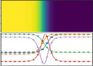
  $T_1$. The density and temperature increase rapidly across the narrow width of the shock. Owing to different relaxation times for momentum and energy transport, the temperature rises much earlier than the density, as shown in figure 1, suggesting a spatial lag between the temperature and density profiles.

Figure 1. Schematic of the internal structure of a one-dimensional normal shock wave. Temperature and density profiles are normalized as  $T_n = (T - T_0)/(T_1 - T_0)$ and $\rho _n = (\rho - \rho _0)/(\rho _1 - \rho _0)$.
The stationary field equations for mass, momentum and energy conservation, equations (2.1)–(2.3), can be obtained as
 $$\begin{gather} \frac{{\textrm{d}}}{\textrm{d}\kern0.7pt x} \left[\rho (x) u (x) \right] = 0, \end{gather}$$
 $$\begin{gather}\rho (x) u (x) \frac {{\textrm{d}}u (x) }{\textrm{d}\kern0.7pt x} ={-} \frac{{\textrm{d}}p (x)}{\textrm{d}\kern0.7pt x} - \frac{{\textrm{d}} \sigma }{\textrm{d}\kern0.7pt x}, \end{gather}$$
 $$\begin{gather}u(x) \frac {{\textrm{d}} \rho(x) \epsilon(x)}{\textrm{d}\kern0.7pt x} ={-} \frac{{\textrm{d}}q}{\textrm{d}\kern0.7pt x} - p(x)\frac{{\textrm{d}}u(x)}{\textrm{d}\kern0.7pt x} - \sigma \frac{{\textrm{d}}u(x)}{\textrm{d}\kern0.7pt x}, \end{gather}$$
where the normal stress  $\sigma _{xx}$ and the $x$-component of the heat flux vector are represented by $\sigma$ and $q$, respectively. For a dilute, monatomic gas system, we have the ideal gas equation and the internal energy of a monatomic gas without internal degrees of freedom as
 \begin{equation} p = \rho R T,\quad \epsilon = \tfrac{3}{2} R T. \end{equation}
Substituting for  $p$ and $\epsilon$, we obtain
 $$\begin{gather} \frac{{\textrm{d}}}{\textrm{d}\kern0.7pt x} \left[\rho u \right] = 0, \end{gather}$$
 $$\begin{gather}\frac {{\textrm{d}}}{\textrm{d}\kern0.7pt x} [\rho u^{2} + \rho R T + \sigma ] = 0, \end{gather}$$
 $$\begin{gather}\frac {{\textrm{d}}}{\textrm{d}\kern0.7pt x} [\rho u^{3} + 5 \rho R T u + 2 u \sigma + 2 q] = 0. \end{gather}$$
The above equations can be readily integrated between the upstream and downstream equilibrium states to obtain the well-known Rankine–Hugoniot conditions as
 $$\begin{gather} \rho_0 u_0 = \rho_1 u_1 \end{gather}$$
 $$\begin{gather}\rho_0 u_0^{2} + \rho_0 R T_0 = \rho_1 u_1^{2} + \rho_1 R T_1 \end{gather}$$
 $$\begin{gather}u_0^{2} + 5 R T_0 = u_1^{2} + 5 R T_1 . \end{gather}$$
Note that, in both of the equilibrium states, there are no gradients of velocity or temperature, thereby giving  $\sigma =0$ and $q=0$. When integration is performed between the upstream state and any point inside the shock, we obtain
 $$\begin{gather} \rho_0 u_0 = \rho u, \end{gather}$$
 $$\begin{gather}\rho_0 u_0^{2} + \rho_0 R T_0 = \rho u^{2} + \rho R T + \sigma, \end{gather}$$
 $$\begin{gather}\rho_0 u_0^{3} + 5 \rho_0 R T_0 u_0 = \rho u^{3} + 5 \rho R T u + 2 u \sigma + 2 q . \end{gather}$$
The non-dimensionalization of the  $x$-momentum and energy equations is carried out following Torrilhon & Struchtrup (Reference Torrilhon and Struchtrup2004) as
 \begin{equation} \tilde{\rho} = \frac{\rho}{\rho_{0}}, \quad \tilde{u} = \frac{u}{\sqrt{R T_0}}, \quad \tilde{T} = \frac{T}{T_{0}}, \quad \tilde{\sigma} = \frac{\sigma}{\rho_{0} R T_0}, \quad \tilde{q} = \frac{q}{\rho_{0} \sqrt{R T_0}^{3}}, \end{equation}
and the space coordinate is non-dimensionalized as
 \begin{equation} \tilde{x} = \frac{x \rho_{0} \sqrt{R T_0}}{\mu_0} ,\end{equation}
where  $\mu _0$ is the viscosity at the upstream state. The general trend in the literature is to show the variation of the hydrodynamic fields across the shock against the Alsmeyer space coordinate, $x/\lambda _0$, and we follow the same in the present study. Accordingly, the mean free path at the upstream state can be calculated as (Alsmeyer Reference Alsmeyer1976; Torrilhon & Struchtrup Reference Torrilhon and Struchtrup2004),
 \begin{equation} \lambda_0 = \frac{4}{5} \frac{\mu_0}{\rho_0 \sqrt{\frac{{\rm \pi} R T_0}{8}}}, \end{equation}
and the relation between Alsmeyer's space coordinate,  $x/\lambda _0$ and the dimensionless space variable $\tilde {x}$ becomes
 \begin{equation} \frac{x}{\lambda_0} = \frac{5}{4} \sqrt{\frac{\rm \pi}{8}} \tilde{x} \approx 0.783 \tilde{x}. \end{equation}
The Mach number ( $Ma$) defined on the basis of upstream velocity is
 \begin{equation} Ma = \frac{u_0}{\sqrt{\gamma R T_0}} = \sqrt{\frac{3}{5}} \widetilde{u_0}, \end{equation}
where  $\gamma$ is the specific heat ratio and for a monatomic gas, $\gamma = 5/3$.
The dimensionless variables in front of the shock at the upstream equilibrium state are
 \begin{equation} \widetilde{\rho_0} = 1, \quad \widetilde{u_0} = \sqrt{\frac{5}{3}} Ma, \quad \widetilde{T_0} = 1. \end{equation}
In non-dimensionalized form, the mass (3.11),  $x$-momentum (3.12) and energy (3.13) equations using (3.19a–c) can be written as
 $$\begin{gather} \widetilde{u_0} = \tilde{\rho} \tilde{u} \end{gather}$$
 $$\begin{gather}\widetilde{u_0}^{2} + 1 = \tilde{\rho} \tilde{u}^{2} + \tilde{\rho} \tilde{T} + \tilde{\sigma} \end{gather}$$
 $$\begin{gather}\tilde{u}_0^{3} + 5 \widetilde{u_0} = \tilde{\rho} \tilde{u}^{3} + 5 \tilde{\rho} \tilde{T} \tilde{u} + 2 \tilde{u} \tilde{\sigma} + 2 \tilde{q}. \end{gather}$$
Supposing  $\xi = \sqrt {\frac {5}{3}} Ma$ and removing the tildes for better readability, the above equations become,
 $$\begin{gather} \xi = \rho u \end{gather}$$
 $$\begin{gather}\xi^{2} + 1 = \rho u^{2} + \rho T + \sigma \end{gather}$$
 $$\begin{gather}\xi^{3} + 5 \xi = \rho u^{3} + 5 \rho T u + 2 u \sigma + 2 q. \end{gather}$$
From this point onward, the analysis differs when we substitute the constitutive relationships for the stress tensor and the heat flux vector based on the Navier–Stokes and the OBurnett equations.
3.1. Reduced form of the Navier–Stokes equations
In the Navier–Stokes framework, we have linear constitutive relationships for the stress tensor and the heat flux vector which are of Knudsen order. For the shock wave flow problem, these equations reduce to
 \begin{equation} \sigma ={-} \frac{4}{3} \mu \frac{{\textrm{d}}u}{\textrm{d}\kern0.7pt x}, \quad q ={-} k \frac{{\textrm{d}}T}{\textrm{d}\kern0.7pt x}. \end{equation}
Using (3.14a–e) and (3.15), the non-dimensionalized form of these equations can be obtained as (tildes are removed)
 \begin{equation} \sigma ={-} \frac{4}{3} T^{\varphi} \frac{{\textrm{d}}u}{\textrm{d}\kern0.7pt x}, \quad q ={-} T^{\varphi} \frac{1}{Pr} \frac{\gamma}{\gamma - 1} \frac{{\textrm{d}}T}{\textrm{d}\kern0.7pt x}, \end{equation}
where the symbol  $\varphi$ denotes the viscosity exponent in the expression,
 \begin{equation} \frac{\mu}{\mu_0} = \left( \frac{T}{T_0} \right)^{\varphi} = \tilde{T}^{\varphi}. \end{equation}
The thermal conductivity  $k$ appearing in Fourier's law is replaced using expression
 \begin{equation} k = \frac{\mu R}{Pr} \frac{\gamma}{\gamma - 1}, \end{equation}
where  $Pr$ is the Prandtl number, which is $2/3$ for monatomic gases. Substituting these expressions in (3.24) and (3.25), we obtain an explicit dynamical system of two ordinary differential equations of order one as
 $$\begin{gather} \frac{{\textrm{d}}u}{\textrm{d}\kern0.7pt x} = \frac{3}{4} \frac{1}{T^{\varphi}} \left[\xi \left(u + \frac{T}{u} - \xi \right) - 1 \right], \end{gather}$$
 $$\begin{gather}\frac{{\textrm{d}}T}{\textrm{d}\kern0.7pt x} ={-} \frac{Pr}{2} \frac{\gamma - 1}{\gamma} \frac{1}{T^{\varphi}} [ \xi^{3} + 5 \xi + \xi u^{2} - 3 \xi T - 2u \xi^{2} - 2 u ]. \end{gather}$$
The space dependency can be removed by taking the derivative of the temperature with respect to velocity as,
 \begin{equation} \frac{{\textrm{d}}T}{{\textrm{d}}u} ={-} \frac{2}{3} Pr \left(\frac{\gamma - 1}{\gamma}\right) \frac{\left[ u \xi^{3} + 5 u \xi + \xi u^{2} - 3 \xi T u - 2u^{2} \xi^{2} - 2 u^{2} \right]}{\xi u^{2} + \xi T - \xi^{2} u - u}. \end{equation}
With the highest order of the differential equations being one, the orbits for the Navier–Stokes dynamical system are two-dimensional in the phase space ( $u, T$). In addition, the expression for $dT/du$ does not involve the viscosity index ( $\varphi$), implying that the orbits in the Navier–Stokes equations are independent of the viscosity index.
3.2. Reduced form of the OBurnett equations
The constitutive relationships for the normal stress and the heat flux according to the OBurnett equations can be obtained as
 \begin{equation} \sigma = \underline{\mu \delta_1 \frac{{\textrm{d}}u}{\textrm{d}\kern0.7pt x}} + 4\frac{\mu^{2} \beta }{\rho} \alpha_1\left(\frac{{\textrm{d}}u}{\textrm{d}\kern0.7pt x}\right)^{2}, \end{equation}
 \begin{align} q &= \underline{\delta_4 k \frac{1}{2 R \beta ^{2}} \frac{{\textrm{d}} \beta}{\textrm{d}\kern0.7pt x}} + 4\frac{\mu^{2} \beta }{\rho} \left[\gamma_1 \frac{1}{\beta} \frac{{\textrm{d}}g}{\textrm{d}\kern0.7pt x} \frac{{\textrm{d}}u}{\textrm{d}\kern0.7pt x} + \gamma_7 \frac{1}{\beta^{2}} \frac{{\textrm{d}} \beta}{\textrm{d}\kern0.7pt x} \frac{{\textrm{d}}u}{\textrm{d}\kern0.7pt x} \right] \nonumber\\ &\quad + \left(\frac{2k (\gamma -1)}{R \gamma} \right)^{2}\frac{1}{\rho \beta} \left[\gamma_{16} \frac{{\textrm{d}} \beta}{\textrm{d}\kern0.7pt x} \frac{{\textrm{d}}u}{\textrm{d}\kern0.7pt x} \right]. \end{align}
The underlined terms represent the Navier–Stokes contribution while the remaining terms are of the order of the Knudsen number squared and represent the OBurnett contribution. The variables  $\beta$ and $g$ appearing in the equations are given as
 \begin{equation} \beta = \frac{1}{2RT}, \quad g = \log \left(\frac{\rho}{\beta}\right) = \log \left({2 \rho R T}\right) = \log (2p), \end{equation}
and their derivatives are
 \begin{equation} \frac{{\textrm{d}} \beta}{\textrm{d}\kern0.7pt x} ={-} \frac{1}{2RT^{2}} \frac{{\textrm{d}}T}{\textrm{d}\kern0.7pt x}, \quad \frac{{\textrm{d}}g}{\textrm{d}\kern0.7pt x} = \frac{1}{p} \frac{{\textrm{d}}p}{\textrm{d}\kern0.7pt x}. \end{equation}
The coefficients appearing in (3.33) and (3.34) are given as
 \begin{equation} \left.\begin{gathered} \delta_1 ={-}\frac{4}{3};\quad \alpha_1 = \left(\frac{125\gamma^{2}- 576\gamma + \varphi(110-160\gamma + 50\gamma^{2})+643}{40}\right) =\frac{8}{15}; \\ \delta_4 = 1;\quad \gamma_1 = \left(\frac{-47+25\gamma}{8}\right) ={-} \frac{2}{3};\quad \gamma_7 = \varphi \left(\frac{77-35\gamma}{8}\right) = \frac{7}{6}; \\ \gamma_{16}=\left(\frac{-77+35 \gamma+10 \varphi ({-}1+\gamma)}{8}\right) ={-} \frac{23}{12}, \end{gathered}\right\} \end{equation}
where we have used  $\gamma = 5/3$ and $\varphi = 1/2$ for a monatomic gas composed of hard-sphere molecules.
In terms of regular variables  $\rho$, $u$ and $T$,
$T$,
 $$\begin{gather} \sigma ={-} \frac{4}{3} \mu \frac{{\textrm{d}}u}{\textrm{d}\kern0.7pt x} + 2 \alpha_1 \frac{\mu^{2}} {\rho RT} \left(\frac{{\textrm{d}}u}{\textrm{d}\kern0.7pt x}\right)^{2}, \end{gather}$$
 $$\begin{gather}q ={-} k \frac{{\textrm{d}}T}{\textrm{d}\kern0.7pt x} + 4 \gamma_1 \left(\frac{\mu}{\rho}\right)^{2} \frac{{\textrm{d}} \rho}{\textrm{d}\kern0.7pt x} \frac{{\textrm{d}}u}{\textrm{d}\kern0.7pt x} + 4 \left(\gamma_1 - \gamma_7 - \frac{\gamma_{16}}{Pr^{2}} \right) \frac{\mu^{2}}{\rho T} \frac{{\textrm{d}}u}{\textrm{d}\kern0.7pt x} \frac{{\textrm{d}}T}{\textrm{d}\kern0.7pt x}. \end{gather}$$
Performing non-dimensionalization and replacing density with velocity using (3.23)
 $$\begin{gather} \sigma ={-} \frac{4}{3} T^{\varphi} \frac{{\textrm{d}}u}{\textrm{d}\kern0.7pt x} + \frac{2 \alpha_1}{\xi} T^{2 \varphi - 1} u \left(\frac{{\textrm{d}}u}{\textrm{d}\kern0.7pt x}\right)^{2}, \end{gather}$$
 $$\begin{gather}q ={-} T^{\varphi} \frac{1}{Pr} \frac{\gamma}{\gamma - 1} \frac{{\textrm{d}}T}{\textrm{d}\kern0.7pt x} - 4 \gamma_1 \frac{T^{2 \varphi}}{\xi} \left(\frac{{\textrm{d}}u}{\textrm{d}\kern0.7pt x}\right)^{2} + 4 \varPsi \frac{T^{2 \varphi - 1}}{\xi} u \frac{{\textrm{d}}u}{\textrm{d}\kern0.7pt x} \frac{{\textrm{d}}T}{\textrm{d}\kern0.7pt x}, \end{gather}$$
where we have combined the expression  $[\gamma _1 - \gamma _7 - \gamma _{16}/Pr^{2}]$ into a single constant $\varPsi$ ( $=119/48$). Substituting these constitutive relationships in (3.24) and (3.25), we obtain an implicit dynamical system of two ordinary differential equations of order one as
 \begin{align} &- \frac{4}{3} T^{\varphi} \frac{{\textrm{d}}u}{\textrm{d}\kern0.7pt x} + \frac{2 \alpha_1}{\xi} T^{2 \varphi - 1} u \left(\frac{{\textrm{d}}u}{\textrm{d}\kern0.7pt x}\right)^{2} = \xi^{2} + 1 - \xi u - \xi \frac{T}{u}, \end{align}
 \begin{align} & - T^{\varphi} \frac{1}{Pr} \frac{\gamma}{\gamma - 1} \frac{{\textrm{d}}T}{\textrm{d}\kern0.7pt x} - 4 \gamma_1 \frac{T^{2 \varphi}}{\xi} \left(\frac{{\textrm{d}}u}{\textrm{d}\kern0.7pt x}\right)^{2} + 4 \varPsi \frac{T^{2 \varphi - 1}}{\xi} u \frac{{\textrm{d}}u}{\textrm{d}\kern0.7pt x} \frac{{\textrm{d}}T}{\textrm{d}\kern0.7pt x} \nonumber\\ &\quad = \frac{1}{2} \left[ \xi^{3} + 5 \xi + \xi u^{2} - 3 \xi T - 2u \xi^{2} - 2 u \right]. \end{align}
It is evident that obtaining an explicit expression for  $dT/du$ is not possible and the orbital structures are different for different values of the viscosity index, unlike the Navier–Stokes equations.
In matrix form, the system of equations can be represented as
 \begin{equation} \boldsymbol{A} \boldsymbol{\cdot} \frac{{\textrm{d}} \boldsymbol{y}}{\textrm{d}\kern0.7pt x} = \boldsymbol{B} ,\end{equation}
where
 $$\begin{gather} \boldsymbol{y} = \begin{pmatrix} u \\ T \end{pmatrix},\quad \boldsymbol{A} = \begin{pmatrix} - \dfrac{4}{3} T^{\varphi} + \dfrac{2 \alpha_1}{\xi} T^{2 \varphi - 1} u \dfrac{{\textrm{d}}u}{\textrm{d}\kern0.7pt x} & 0 \\ - 4 \gamma_1 \dfrac{T^{2 \varphi}}{\xi} \dfrac{{\textrm{d}}u}{\textrm{d}\kern0.7pt x} & - T^{\varphi} \dfrac{1}{Pr} \dfrac{\gamma}{\gamma - 1} + 4 \varPsi \dfrac{T^{2 \varphi - 1}}{\xi} u \dfrac{{\textrm{d}}u}{\textrm{d}\kern0.7pt x} \end{pmatrix}, \end{gather}$$
 $$\begin{gather}\boldsymbol{B} = \begin{pmatrix} \xi^{2} + 1 - \xi u - \xi \dfrac{T}{u} \\ \dfrac{1}{2} \left[ \xi^{3} + 5 \xi + \xi u^{2} - 3 \xi T - 2u \xi^{2} - 2 u \right] \end{pmatrix} . \end{gather}$$
The determinant of a lower triangular matrix  $\boldsymbol {A}$ is
 \begin{align} \text{det } \boldsymbol{A} &= \frac{4}{3} \frac{T^{2 \varphi}}{Pr} \frac{\gamma}{\gamma - 1} - \frac{16}{3} \varPsi \frac{T^{3 \varphi - 1}}{\xi} u \frac{{\textrm{d}}u}{\textrm{d}\kern0.7pt x} - \frac{2 \alpha_1}{\xi} \frac{1}{Pr} \frac{\gamma}{\gamma - 1} T^{3 \varphi - 1} u \frac{{\textrm{d}}u}{\textrm{d}\kern0.7pt x} \nonumber\\ &\quad + 8 \alpha_1 \varPsi\left(\frac{T^{2 \varphi - 1}}{\xi} u \frac{{\textrm{d}}u}{\textrm{d}\kern0.7pt x}\right)^{2} . \end{align}
The first term in (3.47) is the same as that obtained in the Navier–Stokes equations and is always positive. As the velocity gradient term is negative (velocity transforms from supersonic to subsonic) and the coefficients of all the terms are positive, all the remaining terms are also positive and the determinant of matrix  $\boldsymbol {A}$ is always positive inside the shock in the case of the OBurnett equations. The inverse of the matrix $\boldsymbol {A}$ can then be obtained as
 \begin{equation} \boldsymbol{A}^{{-}1} = \frac{1}{\text{det } \boldsymbol{A}}\begin{pmatrix} - T^{\varphi} \dfrac{1}{Pr} \dfrac{\gamma}{\gamma - 1} + 4 \varPsi \dfrac{T^{2 \varphi - 1}}{\xi} u \dfrac{{\textrm{d}}u}{\textrm{d}\kern0.7pt x} & 0 \\ 4 \gamma_1 \dfrac{T^{2 \varphi}}{\xi} \dfrac{{\textrm{d}}u}{\textrm{d}\kern0.7pt x} & - \dfrac{4}{3} T^{\varphi} + \dfrac{2 \alpha_1}{\xi} T^{2 \varphi - 1} u \dfrac{{\textrm{d}}u}{\textrm{d}\kern0.7pt x} \end{pmatrix}. \end{equation}
Subsequently, the system (3.44) can be written in the following form:
 \begin{equation} \frac{{\textrm{d}} \boldsymbol{y}}{\textrm{d}\kern0.7pt x} = \frac{\boldsymbol{C}}{\text{det } \boldsymbol{A}},\quad \text{where } \boldsymbol{C} = \boldsymbol{A}^{{-}1}\boldsymbol{B}. \end{equation}
Since the determinant does not change sign inside the shock, the issue of subshocks does not arise and the OBurnett equations give smooth shock structures at all Mach numbers, similar to the Navier–Stokes equations.
4. Numerical procedure
The inherent coupled and nonlinear form of the Navier–Stokes (3.30) and (3.31) and the OBurnett (3.42) and (3.43) equations makes it improbable to solve these equations analytically. Hence, one must make recourse to numerical methods to obtain the shock wave profiles. To solve the differential equations for the velocity and temperature, appropriate boundary conditions must be supplied, which are given by Rankine–Hugoniot conditions as
 $$\begin{gather} \text{At upstream point:} \quad {u_0}_{{\mid} x \rightarrow - \infty} = \sqrt{\tfrac{5}{3}} M_0; \quad {T_0}_{{\mid} x \rightarrow - \infty} = 1 \end{gather}$$
 $$\begin{gather}\text{At downstream point:} \quad {u_1}_{{\mid} x \rightarrow \infty} = \sqrt{\frac{5}{3}} \frac{M_0^{2} + 3}{4 M_0}; \quad {T_1}_{{\mid} x \rightarrow \infty} = \frac{ (5 M_0^{2} - 1) (M_0^{2} + 3) }{ 16 M_0^{2}}. \end{gather}$$
 In the present study, we tackle the shock wave flow problem as an initial value problem as done in the literature (Gilbarg & Paolucci Reference Gilbarg and Paolucci1953; Holian et al. Reference Holian, Patterson, Mareschal and Salomons1993; Uribe et al. Reference Uribe, Velasco and García-Colín1998, Reference Uribe, Velasco, Garcia-Colin and Diaz-Herrera2000). The system of (3.43) with conditions (4.1a,b) and (4.2a,b) is numerically solved using a variable-step, variable-order Matlab solver ode15i with a maximum order of 5. The downstream equilibrium state is disturbed by introducing perturbations and the integration is performed from the downstream point to the upstream point. The relative and absolute errors are set as  $10^{-13}$ and $10^{-14}$, respectively, in the numerical integration. The numerical results of the Navier–Stokes and the OBurnett equations are validated against the DSMC results. A brief introduction to the DSMC technique along with the set-up for the current problem is presented in the following paragraphs.
The DSMC method, devised by Bird in 1960 (Bird Reference Bird1994, Reference Bird2013), is a probabilistic molecular method based on the kinetic theory for simulation of the dilute gases. With experimental data available only for limited macroscopic quantities in rarefied gas flows, the results of the DSMC simulation technique serves as the benchmark for verifying the theoretical results. The DSMC technique is a mesoscopic technique in the sense that each simulated molecule represents a number of real molecules. The ratio of real to simulated molecules and the cells that the entire computational domain is divided into, are the important simulation parameters. The basic assumption in DSMC is that, over a small time step, molecular movement and collisions can be decoupled. The time step must be less than the mean collision time. The basic four steps in DSMC are movement, indexing, collision and sampling. The flow domain is divided into cells and cells are further subdivided into subcells. The length of the cell should be less than the local mean free path to achieve physically realistic collisions. The simulated molecules are distributed into the cells and their positions and velocities are stored and updated at all times. In the movement step, all simulated molecules are moved using the selected time step and molecular velocities. The interaction with the boundaries is simulated in this step using different models. The molecules are indexed into the cell and rearranged in an array to facilitate collisions in the indexing step. In the collision step, collision partners are selected from the same cell using the probabilistic approach. The post-collision velocities of colliding molecules are calculated using different models. Finally, the macroscopic properties are sampled from the microscopic properties in the sampling step. A large number of samples are needed to minimize the statistical scatter.
In the present study, Bird's DSMC code (Bird Reference Bird1994) for shock wave flow problems which is available on Bird's website is implemented to generate the DSMC data. The length of the computational domain is taken as 0.04 m while helium gas is selected as the working fluid. The diameter ( $d$) and molecular mass ( $m$) of helium gas are taken as (Bird Reference Bird2013)
 \begin{equation} d = 2.19 \times 10^{{-}10}\,\text{m};\quad m = 6.65 \times 10^{{-}27}\,\text{kg}. \end{equation}
The no time counter method is used to select the collision pairs. The variable soft-sphere (VSS) model is selected and for hard-sphere molecules, the parameters in the VSS model are taken as  $\varphi = 0.5$ and $\alpha = 1$. The number of simulated molecules in each cell is kept as 100 and time step is selected as $5 \times 10^{-8}\,\text {s}$. The upstream number density and temperature are specified as $2.89 \times 10^{21}\,\text {m}^{-3}$ and 160 K, respectively.
5. Results
In this section, we compare the results of the OBurnett equations for hard-sphere molecules ( $\varphi = 0.5$) with the DSMC simulation results for a wide range of Mach number. The DSMC technique furnishes a detailed and accurate structure of shock wave profiles: from the measurement of the particle distribution function inside the shock (Holtz & Muntz Reference Holtz and Muntz1983; Pham-Van-Diep, Erwin & Muntz Reference Pham-Van-Diep, Erwin and Muntz1989; Erwin, Pham-Van-Diep & Muntz Reference Erwin, Pham-Van-Diep and Muntz1991) to the variation of hydrodynamic fields across the shock. In the numerical solution of the equations, the origin of the $x/\lambda _0$ axis is selected in such a way that the velocity at $x/\lambda _0 = 0$ gives the average of the upstream and downstream values of velocities. The profiles of the Navier–Stokes, conventional Burnett and OBurnett equations come together when they are translated along $x/\lambda _0$ (Holian et al. Reference Holian, Patterson, Mareschal and Salomons1993; Uribe et al. Reference Uribe, Velasco, Garcia-Colin and Diaz-Herrera2000).
5.1. Entropic consistency of the equations
The entropic consistency of the equations is an important aspect of higher-order continuum theories. It is well known that the Navier–Stokes equations are thermodynamically consistent, i.e. they always give positive entropy generation  $\dot {\sigma }$ and thereby, obey the second law of thermodynamics. However, the same cannot be said for higher-order continuum transport equations given the complicated structure of the equations.
According to the second law of thermodynamics, the term  $\dot {\sigma }$ must be a non-negative quantity and given as
 \begin{equation} \dot{\sigma} ={-} \frac{1}{T} \sigma_{ij} \frac{\partial u_i}{\partial x_j} - \frac{1}{T^{2}} q_i \frac{\partial T}{\partial x_i} \geq 0. \end{equation}
Substituting the OBurnett closure relations for normal stress (3.38) and heat flux (3.39) in the above equation, the entropy generation inside the shock for the OBurnett equations can be obtained in dimensional form as
 \begin{align} \dot{\sigma} &= \underline{\frac{4}{3} \frac{\mu}{T} \left(\frac{{\textrm{d}}u }{\textrm{d}\kern0.7pt x}\right)^{2}} - \frac{2}{T} \alpha_1 \frac{\mu^{2}}{p} \left(\frac{{\textrm{d}}u }{\textrm{d}\kern0.7pt x}\right)^{3} + \underline{\frac{k}{T^{2}} \left(\frac{{\textrm{d}}T }{\textrm{d}\kern0.7pt x}\right)^{2}} \nonumber\\ &\quad - {4 \gamma_1} \left(\frac{\mu}{\rho T}\right)^{2} \frac{{\textrm{d}} \rho }{\textrm{d}\kern0.7pt x} \frac{{\textrm{d}}u }{\textrm{d}\kern0.7pt x} \frac{{\textrm{d}}T }{\textrm{d}\kern0.7pt x} - 4 \varPsi \frac{\mu^{2}}{\rho T^{3}} \frac{{\textrm{d}}u }{\textrm{d}\kern0.7pt x} \left(\frac{{\textrm{d}}T }{\textrm{d}\kern0.7pt x}\right)^{2}. \end{align}
 The underlined terms represent the Navier–Stokes contribution to the entropy generation and are always positive. Now, across the shock, density and temperature progressively increase from an upstream to a downstream point while velocity changes from supersonic to subsonic. As a result, the contribution to the entropy generation from the remaining higher-order terms is always positive and the overall entropy generation according to the OBurnett equations turns out to be always positive. This is illustrated through figure 2, which shows the variation of dimensionless entropy generation throughout the shock for three Mach numbers ( $Ma = 2.69, 5, 7$).

Figure 2. Entropy generation across the shock for three different Mach numbers; solid line: OBurnett; dotted line: Navier–Stokes; dashed line: conventional Burnett: (a)  $Ma = 2.69$; (b) $Ma = 5$; and (c) $Ma = 7$.
At  $Ma = 2.69$ (figure 2a), all the equations predict positive entropy generation throughout the shock. Note that this particular value is the critical Mach number above which a heteroclinic trajectory does not exist for the conventional Burnett equations (Uribe et al. Reference Uribe, Velasco, Garcia-Colin and Diaz-Herrera2000). As we go above this critical Mach number (figures 2(b) and 2(c)), the conventional Burnett equations start predicting negative entropy generation in the upstream region of the shock, thereby losing their validity. This important observation also shows that the two critical aspects: existence of a heteroclinic trajectory and thermodynamic consistency of the equations are intricately connected to each other. With respect to the OBurnett equations, it is evident that the equations obey the second law of thermodynamics by giving positive entropy generation throughout the shock for all Mach numbers, similar to the Navier–Stokes equations. In addition, a heteroclinic trajectory exists for all Mach numbers, as we show in § 5.2. This important result of positive entropy generation throughout the shock establishes the thermodynamic consistency of the OBurnett equations.
5.2. Orbital structures in phase space
After establishing the thermodynamic consistency of the equations, we next explore the orbits in the phase space ( $u - T$ plane) as obtained by the OBurnett and Navier–Stokes equations and compare with those of the DSMC results. These orbital structures in phase space give detailed information about the velocity and temperature profiles. A clear advantage in exploring these orbits is that these structures do not depend on the choice of origin, hence making it possible to compare with different choices available in the literature without any ambiguity. For example, while showing the variation of hydrodynamic fields across the shock (Alsmeyer Reference Alsmeyer1976; Salomons & Mareschal Reference Salomons and Mareschal1992; Torrilhon & Struchtrup Reference Torrilhon and Struchtrup2004; Greenshields & Reese Reference Greenshields and Reese2007), the origin is selected such that density at the origin gives the average of upstream and downstream values, whereas in some works (Holian et al. Reference Holian, Patterson, Mareschal and Salomons1993; Uribe et al. Reference Uribe, Velasco and García-Colín1998, Reference Uribe, Velasco, Garcia-Colin and Diaz-Herrera2000), the origin is selected based on the velocity parameter. As such, translating the shock profiles of other variables accordingly based on these two selection criteria will yield a different comparison with the DSMC results. However, working in a phase space removes the dependence on the space coordinate and a fair comparison with the benchmark results is possible. Further, since the results for density, heat flux and normal stress are derived from velocity and temperature profiles in the Burnett and moment frameworks, the phase plots are sufficient to describe the internal structure of shocks for all the variables.
A careful analysis of the orbital structures around the upstream point region reveals the existence of a heteroclinic trajectory. This important point regarding the existence of a heteroclinic trajectory has not drawn much attention from researchers and is somewhat trivialized in the literature. However, it is to be noted that this aspect is connected to the hydrodynamic stability of the equations beyond the Navier–Stokes regime (Garcia-Colin et al. Reference Garcia-Colin, Velasco and Uribe2008). Following the analysis given in Gilbarg & Paolucci (Reference Gilbarg and Paolucci1953), it can be shown mathematically that the heteroclinic trajectory exists for the OBurnett equations. This aspect is probed further for two different Mach numbers ( $Ma = 3, 7$) and the results clearly lend support to the existence of a heteroclinic trajectory for all Mach numbers.
The orbital structures in the phase space  $(u, T)$ for $Ma=3$ are shown in figure 3 for the Navier–Stokes and OBurnett equations. These phase plots show that the OBurnett results are in better agreement with the DSMC results as compared with the Navier–Stokes equations. The zoomed-in view in the region nearby the upstream point is shown in figure 4 where the results of the conventional Burnett equations are also included. In the case of the conventional Burnett equations, the derivatives of velocity and temperature become quite large near the upstream point. As a result, we observe oscillations near the upstream point and the phase trajectory never reaches the upstream point. As also discussed in Uribe et al. (Reference Uribe, Velasco and García-Colín1998, Reference Uribe, Velasco, Garcia-Colin and Diaz-Herrera2000), in the long time limit, a limit cycle exists for $Ma < 2.69$ whereas for higher Mach numbers, the oscillations grow rapidly and such a limit cycle eventually disappears, indicating the non-existence of the heteroclinic trajectory. However, a clear heteroclinic trajectory exists for the Navier–Stokes and OBurnett equations. The phase plots at $Ma = 7$ (figure 5) further confirm the existence of the heteroclinic trajectory for the OBurnett equations at higher Mach numbers. It is possible to extend the finding to higher Mach numbers, as discussed later in § 6.4.

Figure 3. Orbits in the (a)  $u-T$; (b) $u-u^{\prime }$; (c) $T-T^{\prime }$; and (d) $u^{\prime } - T^{\prime }$ planes for $Ma=3$.

Figure 4. Zoomed in view of the orbits in the (a)  $u-T$; (b) $u^{\prime } - T^{\prime }$ planes for $Ma=3$ near the upstream point.

Figure 5. Orbits in the (a)  $u-T$; (b) $u-u^{\prime }$; (c) $T-T^{\prime }$; and (d) $u^{\prime } - T^{\prime }$ planes for $Ma=7$.
5.3. Hydrodynamic fields across the shock
The variation of the hydrodynamic fields ( $\rho$, $u$,
$u$,  $T$,
$T$,  $\sigma$ and $q$) inside the shock for three Mach numbers, $Ma = 3, 5, 9$ is shown in figures 6, 7 and 8. The limitations of the Navier–Stokes equations come to the fore in describing the shock structures, particularly at higher Mach numbers. The shock profiles for the velocity and temperature as predicted by the Navier–Stokes equations appear to be quite narrow while the OBurnett equations predict broader profiles for these quantities, which are in good agreement with the DSMC results. For density and velocity shock profiles, the more rarefied upstream region of the shock is resolved accurately by the OBurnett equations whereas some deviation is observed in the downstream region. From the temperature plots, the DSMC results predict that temperature rises much earlier than the density, which is well captured by the OBurnett equations.

Figure 6. Variation of conserved variables ( $\rho$, $u$ and $T$) and non-conserved variables ( $\sigma$ and $q$) inside the shock at $Ma = 3$.

Figure 7. Variation of conserved variables ( $\rho$, $u$ and $T$) and non-conserved variables ( $\sigma$ and $q$) inside the shock at $Ma = 5$.

Figure 8. Variation of conserved variables ( $\rho$, $u$ and $T$) and non-conserved variables ( $\sigma$ and $q$) inside the shock at $Ma = 9$.
In theoretical formulation of continuum theories within the Burnett hydrodynamics it is well known that constitutive relationships are obtained for the stress tensor and the heat flux vector in terms of the primary variables ( $\rho$, $u$ and $T$) and their gradients. Hence, the comparison of the normal stress and heat flux inside the shock depicts the accuracy of these constitutive relationships. Moreover, these being higher-order moments (the stress tensor is a second-order moment, $\sigma _{ij} = m \int C_{\langle i} C_{j \rangle } f \,{\textrm {d}} \boldsymbol {C}$ whereas heat flux vector is a contracted third-order moment, $q_i = ({m}/{2}) \int C_i C^{2} f \,{\textrm {d}} \boldsymbol {C}$), it is believed that their profiles inside the shock are more difficult to capture. The variation of normal stress and heat flux across the shock clearly shows the inability of the linear constitutive laws of the Navier–Stokes equations (Newton's law of viscosity and Fourier's law) to capture the flow physics inside the shock. On the other hand, the higher-order terms ( $O (Kn^{2}$)) present in the OBurnett constitutive relations significantly improve upon the results of the Navier–Stokes equations and predict a much wider shock, in agreement with the DSMC results. The agreement is especially good in the upstream region of the shock; however, the peak for both normal stress and heat flux is not captured that well by the OBurnett equations.
5.4. Comparison with experimental measurements of density
In view of the extreme flow conditions and a very narrow flow domain (of the order of a few mean free paths), scarce experimental data of the hydrodynamic fields across the shock are available in the literature. In particular, accurate experimental measurements of the density field using the electron beam absorption technique are available for argon gas (see Alsmeyer (Reference Alsmeyer1976) and references therein). The numerical results of the OBurnett equations for argon gas can be obtained by taking the viscosity index  $\varphi = 0.816$ as suggested by Gilbarg & Paolucci (Reference Gilbarg and Paolucci1953), Chapman & Cowling (Reference Chapman and Cowling1970) and Bird (Reference Bird2013).
Figure 9 shows the comparison of normalized density profiles ( $\rho _n = (\rho - \rho _0) / (\rho _1 - \rho _0)$) across the shock as obtained by the OBurnett equations with the experimental results of Alsmeyer (Reference Alsmeyer1976) for two Mach numbers, namely $6.5$, and $9$. From the figure, it is clear that the density results of the OBurnett equations are in quantitative agreement with the experimental results in the upstream region whereas further improvement is desirable in the downstream region. As we know, the downstream region of the shock is characterized by high temperatures, we believe that the relation between viscosity and temperature ( $\mu \propto T^{\varphi }$) might be insufficient to capture the flow physics in the downstream region accurately. By increasing dissipation in the downstream region, accurate resolution of the density profiles can be achieved. Increased dissipation tends to smoothen out the shock profiles, thereby increasing the shock thickness in the downstream region. This can be achieved either by fine tuning the viscosity index, as is done in Greenshields & Reese (Reference Greenshields and Reese2007) and Uribe & Velasco (Reference Uribe and Velasco2018), or by applying Holian's conjecture (Holian Reference Holian1988; Holian et al. Reference Holian, Patterson, Mareschal and Salomons1993). We believe that the OBurnett theory in conjunction with Holian's conjecture or an enhanced viscosity index can resolve the density profiles accurately.

Figure 9. Comparison of normalized density profiles ( $\rho _n = (\rho - \rho _0) / (\rho _1 - \rho _0)$) obtained using the OBurnett equations with the experimental measurements of Alsmeyer (Reference Alsmeyer1976) for two different Mach numbers; (a) $Ma = 6.5$ and (b) $Ma = 9$.
5.5. Temperature–density separation
Temperature–density separation ( $\delta _{\rho -T}$) is an important parameter used to characterize the internal structure of the shock. It is defined as the distance measured between the midpoints of the temperature and density shock profiles. Since the relaxation times for momentum and energy transport are finite and different, there will always be a spatial lag between temperature and density profiles. Typically in a shock wave, temperature rises from the upstream value to the downstream value before the density, as observed in figures 6–8, and a good hydrodynamic model should capture this spatial lag accurately.
For six different Mach numbers, the values of  $\delta _{\rho -T}$ for the Navier–Stokes and OBurnett equations are compared with that of the DSMC results in table 1. It is observed that the Navier–Stokes equations severely under-predict these values while the OBurnett equations are able to predict the spatial lag reasonably well when compared with the DSMC results.
Table 1. Comparison of temperature–density parameter for the Navier–Stokes and OBurnett equations with the DSMC results.

6. Discussion
In this section, we review the structure of the OBurnett constitutive relations for the stress tensor and the heat flux vector and compare with other higher-order continuum theories. This allows us to identify the problematic terms appearing in other theories which can be the potential source of instability of the equations. An order of magnitude analysis is also performed which helps to identify the less dominant terms in the equations.
For an order of magnitude analysis, upstream quantities,  $u_0$ and $\rho _0$, and mean free path $\lambda _0$ are selected as the velocity, density and length scales, respectively. In the flow domain, the pressure difference scales as $\rho _0 u_0^{2}$ while the pressure scales as $\rho _0 c^{2}$ (from the ideal gas equation) with $c$ being the velocity of sound. Similarly, the temperature difference scales as $\rho _0 u_0^{2}/R$ while the absolute temperature scales as $\rho _0 c^{2}/R$. We normalize the stress terms by $\rho _0 u_0^{2}$ and the heat flux terms by $\rho _0 u_0^{3}$ and identify the following non-dimensional numbers as:
 \begin{equation} Ma = \frac{u_0}{c},\quad Re = \frac{\rho_{0} u_0 \lambda_0}{\mu_0}. \end{equation}
Using relation  $Kn = \sqrt {{{\rm \pi} \gamma }/{2}} ({Ma}/{\mbox { {Re}}})$, we obtain an order of magnitude for the Knudsen number as
 \begin{equation} Kn \sim \frac{Ma}{Re}. \end{equation}
For the OBurnett equations, an order of magnitude analysis can be performed for different terms in the constitutive relations for the normal stress and heat flux as (see (3.38) and (3.39))
 \begin{gather} \left.\begin{aligned} \sigma & ={-} \frac{4}{3} \mu \frac{{\textrm{d}}u}{\textrm{d}\kern0.7pt x} + \overbrace{2 \alpha_1 \frac{\mu^{2}} {\rho RT} \left(\frac{{\textrm{d}}u}{\textrm{d}\kern0.7pt x}\right)^{2}}^{(i)} \\ & \sim {O} \left({Kn}/{Ma}\right) \quad \sim {O} (Kn^{2}) \\ \end{aligned}\right\} \end{gather}
 \begin{gather} \left.\begin{aligned} q & ={-} k \frac{{\textrm{d}}T}{\textrm{d}\kern0.7pt x} + \overbrace{4 \gamma_1 \left(\frac{\mu}{\rho}\right)^{2} \frac{{\textrm{d}} \rho}{\textrm{d}\kern0.7pt x} \frac{{\textrm{d}}u}{\textrm{d}\kern0.7pt x}}^{(viii)} + \overbrace{4 \left(\gamma_1 - \gamma_7 - \frac{\gamma_{16}}{Pr^{2}} \right) \frac{\mu^{2}}{\rho T} \frac{{\textrm{d}}u}{\textrm{d}\kern0.7pt x} \frac{{\textrm{d}}T}{\textrm{d}\kern0.7pt x}}^{(ix)} \\ & \sim {O} \left({Kn}/{Ma}\right) \qquad \sim {O} (Kn^{2}) \qquad \qquad \quad \sim {O} (Kn^{2}) \end{aligned}\right\}. \end{gather}
It is observed that the Navier–Stokes terms are of the order of  $Kn/Ma$ whereas the higher-order terms in both the equations of stress and heat flux are of the order of the Knudsen number squared.
6.1. Comparison with conventional Burnett equations
For the conventional Burnett equations, expressions for the normal stress and heat flux as obtained in Uribe et al. (Reference Uribe, Velasco and García-Colín1998, Reference Uribe, Velasco, Garcia-Colin and Diaz-Herrera2000) for the normal shock wave flow problem are
 \begin{equation} \left.\begin{aligned} \sigma & ={-} \frac{4}{3} \mu \frac{{\textrm{d}}u}{\textrm{d}\kern0.7pt x} + \frac{2}{3} \frac{\mu^{2}}{\rho R T} \left\{ \overbrace{\left( \omega_1 - \frac{7 \omega_2 }{3} + \frac{\omega_6}{3} \right) \left(\frac{{\textrm{d}}u}{\textrm{d}\kern0.7pt x}\right)^{2}}^{(i)} + \overbrace{\left(\omega_4 - \omega_2\right) \frac{R}{\rho} \frac{{\textrm{d}} \rho}{\textrm{d}\kern0.7pt x} \frac{{\textrm{d}}T}{\textrm{d}\kern0.7pt x}}^{(ii)} + \overbrace{\omega_2 \frac{T}{\rho^{2}} \left(\frac{{\textrm{d}} \rho}{\textrm{d}\kern0.7pt x} \right)^{2}}^{(iii)} \right. \\ & \quad \sim {O} \left({Kn}/{Ma} \right) \qquad \qquad \qquad \sim {O} (Kn^{2}) \qquad \qquad \sim {O} (Ma^{2} Kn^{2}) \qquad \quad \sim {O} (Kn^{2}) \\ & \qquad \qquad \qquad \left.\overbrace{- \left(\omega_2 - \omega_3\right) \frac{{\textrm{d}}^{2} T}{{\textrm{d}\kern0.7pt x}^{2}}}^{(iv)} \ \ \overbrace{- \ \omega_2 \frac{T}{\rho} \frac{{\textrm{d}}^{2} \rho }{{\textrm{d}\kern0.7pt x}^{2}}}^{(v)} + \overbrace{\left(\omega_4 + \omega_5\right) \frac{1}{T} \left( \frac{{\textrm{d}}T}{\textrm{d}\kern0.7pt x} \right)^{2}}^{(vi)} \right\} \\ & \qquad \qquad \qquad \qquad \sim {O} (Kn^{2}) \quad \sim {O} (Kn^{2}) \qquad \sim {O} (Ma^{2} Kn^{2}) \end{aligned}\right\} \end{equation}
 \begin{equation} \left.\begin{aligned} q & ={-}k \frac{{\textrm{d}}T}{\textrm{d}\kern0.7pt x} + \overbrace{\frac{2}{3} \left(\theta_4 - \theta_2 \right) \frac{\mu^{2}}{\rho} \frac{{\textrm{d}}^{2} u}{{\textrm{d}\kern0.7pt x}^{2}}}^{(vii)} + \overbrace{\frac{2}{3} \theta_3 \left( \frac{\mu}{\rho}\right)^{2} \frac{{\textrm{d}}u}{\textrm{d}\kern0.7pt x} \frac{{\textrm{d}} \rho}{\textrm{d}\kern0.7pt x}}^{(viii)} + \overbrace{\left(\theta_1 - \frac{8}{3} \theta_2 + \frac{2}{3} \theta_3 + 2 \theta_5 \right) \frac{\mu^{2}}{\rho T} \frac{{\textrm{d}}u}{\textrm{d}\kern0.7pt x} \frac{{\textrm{d}}T}{\textrm{d}\kern0.7pt x}}^{(ix)} \\ & \sim {O} \left ({Kn}/{Ma} \right) \quad \sim {O} (Kn^{2}/Ma^{2}) \qquad \sim {O} (Kn^{2}) \qquad \qquad \qquad \qquad \sim {O} (Kn^{2}) \end{aligned}\right\}. \end{equation}
 An order of magnitude analysis for stresses in the conventional Burnett equations identifies four terms having  ${O} (Kn^{2})$ while two terms are of ${O} (Ma^{2} Kn^{2})$. Out of the three heat flux terms, two are of ${O} (Kn^{2})$ while the second-order derivative term of velocity is of ${O} (Kn^{2}/Ma^{2})$, which can be safely neglected at higher Mach numbers. The numerical values of coefficients appearing in the stress and heat flux equations for the conventional Burnett and OBurnett equations are given in table 2. Note that there is no discrepancy in sign between the conventional Burnett and OBurnett coefficients. As seen from the above equations, a much more simpler structure of the Burnett contribution to the normal stress and heat flux is obtained for the OBurnett equations when compared against the conventional Burnett equations. The problematic second-order derivatives terms (arising from the material derivative terms) that are present in the conventional Burnett equations are not encountered in the OBurnett equations. An order of magnitude analysis also suggests that some of these terms are insignificant at higher Mach numbers. These terms are probably responsible for the instability of the conventional Burnett equations to small wavelengths. They also create problems in the upstream region of the shock where they predict negative entropy generation, as shown in Comeaux et al. (Reference Comeaux, Chapman and MacCormack1995). This is what we observed in the upstream region where the derivatives of velocity and temperature became too large, resulting in amplified oscillations in the shock profiles and thereby, suggesting the non-existence of the heteroclinic trajectory (see figure 4). With no second-order derivative terms in the OBurnett closure relations, none of these issues surface and we have stable OBurnett equations which give smooth structures at all Mach numbers along with the existence of the heteroclinic trajectory and positive entropy generation across the shock.
Table 2. Numerical values of coefficients of different terms appearing in the stress and heat flux equations for the conventional Burnett and OBurnett equations.

6.2. Comparison with other higher-order transport equations
Another recent second-order continuum theory has been proposed by Paolucci & Paolucci (Reference Paolucci and Paolucci2018) where the authors used the entropy inequality principle and extended the constitutive equations to second order in strain rate and gradients of density and temperature. It is important to note that the theory does not have its roots in the kinetic theory of gases and the coefficients appearing in the equations are free parameters. When applied to the shock wave flow problem, this theory predicts smooth shock structures at all Mach numbers. The constitutive relations for normal stress and heat flux according to this theory read as
 \begin{align} \left.\begin{aligned} \sigma & ={-} \frac{4}{3} \mu \frac{{\textrm{d}}u}{\textrm{d}\kern0.7pt x} - k^{{\ast}^{\prime}} \frac{\mu^{2}}{\rho T^{2}} \left( \frac{{\textrm{d}}T}{\textrm{d}\kern0.7pt x} \right)^{2} - k^{{\ast}{\ast}^{\prime}} \frac{\mu^{2}}{\rho^{2} T} \frac{{\textrm{d}} \rho}{\textrm{d}\kern0.7pt x} \frac{{\textrm{d}}T}{\textrm{d}\kern0.7pt x} \\ & \sim {O} (Kn/Ma) \quad \sim {O} (Ma^{2} Kn^{2}) \quad \sim {O} (Ma^{2} Kn^{2}) \end{aligned}\right\} \end{align}
 \begin{align} \left.\begin{aligned} q & ={-} k \frac{{\textrm{d}}T}{\textrm{d}\kern0.7pt x} - k^{{\ast}{\ast}^{\prime}} \left(\frac{\mu}{\rho}\right)^{2} \frac{{\textrm{d}} \rho}{\textrm{d}\kern0.7pt x} \frac{{\textrm{d}}u}{\textrm{d}\kern0.7pt x} - k^{{\ast}^{\prime}} \frac{\mu^{2}}{\rho T} \frac{{\textrm{d}}u}{\textrm{d}\kern0.7pt x} \frac{{\textrm{d}}T}{\textrm{d}\kern0.7pt x} \\ & \sim {O} (Kn/Ma) \quad \sim {O} (Kn^{2}) \qquad \sim {O} (Kn^{2}) \end{aligned}\right\}. \end{align}
Comparing these relations with that of OBurnett relations (3.38) and (3.39), we find that the terms in heat flux equation are exactly similar whereas the OBurnett expression for normal stress (3.38) has only a velocity gradient square term while (6.7) has a temperature gradient square term in addition to one more term. Both the higher-order terms are found to be  ${O} (Ma^{2} Kn^{2})$, suggesting these terms to be dominant at higher Mach numbers. The parameters $k^{\ast ^{\prime }}$ and $k^{\ast \ast ^{\prime }}$ appearing in (6.7) and (6.8) are given as
 \begin{equation} k^{{\ast}^{\prime}} = k^{{\ast}} \left( \frac{\rho T}{\mu^{2}} \right),\quad k^{{\ast}{\ast}^{\prime}} = k^{{\ast}{\ast}} \left( \frac{\rho}{\mu} \right)^{2}, \end{equation}
where  $k^{\ast }$ and $k^{\ast \ast }$ are functions of density and temperature,
 \begin{equation} k^{{\ast}} = k^{{\ast}}_0 \rho^{\beta_4} T^{\gamma_4},\quad k^{{\ast}{\ast}} = k^{{\ast}{\ast}}_0 \rho^{\beta_5} T^{\gamma_5} \end{equation}
The  $\beta$ and $\gamma$ appearing in above equation are free parameters and their values are selected in order to obtain good quantitative agreement of the density profiles with the experimental measurements. Hence, the parameters $k^{\ast ^{\prime }}$ and $k^{\ast \ast ^{\prime }}$ are more or less fitting parameters and lack a derivation from first principles. This is not the case in the OBurnett equations since there are no free parameters and all the OBurnett coefficients come from kinetic theory.
Comparison with the nonlinear coupled constitutive relations (NCCR) theory proposed by Myong (Reference Myong1999) can also be done. This theory is thermodynamically consistent at every order of approximation (Myong Reference Myong1999; Tang & Xiao Reference Tang and Xiao2017) and is based on the generalized hydrodynamics equations proposed by Eu (Eu Reference Eu1980; Al-Ghoul & Eu Reference Al-Ghoul and Eu1997). The partial differential equations for the stress tensor and heat flux vector are transformed into nonlinear coupled algebraic equations using the adiabatic approximation (Myong Reference Myong1999). The corresponding relations for the shock wave flow problem are obtained as (Jiang et al. Reference Jiang, Zhao, Chen and Agarwal2019; Liu, Yang & Zhong Reference Liu, Yang and Zhong2019),
 $$\begin{gather} \sigma = \frac{1}{\tilde{q} (\kappa)} \frac{\mu}{p} \left\{ - \frac{4}{3} \frac{{\textrm{d}}u}{\textrm{d}\kern0.7pt x} \left(p + \sigma \right) \right \} \end{gather}$$
 $$\begin{gather}q = \frac{1}{\tilde{q} (\kappa)} \frac{\mu}{p} \frac{1}{Pr} \left\{ - \left( p + \sigma \right) C_p \frac{{\textrm{d}}T}{\textrm{d}\kern0.7pt x} - \frac{{\textrm{d}}u}{\textrm{d}\kern0.7pt x} q \right\} , \end{gather}$$
where  $\tilde {q} (\kappa )$ is a nonlinear dissipation factor. Note that the equations are implicit, coupled and can be solved by iterative methods like the Newton method for given values of conserved variables and their derivatives. A simple exercise of substituting for $\sigma$ and $q$ on the right-hand side of (6.11) and (6.12) using the Navier–Stokes linear constitutive laws can make the equations explicit. The relation for normal stress is then similar in structure to the OBurnett stress relation (6.3) although the coefficients are different. For the heat flux relation, we see that the NCCR relation (6.12) is a subset of the OBurnett relation (6.4) where one additional term involving the product of the gradient of density and velocity is present in the OBurnett theory (second term in (6.4)).
Some recent works have obtained shock profiles within the Navier–Stokes framework and important remarks can be made in this context. In the work of Uribe & Velasco (Reference Uribe and Velasco2018), the viscosity index was enhanced (greater than one) and fine tuned so as to obtain quantitative agreement of density profiles with the experimental results; however, temperature profiles were markedly different when compared with the DSMC results. An attempt for the enhancement in viscosity can be traced to Holian's work (Holian Reference Holian1988; Holian et al. Reference Holian, Patterson, Mareschal and Salomons1993). The conjecture proposed by Holian was to use the temperature component in the direction of the shock wave propagation,  $T_{xx}$, in computing the linear transport coefficients instead of the mean temperature ( $T = (T_{xx} + T_{yy} + T_{zz})/3$). Since $T_{xx}$ is almost twice that of $T$, significant enhancement in viscosity is achieved, which results in better agreement between the Navier–Stokes and molecular dynamics results (He, Tang & Pu Reference He, Tang and Pu2008; Velasco & Uribe Reference Velasco and Uribe2021).
6.3. Comparison with moment equations
We now make some important remarks in the context of the moment equations and their results for the shock wave problem. In the moment framework, we encounter complex production terms coming from the collision integral in the transport equations for the stress tensor and the heat flux vector. These production terms signify the net gain of stresses or heat flux due to intermolecular collisions. For Maxwell molecules, these production terms can be evaluated in closed form without knowledge of the distribution function (Truesdell & Muncaster Reference Truesdell and Muncaster1980). However, for other interaction potentials, evaluation of these integrals is extremely cumbersome and their exact form is not known, although a linearized form of the R13 equations based on an order of magnitude method has been derived for an arbitrary interaction potential (Struchtrup & Torrilhon Reference Struchtrup and Torrilhon2012, Reference Struchtrup and Torrilhon2013). Recently, Cai & Wang (Reference Cai and Wang2020) proposed R13 moment equations for hard-sphere molecules where these production terms are evaluated by considering the linearized form of the collision integral. These equations are extremely complex and have a drastically different form when compared with the Grad 13 moment equations. This also suggest different sets of governing equations for different interaction potentials in the moment framework, which is not the case in Burnett hydrodynamics. In Burnett theories, the effect of the interaction potential is expressed through the Burnett coefficients and the viscosity index.
The effect of the interaction potential is embodied in the collision integral of the Boltzmann equation. In the derivation of the Grad distribution function, there is no active involvement of the Boltzmann equation (and thereby collision integral) and hence the interaction potential does not appear explicitly in the Grad distribution function. On the other hand, in Burnett theories, the perturbed series of the distribution function is substituted in the Boltzmann equation to obtain successive approximations of the distribution function. As such, the distribution function employed in Burnett theories is general for all interaction potentials.
The application of the R13 moment equations to shock wave flow problems for Maxwell molecules described shock profiles accurately when compared with the DSMC results (Torrilhon & Struchtrup Reference Torrilhon and Struchtrup2004). However, an extension of the R13 equations to hard-sphere molecules by changing the viscosity index did not yield satisfactory results. The authors remarked that the validity of the R13 moment equations is questionable for  $Ma > 4$; however, recent works by Timokhin et al. (Reference Timokhin, Bondar, Kokhanchik, Ivanov, Ivanov and Kryukov2015, Reference Timokhin, Struchtrup, Kokhanchik and Bondar2016, Reference Timokhin, Struchtrup, Kokhanchik and Bondar2017) show that the applicability of the R13 equations can be extended up to a Mach number equal to 8 for different interaction potentials. When shock profiles are evaluated by the R13 equations for hard-sphere molecules proposed by Cai & Wang (Reference Cai and Wang2020), the results agreed well with the DSMC results. However, the high complexity in the collision terms puts a serious limitation on the usage of these equations.
6.4. Advantages of using the OBurnett equations
With above critical comments, we now make some important remarks with respect to the OBurnett equations. In our earlier work (Jadhav & Agrawal Reference Jadhav and Agrawal2020b), the case of a very strong shock ( $Ma = 134$) was studied using the OBurnett equations wherein several fundamental aspects of the equations were established. Without tweaking the equations in any way, mathematical evidence was put forward for the following important aspects:
(i) Smooth shock structures at all Mach numbers.
(ii) Existence of a heteroclinic trajectory at all Mach numbers.
(iii) Positive entropy generation across the shock at all Mach numbers.
It is important to note that the conventional Burnett equations and the Grad 13 moment equations do not satisfy all these fundamental aspects. For example, the conventional Burnett equations are unstable, thermodynamically inconsistent and a heteroclinic trajectory does not exist for the shock wave flow problem. On the other hand, the Grad 13 moment equations suffer from subshocks. In addition, the Burnett and moment equations require additional boundary conditions for the complete solution, which are difficult to prescribe. Since there are no higher-order derivatives in the OBurnett equations, well-established velocity slip and temperature jump boundary conditions are sufficient for the complete solution. All these aspects clearly show that the OBurnett equations have significant advantages when compared with the conventional Burnett or the Grad moment equations and can be applied to complex flow problems without any restrictions.
The significant results achieved with the OBurnett equations can be attributed to the Onsager-consistent approach (Singh & Agrawal Reference Singh and Agrawal2016; Singh et al. Reference Singh, Jadhav and Agrawal2017) followed in the derivation of the equations. The distribution function formulated at the microscopic level is consistent with Onsager's symmetry principle. When projected onto the macroscopic level by deriving the closure relations for the stress tensor and the heat flux vector, we obtain OBurnett equations that comply with the principles of non-equilibrium thermodynamics. There is no ad hoc addition or deletion of terms as we see in some of the variants of higher-order continuum theories. Further, in obtaining shock profiles, the equations are neither tweaked in any way nor there are any free parameters. Hence, with a sound physical basis, it is not surprising that the OBurnett equations are entropically consistent, give smooth shock structures at all Mach numbers and, at the same time, significantly improve upon the results of the Navier–Stokes equations. With sound physical results for the shock waves, the next important step is to apply the OBurnett equations for other important non-equilibrium flows in rarefied gas dynamics which will help to firmly establish the validity of the equations. This exercise is currently in progress and we aim to report it in our future works.
7. Conclusions
In the present study, the internal structure of a one-dimensional normal shock wave is studied using the recently derived OBurnett equations. In our previous work (Jadhav & Agrawal Reference Jadhav and Agrawal2020b), the equations were shown to give smooth shock structures at all Mach numbers with positive entropy generation across the shock and the clear existence of a heteroclinic trajectory for a demanding case of a strong shock ( $Ma =134$). In the present work, the aim was to verify these claims for a wide range of Mach numbers ( $3 \leq Ma \leq 9$) with a special emphasis on the orbital structures in the phase space.
The problem was solved as an initial value problem for a dilute gas system composed of hard-sphere molecules and the numerical results of the OBurnett equations were benchmarked against the in-house DSMC results. The orbital structures of the OBurnett equations in the phase space clearly suggested the existence of a heteroclinic trajectory for all Mach numbers; a significant result in the sense that such a trajectory does not exist for the conventional Burnett equations for  $Ma > 2.69$. The thermodynamic consistency of the OBurnett equations was also established by showing positive entropy generation throughout the shock for all Mach numbers. The intricate connection between the existence of the heteroclinic trajectory and the thermodynamic consistency of the equations was highlighted, where we observed that thermodynamic consistency of the equations guarantees the existence of the heteroclinic trajectory. The OBurnett constitutive relations for the stress tensor and heat flux vector are reviewed and compared against that of the conventional Burnett equations and other higher-order continuum theories and important remarks are made in the context of stability of the equations. The results of the OBurnett equations for the variation of hydrodynamic fields across the shock also showed substantial improvement over those of the Navier–Stokes equations. The agreement between the OBurnett and the DSMC results is quantitative, especially in the upstream region of the shock. These significant results firmly establish the Onsager-consistent approach in the underlying derivation of the OBurnett equations.
We believe that with a strong fundamental basis and no arbitrary assumptions, the OBurnett equations are not restricted to small Knudsen number flows and are expected to discern flow physics in strong non-equilibrium flows better than the Navier–Stokes equations, which we have shown here for shock waves. With Chapman–Enskog based Burnett equations and the Grad moment equations valid for a small Mach number range, the present work assumes significance and puts forward an improved theory for shock waves with no upper Mach number limit.
Acknowledgements
This work was done as part of the Department of Atomic Energy Science Research Council Outstanding Investigator Award (21/01/2015-BRNS/35038).
Declaration of interests
The authors report no conflict of interest.


 Open access