


1 Introduction
Transferring the value of a statistical life (VSL) from one nation to another is critical in valuing mortality risk reduction benefits in benefit-cost analyses for countries that lack reliable domestic VSL estimates. Benefit transfer is particularly important for lower income countries, which often lack stated preference evidence of the VSL and which rarely have sufficient reliable occupational fatality and employment data to estimate the VSL using revealed preference data, as in labor market studies of the VSL. Transferring VSL estimates from one country to another requires a baseline VSL and its associated income level, the income level for the country of interest, and the income elasticity of the VSL. The dependence of the VSL on income has a well-established theoretical basis and is amenable to empirical analysis given the availability of international income data. Of course, life expectancy, age, health, religion, and culture also will likely affect individual valuation of mortality risks, but researchers do not currently have a robust understanding of how non-income factors affect the VSL (Robinson et al., Reference Robinson, Hammitt and O’Keeffe2018). As a result, researchers have devoted significant attention to estimating the income elasticity of the VSL, which is the critical parameter in benefit transfer calculations. Despite substantial efforts, the literature has not reached a consensus about what income elasticity of the VSL should be used when transferring VSL estimates to countries with much lower income levels than the average in U.S. studies.
Studies using different samples and different methodologies have led to sometimes divergent values, leading researchers such as Hammitt and Robinson (Reference Hammitt and Robinson2011) and Narain and Sall (Reference Narain and Sall2016) to generally conclude that higher elasticities are appropriate in lower income economies than in wealthier economies.Footnote 2 For example, Narain and Sall (Reference Narain and Sall2016) recommend a VSL income elasticity of 1.2 for lower and middle income countries and an elasticity of 0.8 for higher income countries. However, no study has empirically specified the nature of the relationship between the VSL income elasticity and income based on stated preference evidence, which is more likely to include very low income countries in the sample. This article presents a meta-analysis of stated preference estimates of the VSL to analyze the variation in the income elasticity across countries, demonstrating that the income elasticity of the VSL is approximately 1.0 for all countries with VSLs lower than $2 million and approximately 0.55 for all countries with VSLs greater than $2 million.Footnote 3 In our specifications most appropriate for use in benefit transfer, we find that VSLs above $2 million have an income elasticity of 0.85. Because the VSL is often not known before undertaking the benefit transfer, we also present results on the variation of the VSL income elasticity with the per capita income in the country.
In Section 2, we review the literature estimating the income elasticity of the VSL. While the evidence is broadly consistent with lower income economies having higher VSL income elasticities, the estimates demonstrate significant heterogeneity in methodology and results. Nevertheless, this review is useful since we find some similarities in the income elasticities based on stated preference studies and some revealed preference evidence. Section 3 presents our meta-analysis datasets. This analysis begins using 937 VSL estimates from the meta-analysis sample of stated preference studies in Lindhjem et al. (Reference Lindhjem, Navrud, Braathen and Biausque2011) and OECD (2012). This sample includes VSL estimates from 76 different studies and 23 different countries. We also augment our base sample with 208 observations from nine stated preference studies presented in Robinson et al. (Reference Robinson, Hammitt and O’Keeffe2018), which gathered stated preference articles on the VSL in low and middle income countries. These low income country estimates expand our ability to explore the difference in elasticities between high income and low income economies. The augmented sample includes estimates from 27 different countries.
Section 4 presents meta-regression estimates of the income elasticity of the VSL. These estimates indicate that the income elasticity at the mean of the VSL distribution is between 0.65 and 0.80. However, mean regressions are only informative of the income elasticity at the mean of the VSL distribution. In Section 5, we use quantile regression estimates of the VSL income elasticity to explore how the elasticity varies over the distribution of the VSL. Our results demonstrate that the income elasticity is significantly larger for smaller VSL values, reaching values between 1.0 and 1.1 for the lowest portions of the distribution. Across our specifications, we find evidence that the elasticity declines to 0.55–0.85 by the largest portions of the distribution. Section 6 discusses our results and explores their implications for VSL benefit transfer. We extend the benefit transfer equation derived in Hammitt and Robinson (Reference Hammitt and Robinson2011) to account for the stepped income elasticity that we observe in our results. Using our recommendations to transfer VSLs to lower income economies generally results in higher VSLs than those currently adopted for policy purposes; the effect is largest for the lowest income economies.
Table 1 Literature review.

2 Income elasticities literature review
Table 1 provides a brief summary of estimates of the income elasticity of the VSL from 24 studies. Most of the studies are meta-analyses in which the VSL estimates from multiple studies are pooled in a sample for which the VSL differences across income levels are estimated. The large number of such meta-analyses has also led to one study (Doucouliagos et al., Reference Doucouliagos, Stanley and Viscusi2014) that is a meta-meta-analysis in which the income elasticity estimates from previous meta-analyses serve as the dependent variable of interest rather than the VSL. Cross-country comparisons and quantile regression estimates for a single sample also have been used. The main contrast is between results from stated preference studies and labor market revealed preference studies. Within each of these groups, there are estimates based on single samples involving money-risk tradeoffs for people at different income levels, as well as meta-analyses of estimates of this type.
Estimates of the income elasticity of the VSL using estimates from (mostly U.S.) labor market studies have consistently found elasticities close to 0.6, including studies by Viscusi and Aldy (Reference Viscusi and Aldy2003) (0.46–0.61), Bellavance et al. (Reference Bellavance, Dionne and Lebeau2009) (0.4–0.75), and Doucouliagos et al. (Reference Doucouliagos, Stanley and Viscusi2014) (0.25–0.63). Some labor market studies have found higher values, including the publication selection bias analysis by Viscusi (Reference Viscusi2015) (0.76–1.1), the long-term longitudinal analysis by Costa and Kahn (Reference Costa and Kahn2004) (1.5–1.7), and the quantile regression analysis of a single labor market sample by Kniesner et al. (Reference Kniesner, Viscusi and Ziliak2010) (1.23–2.24), but these studies have all had distinctive aspects to the research approach. A labor market study by Viscusi and Masterman (Reference Viscusi and Masterman2017b ) containing estimates from lower income countries found an income elasticity near 1.1 for the international sample and a range of 0.5–0.7 for the U.S. sample. That study is closest methodologically to this article.
However, the VSL estimates that we focus on here are based on stated preference studies rather than labor market studies. There have been some income elasticity estimates derived from estimates across a sample of individual stated preference responses, such as that in Hoffmann et al. (Reference Hoffmann, Krupnick and Qin2017), who estimated an elasticity of 0.2–0.6 in China. Another approach is that of cross-country comparisons, as in Hammitt and Ibarrarán (Reference Hammitt and Ibarrarán2006), who estimated an elasticity range of 1.4–2.0. The meta-analysis of stated preference studies by Lindhjem et al. (Reference Lindhjem, Navrud, Braathen and Biausque2011) and the OECD (2012) found an income elasticity range from 0.7 to 1.3. That study is the closest antecedent to ours in terms of the data used, but our empirical analysis more closely follows that in Viscusi and Masterman (Reference Viscusi and Masterman2017b ).
3 Data
Our base sample is drawn from the database of stated preference VSL estimates published by the OECD.Footnote 4 Lindhjem et al. (Reference Lindhjem, Navrud, Braathen and Biausque2011) and OECD (2012) used the same database to construct their samples. The OECD database contains 1013 estimates of the VSL. We drop five estimates because they were either meta-analyses themselves or were median VSL estimates. Finally, we drop 71 observations for which neither the sample size nor standard error of the VSL estimate was available. Having either the VSL standard error or the sample size is essential to being able to know the standard error or to construct an estimate of the standard error of the VSL, which will be the critical variable in our publication bias-corrected estimates of the income elasticity. Dropping these estimates leaves us with the 937 observations that form the basis for our initial analysis. Our analyses then augment this sample using studies identified in Robinson et al. (Reference Robinson, Hammitt and O’Keeffe2018), which reviewed the VSL literature for studies measuring the VSL in low and middle income countries. Of the 17 stated preference studies in their review, nine stated preference studies containing 243 estimates were not already included in our base sample. After omitting estimates according to the same criteria as for our base sample, 208 observations remained, yielding an augmented sample of 1145 stated preference VSL estimates.
Table 2 provides summary statistics for both of our samples. The mean VSL in our base sample is $10.3 million, while the mean value in the augmented sample is a lower value of $8.5 million. The mean estimate in the base sample has a standard error of $4.2 million, while the mean standard error in the augmented sample is $3.5 million.Footnote 5 The estimates are drawn from a diverse group of countries based on the World Bank’s income group classifications.Footnote 6 In the base sample, 12.6% of the estimates are from the United States, 62.1% are from other high income countries, 23.4% are from upper-middle income countries, and the remaining 1.9% are from lower-middle income countries. For the augmented sample, 10.3% of estimates are from the United States, 51.3% of estimates are from other high income countries, 31.2% of estimates are from upper-middle income countries, and the remaining 7.2% are from lower-middle income countries.
Table 2 Summary statistics.

Note: $N=937$
for the base sample and
$N=937$
for the base sample and $N=1145$
for the augmented sample. Standard deviations in parentheses.
$N=1145$
for the augmented sample. Standard deviations in parentheses.
The mean fatality risk change presented to the survey respondents in the base sample was 3.8 deaths per 1000 individuals, and the mean fatality risk change in the augmented sample was 3.5 deaths per 1000 individuals. These fatality risks are more than an order of magnitude larger than the average fatality risk of 1 death per 10,000 workers in labor market studies generally or the average fatality risk of 1 death per 25,000 workers in studies using the Census of Fatal Occupational Injuries (CFOI) as summarized in Viscusi and Masterman (Reference Viscusi and Masterman2017a ,Reference Viscusi and Masterman b ). Approximately half of the stated preference estimates in both samples used health risk scenarios to calculate VSLs, while roughly 30% focused on traffic risks, and the remaining 20% addressed environmental risks. Very few of the estimates in our sample are willingness-to-accept (WTA) estimates of the VSL – less than 4% in both samples. Most studies analyzing stated preference VSL estimates have excluded WTA estimates from their analyses, including Lindhjem et al. (Reference Lindhjem, Navrud, Braathen and Biausque2011), OECD (2012), and Robinson et al. (Reference Robinson, Hammitt and O’Keeffe2018). Rather than drop these observations, we kept them in our sample and included a binary variable in our models including covariates to control for any effect the WTA format has on the VSL. The average income in our base sample is $35,387, while the augmented sample with more estimates from lower-middle income economies has a lower average income of $31,457. The average age of the sample used to estimate the VSL was 43.9 years in the base sample and 44.6 years in the augmented sample.Footnote 7
4 Meta-regression analysis
We use ordinary least squares to estimate the income elasticity of the VSL at the mean. The estimating equation takes the following form:
 $$\begin{eqnarray}Ln(\text{VSL}_{i})=\unicode[STIX]{x1D6FD}_{0}+\unicode[STIX]{x1D6FD}_{1}\times Ln(\text{Income}_{i})+X\unicode[STIX]{x1D6FD}+\unicode[STIX]{x1D700}_{i}.\end{eqnarray}$$
The coefficient $\unicode[STIX]{x1D6FD}_{1}$
provides the income elasticity of the VSL. We utilize a log–log specification because it is the most straightforward method for estimating the income elasticity of the VSL, as the coefficient
$\unicode[STIX]{x1D6FD}_{1}$
provides the income elasticity of the VSL. We utilize a log–log specification because it is the most straightforward method for estimating the income elasticity of the VSL, as the coefficient $\unicode[STIX]{x1D6FD}_{1}$
corresponds to the income elasticity estimate. The vector
$\unicode[STIX]{x1D6FD}_{1}$
corresponds to the income elasticity estimate. The vector $X$
includes the sample characteristics discussed in Section 2, including
$X$
includes the sample characteristics discussed in Section 2, including $Ln(\text{age})$
,
$Ln(\text{age})$
, $Ln(\text{risk change})$
, indicator variables controlling for the type of risk in the study (with traffic risk as the omitted category), and an indicator variable controlling for whether the estimate was a WTA estimate.
$Ln(\text{risk change})$
, indicator variables controlling for the type of risk in the study (with traffic risk as the omitted category), and an indicator variable controlling for whether the estimate was a WTA estimate.
In some specifications, we also include the standard error of the VSL estimate to correct for publication selection bias. Publication selection bias occurs whenever researchers selectively report and journals selectively publish estimates that fall outside of a conventionally accepted range. In the case of the VSL, publication selection tends to omit negative and small VSL estimates and inflate the income elasticity as discussed in Doucouliagos et al. (Reference Doucouliagos, Stanley and Giles2012), Viscusi (Reference Viscusi2015), and Viscusi and Masterman (Reference Viscusi and Masterman2017a ,Reference Viscusi and Masterman b ). VSL estimates should be symmetrically distributed around the true value. More precise estimates – those with lower standard errors – should be closest to the true value. If less precise estimates are systematically larger or smaller than the true value, it indicates that the sample is skewed and publication selection bias is present. Including the standard error of the VSL estimate is a procedure known as the precision effect test in that it controls for the effects of publication selection bias. The properties of this correction for publication selection bias are explored in Stanley (Reference Stanley2005, Reference Stanley2008) and Stanley and Doucouliagos (Reference Stanley and Doucouliagos2012). In the present context, controlling for publication selection bias in our sample has the added benefit of accounting for biases in the selection of studies from which we draw samples. As Robinson and Hammitt (Reference Robinson and Hammitt2015) discusses, the criteria that meta-analysis researchers use to determine whether to include particular estimates of the VSL can induce biases in the meta-analysis estimates. If the studies compiled in OECD (2012) or Robinson et al. (Reference Robinson, Hammitt and O’Keeffe2018) are systematically unrepresentative of estimates of the VSL, they will skew the sample just as publication selection bias would, allowing us to correct for such biases by including the estimated standard error in our regression.
Table 3 contains our results from estimating equation (1) on both of our samples. In the base specification, the base sample yields an income elasticity estimate of 1.09, and the augmented sample has an income elasticity of 1.05. Neither estimate is significantly different from 1.0. Adding covariates to the models decreases the income elasticity. In the base sample, the model controlling for age and estimate characteristics exhibits a VSL income elasticity of 0.80; additionally controlling for standard error decreases the point estimate to 0.79. In the augmented sample, the covariate model results in an elasticity of 0.71. As in the base sample, controlling for standard error marginally decreases the point estimate to 0.69. The standard error coefficient is statistically significant in both instances, but accounting for publication selection effects does not alter the general magnitude of the income elasticity estimate. As expected, the range of elasticity estimates for the base sample is very similar to the 0.7–0.9 estimated in Lindhjem et al. (Reference Lindhjem, Navrud, Braathen and Biausque2011). The greater difference is that the elasticity estimates for the augmented sample are about 0.10 lower than in the base sample once covariates are included in the analysis.
Table 3 VSL regressions using base and augmented samples.

Note: $N=937$
for the base sample and
$N=937$
for the base sample and $N=1145$
for the augmented sample. Dependent variable is ln(VSL). Standard errors in parentheses are robust and clustered on article from which observations are drawn. ***
$N=1145$
for the augmented sample. Dependent variable is ln(VSL). Standard errors in parentheses are robust and clustered on article from which observations are drawn. *** $p<0.01$
, **
$p<0.01$
, ** $p<0.05$
, *
$p<0.05$
, * $p<0.1$
.
$p<0.1$
.
The effects of the covariates are consistent with previous research. In the augmented sample, there is weak evidence that an increase in age is associated with a larger VSL. Given the inverse U-shaped relationship between the VSL and age found in previous research (Aldy and Viscusi (Reference Aldy and Viscusi2008)), it is unsurprising that evidence of a constant age elasticity effect is weak and only present in the studies with smaller VSLs. Studies with larger risk changes had smaller VSLs. Across the two samples, our results indicate that a 1% increase in the level of risk change a subject considers induces a 0.4% smaller VSL. The large effect of risk size is consistent with Carlsson et al. (Reference Carlsson, Johansson-Stenman and Martinsson2004), which showed that the VSL decreases rapidly as the fatality risk considered increases. Table 3 presents no evidence of a statistically significant variation of the VSL with survey context – environmental risk VSLs and health risk VSLs were statistically indistinguishable from traffic risk VSLs. This context neutrality result is in contrast with Dekker et al. (Reference Dekker, Brouwer, Hofkes and Moeltner2011), which found that VSLs calculated using traffic risks were significantly larger than context-neutral VSLs. The WTA estimates were approximately 3.6 to 6.8 times larger across the four models, with the models accounting for publication selection bias having the smaller effects. The WTA VSL premium is inconsistent with results from the labor market VSL literature (Kniesner et al., Reference Kniesner, Viscusi and Ziliak2014), but consistent with the significant evidence of a general WTA premium summarized by Horowitz and McConnell (Reference Horowitz and McConnell2002) and by Tuncçel and Hammitt (Reference Tunçel and Hammitt2014). In both samples, the coefficient on standard error is highly significant, demonstrating that the distribution of stated preference VSLs, like the distribution of labor market VSL estimates, is subject to publication selection bias.
Many other VSL meta-analyses have screened out estimates drawn from studies that lack certain indicia of quality, arguing that higher quality studies are more likely to provide accurate estimates of the VSL. However, quality is not easy to define with quantitative precision, and it will often be better to control for desirable or undesirable characteristics in a meta-regression framework. As Viscusi (Reference Viscusi2018) demonstrates, using a sample of “preferred estimates” causes large and statistically significant selection bias that inflates the VSL. Nevertheless, we construct a preferred sample from our dataset to facilitate comparisons of our estimates with those in the literature. Following Lindhjem et al. (Reference Lindhjem, Navrud, Braathen and Biausque2011) and OECD (2012), our screened sample omits estimates that: (1) lack information on the level of risk change that subjects faced; (2) use samples not representative of the geographic area they are drawn from; and (3) use a sample size smaller than 100 or are drawn from a study with a whole sample size less than 200. Screening our samples using these criteria drops 518 estimates from our base sample and 578 estimates from the augmented sample.
Table 4 estimates equation (1) using our screened sample. The results of primary interest are extremely similar. The base model income elasticities drop slightly to 0.98 and 0.94 in the base and augmented samples but remain statistically indistinguishable from 1.0. The estimated elasticities in the models with covariates are likewise somewhat smaller, but are all between 0.66 and 0.72. The risk change coefficient remains significantly negative and similar in magnitude. Screening causes the coefficient on health risks to be significant in the base sample, but the effect disappears in the augmented sample. The estimated WTA premium decreased in size as well, dropping in significance in the regressions controlling for standard error. The coefficient on standard error increased in size, as expected from the additional positive selection bias on estimates that screening creates.
Table 4 Income elasticity estimates using screened samples.

Note: $N=419$
for the base sample and
$N=419$
for the base sample and $N=567$
for the augmented sample. Dependent variable is ln(VSL). Standard errors in parentheses are robust and clustered on article from which observations are drawn. Both screened samples exclude: (1) estimates missing information on the level of risk change, (2) estimates using samples not representative of the geographic area they are drawn from, and (3) estimates using a sample smaller than 100 observations or drawn from a study with a whole sample size less than 200. Dependent variable is ln(VSL). ***
$N=567$
for the augmented sample. Dependent variable is ln(VSL). Standard errors in parentheses are robust and clustered on article from which observations are drawn. Both screened samples exclude: (1) estimates missing information on the level of risk change, (2) estimates using samples not representative of the geographic area they are drawn from, and (3) estimates using a sample smaller than 100 observations or drawn from a study with a whole sample size less than 200. Dependent variable is ln(VSL). *** $p<0.01$
, **
$p<0.01$
, ** $p<0.05$
, *
$p<0.05$
, * $p<0.1$
.
$p<0.1$
.
5 Quantile regression analysis
The results in the previous section suggest that higher VSLs may have a lower income elasticity, but they only measure the elasticity at the mean of our various samples. This section analyzes the income elasticity of the VSL at various points of the distribution using quantile regression analysis. Our estimating equation takes the following form:
 $$\begin{eqnarray}Ln(\text{VSL}_{i})^{(q)}=\unicode[STIX]{x1D6FD}_{0}^{(q)}+\unicode[STIX]{x1D6FD}_{1}^{(q)}\times Ln(\text{Income}_{i})+X\unicode[STIX]{x1D6FD}^{(q)}+\unicode[STIX]{x1D700}_{i}^{(q)}.\end{eqnarray}$$
All variables are as they were in equation (1), and $q$
denotes the quantile of the estimation. The main coefficient of interest
$q$
denotes the quantile of the estimation. The main coefficient of interest $\unicode[STIX]{x1D6FD}_{1}^{(q)}$
is the income elasticity of the VSL at the
$\unicode[STIX]{x1D6FD}_{1}^{(q)}$
is the income elasticity of the VSL at the $q$
quantile of the VSL distribution. We estimate four quantile regression models for each of our two samples: a base model, a model including covariates, and base and covariate models that add the standard error of the estimate to each model.
$q$
quantile of the VSL distribution. We estimate four quantile regression models for each of our two samples: a base model, a model including covariates, and base and covariate models that add the standard error of the estimate to each model.
Table 5 presents the results of estimating equation (2) on our base sample. For reference, Panel A provides the distribution of VSL estimates in the sample. The median estimate is $3.4 million, which is significantly smaller than the mean value of $10.3 million. The sample is significantly skewed to the right. The difference between the 95th percentile and the median is $34 million, while the difference between the 5th percentile and the median is only $3.3 million.
Table 5 Base sample quantile regressions.

Note: $N=937$
. Dependent variable is ln(VSL). Bootstrapped standard errors calculated using 500 repetitions in parentheses. Panels D and E also include ln(age), ln(risk change), and indicator variables controlling for whether the estimate was calculated using an environmental or health risk, whether the risk change information is missing, and whether the estimate was a WTA estimate. ***
$N=937$
. Dependent variable is ln(VSL). Bootstrapped standard errors calculated using 500 repetitions in parentheses. Panels D and E also include ln(age), ln(risk change), and indicator variables controlling for whether the estimate was calculated using an environmental or health risk, whether the risk change information is missing, and whether the estimate was a WTA estimate. *** $p<0.01$
, **
$p<0.01$
, ** $p<0.05$
, *
$p<0.05$
, * $p<0.1$
.
$p<0.1$
.
The remaining four panels of Table 5 present our income elasticity estimates.Footnote
8
The base estimates in Panel B indicate that the income elasticity of the VSL is relatively stable across the distribution of VSL estimates, but spikes at the 95th percentile. The estimated elasticity is between 1.0 and 1.21 until the 95th percentile, where it increases to 1.50. As Panel C shows, controlling for standard error alone eliminates the spike at the 95th percentile and demonstrates that the income elasticity of the VSL is decreasing over the length of the distribution. The income elasticity is 1.16 for the smallest VSLs, and it decreases to 0.77 for the largest VSLs. The income elasticity at the 5th percentile is significantly different from the median $(p=0.062)$
and the 95th percentile
$(p=0.062)$
and the 95th percentile $(p=0.029)$
. The large impact of including publication selection bias at the higher parts of the VSL distribution, and the increasing coefficient on standard error, demonstrate that the largest stated preference VSLs are subject to significant selection bias.
$(p=0.029)$
. The large impact of including publication selection bias at the higher parts of the VSL distribution, and the increasing coefficient on standard error, demonstrate that the largest stated preference VSLs are subject to significant selection bias.
Controlling for covariates results in lower elasticities across the distribution, but preserves the decreasing pattern from Panel C. In Panel D, we estimate an income elasticity of 1.0 for the smallest VSLs that decreases to 0.63 by the median and remains almost constant until the 90th percentile. Without controlling for standard error, the elasticity displays a slight bump at the 95th percentile. Despite the bump, there is no statistically significant difference between the estimated elasticity at the 50th, 75th, 90th, and 95th percentiles $(p=0.411)$
. In Panel E, which controls for covariates as well as publication selection bias, the median elasticity is 0.61. As in Panel C, controlling for publication selection bias eliminates the spike at the 95th percentile. The estimated coefficient on standard error is four times higher at the 95th percentile than at the 5th percentile and increases monotonically over the VSL distribution. Labor market VSL estimates in Viscusi and Masterman (Reference Viscusi and Masterman2017b
) present a similar pattern. The 5th percentile estimates are significantly different from both the median elasticity
$(p=0.411)$
. In Panel E, which controls for covariates as well as publication selection bias, the median elasticity is 0.61. As in Panel C, controlling for publication selection bias eliminates the spike at the 95th percentile. The estimated coefficient on standard error is four times higher at the 95th percentile than at the 5th percentile and increases monotonically over the VSL distribution. Labor market VSL estimates in Viscusi and Masterman (Reference Viscusi and Masterman2017b
) present a similar pattern. The 5th percentile estimates are significantly different from both the median elasticity $(p<0.001)$
and the 95th percentile
$(p<0.001)$
and the 95th percentile $(p<0.001)$
, while the elasticities in the 50th, 75th, 90th, and 95th percentiles are not significantly different from each other
$(p<0.001)$
, while the elasticities in the 50th, 75th, 90th, and 95th percentiles are not significantly different from each other $(p=0.370)$
.
$(p=0.370)$
.
Table 6 presents our results from estimating equation (2) on our augmented sample. As in Table 5, Panel A summarizes the VSL distribution, while Panels B, C, D, and E provide our estimates. The median VSL is smaller in our augmented sample ($2.1 million), as expected by adding the estimates from nine low and middle income economies. As in our base sample, the distribution exhibits significant skew. The 95th percentile estimate is $27.4 million, while the 5th percentile VSL is only $132,000.
Table 6 Augmented sample quantile regressions.

Note: $N=1145$
. Dependent variable is ln(VSL). Bootstrapped standard errors calculated using 500 repetitions in parentheses. Panels C and D also include ln(age), ln(risk change), and indicator variables controlling for whether the estimate was calculated using an environmental or health risk, whether the risk change information is missing, and whether the estimate was a WTA estimate. ***
$N=1145$
. Dependent variable is ln(VSL). Bootstrapped standard errors calculated using 500 repetitions in parentheses. Panels C and D also include ln(age), ln(risk change), and indicator variables controlling for whether the estimate was calculated using an environmental or health risk, whether the risk change information is missing, and whether the estimate was a WTA estimate. *** $p<0.01$
, **
$p<0.01$
, ** $p<0.05$
, *
$p<0.05$
, * $p<0.1$
.
$p<0.1$
.
The elasticity estimates in the augmented sample largely follow the same pattern as those in our base sample. The base estimates are stable and never significantly different from 1.0 across the distribution until the 95th percentile estimate, which jumps sharply to 1.46. Controlling for publication selection bias alone yields an elasticity that begins at 1.07 and steadily decreases to 0.78. In the covariate model, the income elasticity is 1.00 at the 5th percentile and drops to 0.52 at the median. The elasticity remains close to 0.52 relatively constant until the 95th percentile, where it jumps to 0.71. The model controlling for publication selection bias remedies the sudden jump, so that the elasticity remains between 0.50 and 0.58 over the entire distribution. In Panel E, the estimates at the 50th, 75th, 90th, and 95th percentile are all statistically indistinguishable $(p=0.532)$
. Augmenting our sample with the nine additional studies from lower income countries leaves us with the same conclusion about the relationship between the VSL and its elasticity: higher VSLs are associated with lower income elasticities.
$(p=0.532)$
. Augmenting our sample with the nine additional studies from lower income countries leaves us with the same conclusion about the relationship between the VSL and its elasticity: higher VSLs are associated with lower income elasticities.
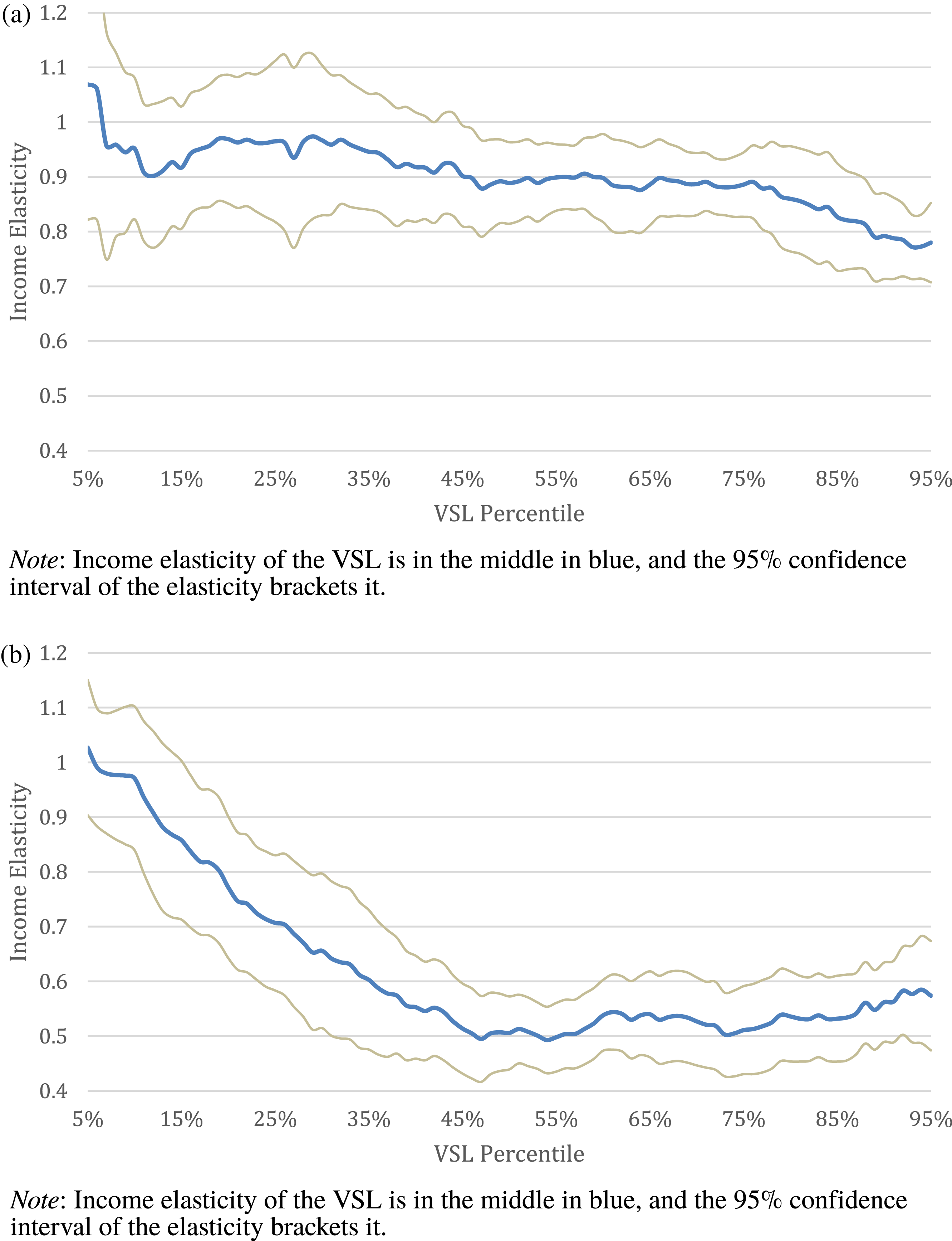
Figure 1 (a) Augmented sample income elasticity estimates (base model). (b) Augmented sample income elasticity estimates (covariate model).
Figures 1(a) and 1(b) graphically present our income elasticity estimates as a function of the VSL percentile. We create these figures by estimating the income elasticity at each of the 90 quantiles between the 5th and 95th percentiles of the distribution. Figures 1(a) and 1(b) both correspond with Table 6. Figure 1(a) presents our base income elasticity estimates, while Figure 1(b) presents our covariate models. Both figures utilize our estimates that control for publication selection bias. Consistent with our tables, in Figure 1(a) the elasticity starts around 1.1 in the base model and steadily decreases to 0.8. In the covariate model shown in Figure 1(b), the elasticity decreases smoothly over the first half of the VSL distribution before leveling off, starting close to 1.0 and settling around between 0.55 and 0.60.
While figures with percentiles on the horizontal axis are the most natural way to graphically present the results of quantile regressions, they suggest that the decrease in the income elasticity of the VSL is gradual. Because the median VSL in both samples is quite small, the decrease in the elasticity that occurs in the smaller half of the distribution is more rapid than Figures 1(a) and 1(b) suggest. To remedy this, we present Figures 2(a) and 2(b), which rescale Figures 1(a) and 1(b) by putting the VSL value rather than percentile on the horizontal axis. The figures are illuminating: in the covariate model, small VSLs have income elasticities of 1.0, but the elasticity rapidly drops to levels close to 0.55 and stays level for VSLs greater than $2 million. In the base model, the drop in the elasticity is smaller, but the vast majority of the change over the distribution has occurred once the VSLs reach $2 million. In both models, $2 million is a threshold before which the elasticity is high and rapidly declines, and after which the elasticity is nearly constant.

Figure 2 (a) Augmented sample income elasticity estimates (base model). (b) Augmented sample income elasticity estimate (covariate model).
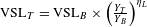
In most benefit transfer circumstances, policy makers know income levels and need a VSL to calculate the benefits of some policy. As a result, knowing the relationship between the VSL itself and the income elasticity of the VSL is of limited use. However, it is straightforward to derive a relationship between the VSL and income levels using conventional benefit transfer methods. As Hammitt and Robinson (Reference Hammitt and Robinson2011) demonstrated, assuming a constant income elasticity $\unicode[STIX]{x1D702}$
, the VSL in any country A and income (Y) and VSL in any country B have the following relationship (all else equal):
$\unicode[STIX]{x1D702}$
, the VSL in any country A and income (Y) and VSL in any country B have the following relationship (all else equal):
 $$\begin{eqnarray}\text{VSL}_{A}=\text{VSL}_{B}\times \left(\frac{Y_{A}}{Y_{B}}\right)^{\unicode[STIX]{x1D702}}.\end{eqnarray}$$
Equation (3) can be rearranged to instead calculate an income level given the VSLs of two countries as follows:
 $$\begin{eqnarray}Y_{A}=Y_{B}\times \left(\frac{\text{VSL}_{A}}{\text{VSL}_{B}}\right)^{1/\unicode[STIX]{x1D702}}.\end{eqnarray}$$
In Figures 3(a) and 3(b), we use equation (4) to estimate the relationship between the income elasticity of the VSL and income itself. For our base VSL, we adopt the U.S. VSL of $9.6 million estimated in Viscusi and Masterman (Reference Viscusi and Masterman2017a ,Reference Viscusi and Masterman b ) and Viscusi (Reference Viscusi2015). Our corresponding measure of U.S. income is the World Bank’s U.S. GNI per capita measure of $55,980. Using these base values, we iteratively estimate incomes for each quantile of the VSL distribution.Footnote 9 In our base model (Figure 3a) the income elasticity starts slightly above 1.0 at the smallest incomes, but quickly drops and remains level between 0.9 and 0.8. More dramatically, in our covariate model (Figure 3b), the income elasticity starts at about 1.0 and plummets to remain between 0.5 and 0.6. Both figures support our conclusion that the income elasticity of the VSL is close to 1.0 at very low incomes, but quickly decreases as income rises.
Table 7 Linear spline income elasticity estimates.
Note: $N=1145$
. Dependent variable is ln(VSL). Standard errors in parentheses are robust and clustered on article from which observations are drawn. The coefficients in each column are the results of three separate linear spline regression models allowing for a kink at the indicated income cutoff. Covariate models include ln(age), ln(risk change), whether the estimate was calculated using an environmental or health risk, and indicator variables controlling for whether the risk change information is missing, and whether the estimate was a WTA estimate. ***
$N=1145$
. Dependent variable is ln(VSL). Standard errors in parentheses are robust and clustered on article from which observations are drawn. The coefficients in each column are the results of three separate linear spline regression models allowing for a kink at the indicated income cutoff. Covariate models include ln(age), ln(risk change), whether the estimate was calculated using an environmental or health risk, and indicator variables controlling for whether the risk change information is missing, and whether the estimate was a WTA estimate. *** $p<0.01$
, **
$p<0.01$
, ** $p<0.05$
, *
$p<0.05$
, * $p<0.1$
.
$p<0.1$
.

Figure 3 (a) Income and income elasticity estimates (base model). (b) Income and income elasticity estimates (covariate model).
As a robustness check, in Table 7 we present estimates of the VSL income elasticity using linear spline regression.Footnote 10 Table 7 demonstrates the income elasticity of the VSL above and below three separate income thresholds: $7500, $8500, and $9500. A single threshold is the most appropriate specification as Figure 3 demonstrates the income elasticity declines until a point and then remains level. These thresholds span the income regions in which Figure 3 demonstrates a change in the VSL income elasticity. In the base and covariate versions of each model, the income elasticity is higher below the threshold, and the magnitudes are comparable to the results in our quantile regression models. We prefer our quantile regression results because they impose fewer assumptions about how the income elasticities at various parts of the distribution relate to each other; nevertheless, the spline regressions support our central finding that the income elasticity of the VSL is higher for lower income economies than higher income economies.
6 Implications for VSL transfer
Our results indicate that a straightforward application of equation (3) to transfer VSLs is inappropriate. Tables 5 and 6 and the accompanying figures demonstrate that the income elasticity is not constant for all VSLs. However, the elasticity is constant for large parts of the distribution. Equation (3) is generalizable to a situation where the income elasticity has one value above a threshold and higher value below the threshold. Let $\text{VSL}_{T}$
be the threshold VSL above which the income elasticity is
$\text{VSL}_{T}$
be the threshold VSL above which the income elasticity is $\unicode[STIX]{x1D702}_{L}$
and below which the income elasticity is
$\unicode[STIX]{x1D702}_{L}$
and below which the income elasticity is $\unicode[STIX]{x1D702}_{H}$
. Assume without loss of generality that
$\unicode[STIX]{x1D702}_{H}$
. Assume without loss of generality that $\text{VSL}_{B}>\text{VSL}_{T}$
, so that
$\text{VSL}_{B}>\text{VSL}_{T}$
, so that $\text{VSL}_{T}=\text{VSL}_{B}\times \left(\frac{Y_{T}}{Y_{B}}\right)^{\unicode[STIX]{x1D702}_{L}}$
by equation (3).Footnote
11
Then:
$\text{VSL}_{T}=\text{VSL}_{B}\times \left(\frac{Y_{T}}{Y_{B}}\right)^{\unicode[STIX]{x1D702}_{L}}$
by equation (3).Footnote
11
Then:
 $$\begin{eqnarray}\text{VSL}_{A}=\left\{\begin{array}{@{}ll@{}}\text{VSL}_{B}\times \left({\displaystyle \frac{Y_{A}}{Y_{B}}}\right)^{\unicode[STIX]{x1D702}_{L}}\quad & \text{if }Y_{A}\geqslant Y_{T},\\ \text{VSL}_{T}\times \left({\displaystyle \frac{Y_{A}}{Y_{T}}}\right)^{\unicode[STIX]{x1D702}_{H}}\quad & \text{if }Y_{A}<Y_{T}.\end{array}\right.\end{eqnarray}$$
Intuitively, equation (5) transfers the VSL from the high base VSL to the threshold VSL using the high-VSL income elasticity, and then transfers to lower VSLs using the low-VSL income elasticity and the threshold as the base VSL.Footnote 12
Our quantile regression results support using $2 million as a threshold VSL. As demonstrated in Figure 2, the income elasticity of the VSL is statistically indistinguishable from 0.85 for all VSLs greater than $2 million ( $p=0.869$
). Likewise, in our covariate model, the income elasticity of the VSL is statistically indistinguishable from 0.55 for all VSLs greater than $2 million (
$p=0.869$
). Likewise, in our covariate model, the income elasticity of the VSL is statistically indistinguishable from 0.55 for all VSLs greater than $2 million ( $p=0.964$
). In both models, most VSLs below these values have income elasticities indistinguishable from 1.0. Using equation (4) and the U.S. base VSL and income of $9.631 million and $55,980, this implies an income cutoff of $8809 in the base model and $3212 in the covariate model. The two different models imply a different income threshold because the covariate model’s lower income elasticity causes more incomes to have VSLs greater than $2 million.
$p=0.964$
). In both models, most VSLs below these values have income elasticities indistinguishable from 1.0. Using equation (4) and the U.S. base VSL and income of $9.631 million and $55,980, this implies an income cutoff of $8809 in the base model and $3212 in the covariate model. The two different models imply a different income threshold because the covariate model’s lower income elasticity causes more incomes to have VSLs greater than $2 million.
Which model is appropriate to use for benefit transfer will generally vary with the circumstances. Our base estimate income elasticity includes the effect of other factors that affect the VSL and are correlated with income. Even if we do not know how non-income factors shape the VSL within a country, using the base estimates allows us to adjust for them to the extent those factors vary with income. Because such non-income factors will usually vary across countries, using the covariate model elasticity will generally under-adjust for differences across countries. In situations where other factors are unchanged between the base and transfer estimates, such as when policy makers choose to calculate different VSLs for different purposes or groups within the same country, the smaller covariate elasticity will be appropriate. As a result, intra-country benefit transfer across time or between groups should generally favor the covariate model, while inter-country benefit transfer should generally utilize the base model.
Using these income thresholds substantially increases the VSL calculated using benefit transfer. In Viscusi and Masterman (Reference Viscusi and Masterman2017b ), we estimated that the average lower income, lower-middle income, and upper-middle income economies with corresponding mean GNIs per capita of $621.07, $2440.61, and $7146.35 should adopt VSLs of $107,000, $420,000, and $1.2 million. Using a threshold income of $8809 and the stepped transfer function from equation (4) increases these VSLs by 20%–30% to $140,000, $554,000, and $1.6 million. Using the lower threshold income of $3212 increases these VSLs significantly, to $387,000, $1.52 million, and $3.1 million. The large shift between the two models is due to using a lower income elasticity for more income levels, which has a large effect on the estimated VSL (Viscusi & Masterman, Reference Viscusi and Masterman2017b ).
The base model indicates that individuals in countries with GNIs per capita below $8809 are willing to pay 2.3% of GNI per capita to reduce fatality risks by 1 in 10,000. The 2.3% is constant for all incomes below $8809 because an income elasticity equal to one mechanically implies that the ratio of income to the VSL is constant. Individuals with incomes above $8809 are willing to pay a declining portion of income to reduce similar risks as incomes rise, due to the smaller income elasticity of 0.85. For example, individuals in a country with a GNI per capita of $20,000 would be willing to pay 2% of GNI per capita for a 1/10,000 reduction in fatal risk. Our covariate model indicates that the average individual in countries with GNIs per capita lower than $3212 are willing to pay 6.2% of GNI per capita for a 1/10,000 decrease in fatality risks. As in the base model, the 1.0 income elasticity for the lowest incomes induces a constant income–VSL ratio. For higher incomes, the willingness to pay for the decrease as a portion of income declines as incomes rise, and does so much more rapidly than in the base model. Taking the base model’s cutoff as an example, the covariate model implies that individuals in a country with a GNI per capita of $8809 would be willing to pay 4% of GNI per capita for a 1/10,000 decrease in fatal risk. The corresponding percentage for countries with a GNI per capita of $20,000 is 2.7%. For comparison, the proportion of U.S. GNI per capita ($55,980) that the average individual in the United States is willing to pay for a 1/10,000 reduction in fatality risks is 1.7% using our base VSL of $9.6 million.
Some researchers have argued that large VSLs relative to income in lower income countries are difficult to rationalize. In very low income countries, individuals spend most of their income on expenditures necessary for survival. When most expenditures are life-saving, some argue that it is implausible that individuals would be willing to pay a relatively large amount of their incomes for a relatively small decrease in fatality risks, because low income individuals would quickly exhaust their budgets paying for relatively small decreases in fatality risks (Hammitt & Robinson, Reference Hammitt and Robinson2011). Nonetheless, it is not clear what the “right” share of income that very low income individuals should be willing to pay to reduce small fatality risks. Because fixing a range of appropriate income shares for lower incomes is equivalent to fixing a range of acceptable VSLs, it may be more appropriate to estimate observed income shares rather than hypothesize what their appropriate values are. To the extent that larger VSL income shares are harder to justify for lower income countries, the lower VSLs relative to income that our base model provides is further evidence that our base model is preferable for inter-country benefit transfers, particularly for lower income countries.
The stepped benefit transfer methodology we recommend would generally result in larger VSLs than countries are currently using for benefit-cost analyses.Footnote 13 For example, in 2015 the United Kingdom’s Department of Transport utilized a VSL of $2.3 million while the country had a GNI per capita of $43,390. Our base model indicates that the U.K. VSL should be much higher at $7.8 million. In 2014 a policy analysis in Australia utilized a VSL of $2.7 million. Using Australia’s GNI per capita of $60,070, we find a VSL of $10.2 million. In 2008, Colombia used a VSL of $1.1 million to measure the benefits of water sanitation. Given Colombia’s GNI per capita of $7140, we find a substantially larger VSL of $1.6 million. In 2013 Malaysia utilized a VSL of $1.1 million for evaluating road accident losses. Malaysia’s GNI per capita is $10,570, yielding a higher transferred VSL of $2.3 million. However, our values are not universally larger than those countries currently use. In 2006, the Peruvian government used a VSL of $1.6 million to assess accidental deaths in the energy industry. Peru’s GNI per capita is $6130, yielding a VSL of $1.4 million using our methodology. Nevertheless, $1.4 million is higher than the $1.1 million VSL we recommended for Peru in Viscusi and Masterman (Reference Viscusi and Masterman2017b ) using a simple benefit transfer methodology based on a higher income elasticity estimate shown in labor market estimates.
7 Conclusion
This article has performed a meta-analysis of 1145 stated preference estimates of the VSL to investigate the VSL’s income elasticity. Our results demonstrate that the income elasticity decreases over the distribution of VSLs. The decrease is very sudden for small VSLs and then slows dramatically for VSLs larger than approximately $2 million. Using a stepped benefit transfer function as we recommend yields VSLs larger than using a constant income elasticity benefit transfer function. The effect is particularly large for lower income economies. Our results tie together the longstanding disparate results in the VSL literature regarding the income elasticity, when many researchers have found high values close to 1.0 and lower values close to 0.6. The income elasticity value of 1.0 for lower income countries is in line with the international income elasticity estimate presented by Viscusi and Masterman (Reference Viscusi and Masterman2017b ) based on labor market evidence, but that article did not include countries with income levels as low as those considered here. The range of income elasticity estimates for middle and upper income countries from 0.55 to 0.85 encompasses most of the income elasticity estimates that have been estimated based on U.S. labor market evidence. There is no pronounced conflict between the stated preference and revealed preference estimates of income elasticities. Our estimates also demonstrated that stated preference VSL studies are subject to significant publication selection bias, similar to labor market VSL estimates.
Because many lower income economies will continue to lack high quality labor market data or stated preference studies that enable native VSL estimates, benefit transfer remains a necessary tool for evaluating the net benefits of health and safety regulation. Estimation of how these elasticity values vary with the underlying income level differences in the countries makes it possible to undertake the benefit transfer using income elasticity estimates that vary with the income level of the country.


 Open access