


1. Introduction
Sloshing flows occur in liquid tanks in moving vehicles, aircraft and ships, and in reservoirs during earthquakes. They may cause impact loads and there is a mutual interaction between global sloshing loads and the dynamics of the structure. It is of significant importance in the design of such containers that the physical behaviours of liquid sloshing, especially in terms of the kinematic and dynamic responses, are well understood. Excitation with frequencies in the vicinity of the lowest natural frequencies of the liquid motion is of primary practical interest.
Sloshing waves in tanks have been studied experimentally, analytically and numerically in recent decades. A comprehensive review of early analytical and experimental studies of liquid sloshing with application to the aerospace industry was reported by Abramson (Reference Abramson1966). If the interior of the tank is smooth with no breaking waves, an inviscid/irrotational potential flow solution in combination with viscous boundary layer flow is suitable for describing sloshing (Faltinsen & Timokha Reference Faltinsen and Timokha2009) and resonant sloshing (Faltinsen & Timokha Reference Faltinsen and Timokha2021). For a comprehensive review of methods and results of asymptotic sloshing analysis, readers are referred to Ibrahim (Reference Ibrahim2005). A three-dimensional analysis of nonlinear sloshing waves in a rectangular tank with finite water depth was reported by Faltinsen, Rognebakke & Timokha (Reference Faltinsen, Rognebakke and Timokha2005). In addition to the potential flow approaches, many numerical studies in solving sloshing problems with primitive variables have been made, particularly when the fully nonlinear effects of the waves on the free surface are included. Papers that describe the modelling of two-dimensional sloshing include Frandsen (Reference Frandsen2004), and Chen & Nokes (Reference Chen and Nokes2005).
The analysis of sloshing in three-dimensional (3-D) tanks is relatively rare in the literature. Liu & Lin (Reference Liu and Lin2008) developed a numerical model (Numerical Wave Tank) to study 3-D nonlinear liquid sloshing with breaking waves and liquid fragmentation. The volume of fluid (VOF) method was used, and large-eddy simulation was adopted to model the turbulence effect. Wu & Chen (Reference Wu and Chen2009) extended the time-independent finite-difference method to study sloshing in a 3-D tank, a spectral analysis identified the resonant frequencies of each type of wave and the results show a strong correlation between resonant modes and the occurrence of the sloshing wave types. Wu, Chen & Hung (Reference Wu, Chen and Hung2013) analysed the detailed hydrodynamic force components induced by transient sloshing in a 3-D tank subjected to oblique horizontal excitation.
The angular frequencies,  ${\omega _{i,j}}$, of the natural modes of a square base tank, can be given as (given by Faltinsen & Timokha Reference Faltinsen and Timokha2009) ${\lambda _{i,j}} = {\rm \pi}\sqrt {{i^2} + {j^2}} ,\omega _{i,j}^2 = g{\lambda _{i,j}}\tanh ({\lambda _{i,j}}{d_0})$, where g is the gravitational acceleration, $d_0$ is the liquid depth of the tank and the natural modes are ${f_{i,j}} = f_i^{(1)}f_j^{(2)};\,f_i^{(1)}(x) = \cos ({\rm \pi} i(x + 1/2)),i \ge 0$ and
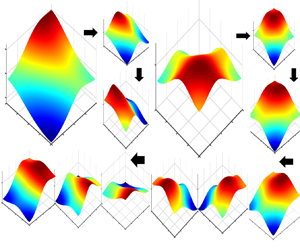
  $f_j^{(2)}(z) = \cos ({\rm \pi} j(z + 1/2)),\,j \ge 0$. Sloshing mode fi,j shows the natural mode components triggered in the surge and sway directions; f 1,0 and f 0,1 mean pure sway (z-axis) and surge (x-axis) motions, respectively, as depicted in figure 1. Under external forcing, the swirling mode occurs when the forcing frequency is close to the first natural frequency of the liquid tank. Under a pure surge or sway motion, the swirling modes, however, can be triggered by the resonant sloshing with wave breaking and tank roof impact on the free surface (Faltinsen & Timokha Reference Faltinsen and Timokha2009). For self-excited sloshing, the complex sloshing phenomenon is caused by the nonlinear interactions relating to the geometry of the tank, inlet–outlet flow directions, sloshing modes at the free surface and jet fluctuations (Saeki, Madarame & Okamoto Reference Saeki, Madarame and Okamoto2001; Hua et al. Reference Hua, Cai, Zhou and Zhang2017). Besides, once sloshing waves are triggered, the phenomenon of the complex interaction of sloshing modes at the free surface occurs. In this scenario, if the sloshing oscillation frequency is close to the first resonant frequency of the tank, resonant sloshing occurs, and it might trigger swirling modes to generate swirling waves. In this work, we only focus on the swirling waves triggered by external forcing.

Figure 1. Sketch of sloshing modes (a) f 1,0; (b) f 0,1.
In the present study, the beating swirling waves are analysed in the context of the effect of various excitation angles. The hydrodynamic forces are correlated with momentum flux-type integrals along the free surface. The momentum and angular momentum of the swirling waves are explored and analysed in detail in relation to the tank motion and types of sloshing waves. The mechanism of switching direction of swirling waves is elucidated. Section 2 introduces the equations of motion written in a moving frame of reference attached to the accelerating tank. Section 3 presents the detailed results and provides a comprehensive discussion of all phenomena found in this study. Although the governing equations incorporate excitations with six degrees of freedom, only coupled surge and sway motions are included in the present simulations. Section 4 summarizes the key conclusions.
2. Mathematical formulation
In this work, a rigid tank with an unsteady velocity and partially filled with liquid is considered. As illustrated in figure 2, the tank breadth is L, the tank width is B and d 0 is the undisturbed liquid depth.
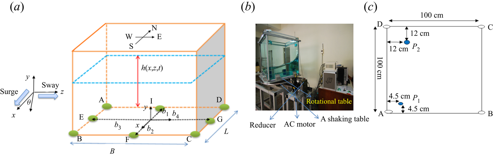
Figure 2. (a) Definition of the sketch; (b) experimental set-up; (c) positions of the wave probes from the top view of the tank.
For a tank excited at coupled surge and sway motion with the tank-fixed coordinate, the Navier–Stokes equations can be expressed as
 \begin{gather}\frac{{\partial u}}{{\partial t}} + u\frac{{\partial u}}{{\partial x}} + v\frac{{\partial u}}{{\partial y}} + w\frac{{\partial u}}{{\partial z}} ={-} \frac{1}{\rho }\frac{{\partial p}}{{\partial x}} - {\ddot{x}_C} + \upsilon {\nabla ^2}u,\end{gather}
 \begin{gather}\frac{{\partial v}}{{\partial t}} + u\frac{{\partial v}}{{\partial x}} + v\frac{{\partial v}}{{\partial y}} + w\frac{{\partial v}}{{\partial z}} ={-} g - \frac{1}{\rho }\frac{{\partial p}}{{\partial y}} + \upsilon {\nabla ^2}v,\end{gather}
 \begin{gather}\frac{{\partial w}}{{\partial t}} + u\frac{{\partial w}}{{\partial x}} + v\frac{{\partial w}}{{\partial y}} + w\frac{{\partial w}}{{\partial z}} ={-} \frac{1}{\rho }\frac{{\partial p}}{{\partial z}} - {\ddot{z}_C} + \upsilon {\nabla ^2}w,\end{gather}
where u, v and w are the liquid velocity components in the x, y and z directions relative to the tank, g is the gravitational acceleration, p is the pressure,  $\rho $ is the liquid density and $\upsilon$ is the kinematic viscosity coefficient. Further, the terms ${\ddot{x}_C}$ and ${\ddot{z}_C}$ are the acceleration components of the tank in the x- and z-directions, respectively. The continuity equation for incompressible flow is
 \begin{equation}\frac{{\partial u}}{{\partial x}} + \frac{{\partial v}}{{\partial y}} + \frac{{\partial w}}{{\partial z}} = 0.\end{equation}
The kinematic boundary condition on the free surface is
 \begin{equation}\frac{{\partial \eta }}{{\partial t}} + u\frac{{\partial \eta }}{{\partial x}} + w\frac{{\partial \eta }}{{\partial z}} = v.\end{equation}
Here,  $\eta (x,z,t) = h(x,z,t) - {d_0}$ is the wave elevation measured from the liquid surface at rest. The dynamic conditions can be expressed as follows:
 \begin{gather}{n_i}{\sigma _{ij}}{n_j} ={-} {p_{atm}} = 0,\end{gather}
 \begin{gather}{\tau _i}{\sigma _{ij}}{n_j} = 0,\end{gather}
 \begin{gather}{\sigma _{ij}} ={-} p{\delta _{ij}} + \mu \left( {\frac{{\partial {u_i}}}{{\partial {x_j}}} + \frac{{\partial {u_j}}}{{\partial {x_i}}}} \right),\end{gather}
where  ${n_i}$ and ${\tau _i}$ are the normal and tangential unit vectors to the free surface, and ${\sigma _{ij}}$ is the ith component of the stress tensor acting on the surface. Also, ${\delta _{ij}}$ is the Kronecker delta. The no-slip condition is applied at the boundary between the liquid and the tank surface except at the intersection line between the free surface and the tank surface. For the initial condition, all parameters implemented in the study are set to zero at the beginning of the simulations.
In the present study, we employ simple mapping functions to remove the time dependence of the free surface in the fluid domain. The irregular boundary, including the time-varying fluid surface, non-vertical walls and non-horizontal bottom, can be mapped onto a cubic coordinates  $({x^\ast },{y^\ast },{z^\ast })$ by the proper coordinate transformations (Hung & Wang Reference Hung and Wang1987; Chen & Nokes Reference Chen and Nokes2005). In this work, the coordinates $({x^\ast },{y^\ast },{z^\ast })$ can be further transformed such that the layers near the wall and free surface boundaries are stretched to capture sharp local velocity gradients and free surface profile. The above governing equations were solved in dimensionless forms. The detailed coordinate transformation and the dimensionless equations implemented in the study are tedious and have already been reported in Wu & Chen (Reference Wu and Chen2009). The Crank–Nicholson second-order finite-difference scheme and the Gauss–Seidel point successive overrelaxation iterative procedure are implemented to calculate fluid velocity and pressure, respectively. The detailed finite-difference method can be found in Appendix A and also in Wu (Reference Wu2009).
3. Results and discussion
The convergence study of the present numerical model was extensively validated in the reported papers (Wu & Chen Reference Wu, Faltinsen and Chen2009; Wu et al. Reference Wu, Chen and Hung2013). Figure 3 compares the wave elevations at probe 1 (HA: wave elevation at probe 1) and probe 2 (HD: wave elevation at probe 2) of swirling waves at θ = 15°. The agreements of the comparison are very good, and more numerical validation can be found in Wu (Reference Wu2009) and Wu et al. (Reference Wu, Chen and Hung2013). The tank size of the following simulations is fixed as B/L = 1. Based on the definition of the excitation angle θ, the components of the excitation amplitude in surge (x-axis) and sway (z-axis) directions are  ${a_0}\sin ({\omega _f}t)\cos (\theta )$ and ${a_0}\sin ({\omega _f}t)\sin (\theta )$, respectively, where a 0 is the excitation amplitude of the tank and ωf is the external forcing frequency. The numerical and experimental results show an excellent agreement. The phenomenon of switching of the direction of swirling waves was also observed in the experiment, which will be elucidated in this study.

Figure 3. Comparison between the present results of experiment and numerical simulation. The measured data at (a) wave probe P 1; (b) wave probe P 2; T = 0–60 s, B/L = 1, d 0/L = 0.25, a 0/L = 0.005, ωf = 0.97ω 1,0, θ = 15°.
3.1. Beating phenomenon with various excitation angles
The sloshing amplitude function is a combination of an amplitude-modulated harmonic function with a frequency equal to the difference of the forced frequency (ωf) and the fundamental frequency of liquid in tank (ω 1) and the amplitude varying with a frequency of sum of ωf and ω 1. For a tank under harmonic excitation, the sloshing amplitude function may have a factor of  $(\cos ({\omega _f}t)-\cos ({\omega _0}t))$ or $\sin (({\omega _0}-{\omega _f})t/2)\sin (({\omega _0} + {\omega _f}) t/2)$. If the natural and forced frequencies are similar, i.e. $|{\omega _0}-{\omega _f}|$ is small, then the amplitude function is a low-frequency function multiplying a high-frequency function. This phenomenon is known as beating. The ‘beating’ phenomenon of swirling waves is well known from experimental studies on sloshing motions in circular and spherical tanks. In particular, Abramson (Reference Abramson1966, p. 99) noted: ‘The motion is even more complicated as a type of “beating” also exists; the first anti-symmetric liquid-sloshing mode first begins to transform itself into a rotational motion increasing in angular velocity in, say, the counterclockwise direction, which reaches a maximum and then decreases essentially to zero and then reverses and increases in the clockwise direction, and so on alternatively’.
The swirling waves only occur within a range of excitation frequencies close to the resonant excitations, and swirling behaviour is seldom seen when the excitation angle θ is larger than 30° or close to 0°. Figure 4 depicts the wave history of HA with various excitation angles and shows different beating periods of sloshing waves. The dimensionless time T is defined as  $T = t\sqrt {g/{d_0}} $. The first beating period of point A (HA) increases as does the excitation angle. Besides, the distinct first beating period of swirling waves at various excitation angles may stem from the effect of wave nonlinearity, which is defined as the ratio of wave elevation of the maximum peak ηmax to the maximum trough ηmin. The nonlinearity of wave elevations of θ = 5°, 10°, 15° and 30° is 2.265, 2.312, 2.464 and 3.196, respectively, which increases with the excitation angle. The nonlinearity is also correlated deeply with water depth, excitation amplitude and excitation frequency of the tank. For more investigations of wave nonlinearity the reader referred to Wu et al. (Reference Wu, Chen and Hung2013).

Figure 4. Wave history (HA) of swirling waves with various excitation angles; d 0/L = 0.25, a 0/L = 0.005, ωf = 0.97ω 1,0. Solid line: θ = 5°; dash line: θ = 10°; dotted line: θ = 15°; dash-dotted line: θ = 30°.
3.2. Flow momentum and angular momentum of swirling waves
Physically, the circulatory flow motion in the tank can be correlated with the fluid momentum in the x and z axes. The dimensionless horizontal momentum of the fluid (Mo) in the tank can be obtained by
 \begin{equation}Mo = {{\left( {\rho \left[ {\iint\!\!\!\int {{u_a}\,\textrm{d}\kern0.06em x\,\textrm{d}y\,\textrm{d}z} + \iint\!\!\!\int {{w_a}\,\textrm{d}\kern0.06em x\,\textrm{d}y\,\textrm{d}z} } \right]} \right)} / {\rho \sqrt {g{d_0}} d_0^3}} = M{o_x} + M{o_z},\end{equation}
where Mox and Moz are the components of the fluid momentum contributed by velocity components ua and wa (global system), respectively. To investigate the rotation of swirling waves, we further define the angular momentum of the circulatory flow to the x, y and z axes in the tank, respectively, as
 \begin{gather}{M_{\theta x}} = {{\left( {\rho \left[ {\iint\!\!\!\int {{w_a}\,\textrm{d}\kern0.06em x\,\textrm{d}y\,\textrm{d}z} \times {r_y} + \iint\!\!\!\int {{v_a}\,\textrm{d}\kern0.06em x\,\textrm{d}y\,\textrm{d}z \times {r_z}} } \right]} \right)} / {\rho \sqrt {g{d_0}} d_0^4}},\end{gather}
 \begin{gather}{M_{\theta y}} = {{\left( {\rho \left[ {\iint\!\!\!\int {{u_a}\,\textrm{d}\kern0.06em x\,\textrm{d}y\,\textrm{d}z} \times {r_z} + \iint\!\!\!\int {{w_a}\,\textrm{d}\kern0.06em x\,\textrm{d}y\,\textrm{d}z \times {r_x}} } \right]} \right)} / {\rho \sqrt {g{d_0}} d_0^4}},\end{gather}
 \begin{gather}{M_{\theta z}} = {{\left( {\rho \left[ {\iint\!\!\!\int {{u_a}\,\textrm{d}\kern0.06em x\,\textrm{d}y\,\textrm{d}z} \times {r_y} + \iint\!\!\!\int {{v_a}\,\textrm{d}\kern0.06em x\,\textrm{d}y\,\textrm{d}z \times {r_x}} } \right]} \right)} / {\rho \sqrt {g{d_0}} d_0^4}},\end{gather}
where r is the horizontal distance from the tank centre to the position of the liquid element and the subscript of r is the direction to the designated axis. The swirling direction of the sloshing waves is presented by Mθy. The rate of change of angular momentum at a fixed reference point is equal to the external forces (moments) acting on the body. In other words, the external forces acting on the tank are transferred to the rate of change of angular momentum of fluid particles in the tank. The rate of change of angular momentum of sloshing waves (MT) about the tank centre, therefore, is equal to the external moments acting on the tank
 \begin{align}
{M_T} & = \dfrac{{\textrm{d}{M_{\theta y}}}}{{\textrm{d}t}}
= {{\left( {\rho \left[ {\iint\!\!\!\int
{\dfrac{{\textrm{d}{u_a}}}{{\textrm{d}t}}\,\textrm{d}\kern0.06em
x\,\textrm{d}y\,\textrm{d}z} \times {r_z} + \iint\!\!\!\int
{\dfrac{{\textrm{d}{w_a}}}{{\textrm{d}t}}\,\textrm{d}\kern0.06em
x\,\textrm{d}y\,\textrm{d}z \times {r_x}} } \right]}
\right)} / {\rho gd_0^4}}\\ & = \sum {r \times {F_{ext}}} .
\end{align}
\begin{align}
{M_T} & = \dfrac{{\textrm{d}{M_{\theta y}}}}{{\textrm{d}t}}
= {{\left( {\rho \left[ {\iint\!\!\!\int
{\dfrac{{\textrm{d}{u_a}}}{{\textrm{d}t}}\,\textrm{d}\kern0.06em
x\,\textrm{d}y\,\textrm{d}z} \times {r_z} + \iint\!\!\!\int
{\dfrac{{\textrm{d}{w_a}}}{{\textrm{d}t}}\,\textrm{d}\kern0.06em
x\,\textrm{d}y\,\textrm{d}z \times {r_x}} } \right]}
\right)} / {\rho gd_0^4}}\\ & = \sum {r \times {F_{ext}}} .
\end{align}
Angular moment Mθy tells the direction and strength of the swirling waves. We, therefore, only consider the rate of change of angular momentum in the y-axis. In this study, we define the positive and negative MT as indicating, respectively, the counterclockwise and clockwise moments acting on the fluid by the external forcing. Figure 5 shows the time histories of the momentum of the flow and the wave elevation at point A. The total energy of sloshing waves is a combination of kinetic energy and potential energy. The maximum kinetic energy of the waves appears when the free surface is nearly flat. The peaks of Mox and Moz occur at HA close to 0. Oppositely, as Mox and Moz are almost zero and, therefore, the peaks of HA are presented.

Figure 5. Momentum of the waves in the x-direction (Mox: solid line) and in the z-direction (Moz: dash line) and the dimensionless elevation (HA): dotted line; d 0/L = 0.25, a 0/L = 0.005, ωf = 0.97ω 1,0, θ = 15°.
The momentum of the liquid in the tank is deeply correlated with the tank motion. As illustrated in figure 6, the motion of the tank (dotted line) will cause the liquid to move in the opposite direction to the tank motion due to the inertial effect. In other words, the forward tank motion (figure 6a, see time interval from point A to point B) results in the tendency of the backward movement of the liquid and, therefore, the original forward movement of the fluid (Mox and Moz > 0) is gradually influenced by the tank motion and then turns into the backward motion at T = 17.5 (Mox and Moz < 0). The inverse phenomenon is shown when the tank motion becomes backward (see the time interval from point B to point C). Since an inclined excitation (θ = 15°) was applied, Mox is initially larger than Moz. This indicates that the flow in the tank moves faster in the North–South direction than in the East–West direction. The phenomenon of flow motion is opposite when Mox < Moz. Besides, the travel direction of the flow in the tank can be estimated by the phase difference between Mox and Moz. As depicted in figure 6(b), the phases of Mox and Moz are almost identical during T = 0 ~ 40. This means the flow motion in the tank is travelling in a constant back-and-forth direction, referred to as ‘single-directional’ waves (Chen & Wu Reference Chen and Wu2011). It is known that swirling motion occurs due to the simultaneous appearance of the f (1,0) and f (0,1) modes and their phase angles have some differences. That is, as the phase lag between Mox and Moz occurs, the direction of flow motion is no longer fixed, it is varied with time instead and then the circulatory flow (swirling waves) appears. The envelope of the liquid momentum increases with time (T = 0 ~ 100) as well as the strength of the flow motion inside the tank. After T > 100, the peaks of Mox decrease with time, whereas the peaks of Moz continually increase. As T = 155 ~ 165, the phase lag between Mox and Moz nearly disappears and the magnitudes of Mox and Moz are almost equal. In other words, a nearly diagonal wave appears during this period (T = 155–165). The reason the strength of the swirling waves is reduced and replaced by the diagonal-like waves can be associated with the tank motion and the fluid momentum Mox. The swirling waves occur when T > 40, the circulatory flow motion in the tank has its own oscillating period and the flow motion in the tank is no longer dominated by the tank motion. The phase difference between Mox and the tank motion gradually becomes apparent. When the phase lag of Mox is approximately 1/4 period later than that of the tank motion (see point D to point E), the forward tank motion encounters the instantaneous backward flow movement in the surge direction (Mox < 0). The strength of swirling waves gradually reduces to zero and the sloshing wave turns into a single-directional wave. In short, the evolution of sloshing waves during the first beating period includes single-directional waves (T = 0 ~ 40) → counterclockwise swirling waves (T = 40 ~ 155) → nearly single-directional waves (T = 155 ~ 165)→ clockwise swirling waves (T > 170).

Figure 6. Momentum of the waves in the x direction (Mox: solid line) and in the z-direction (Moz: dash line) and the dimensionless excitation displacement of the tank (a 0/d 0): dotted line; d 0/L = 0.25, a 0/L = 0.005, ωf = 0.97ω 1,0, θ = 15°.
3.3. The switch of swirling directions
Faltinsen et al. (Reference Faltinsen, Rognebakke and Timokha2005) indicated ‘The switching of the rotational direction of swirling waves was most probably affected by random perturbations occurring due to the local phenomena including the steepness of the wave pattern and local breaking phenomena’. However, the detailed physical mechanism by which the switching direction of swirling waves is still not clear.
Figure 7 portrays the time histories of the components of angular momentum (Mθ) of the liquid in the tank; Mθy presents the swirling direction of the waves, and positive and negative Mθy indicate counterclockwise and clockwise flow motions, respectively. As depicted in figure 7(a), Mθy apparently increases after T = 40, and so does the strength of counterclockwise swirling waves. At T = 170, Mθy decreases to become negative and the swirling wave switches from counterclockwise to clockwise. From T = 0 to 1380, there are five switches. As illustrated in figure 7(b), we found that the swirling direction switches from counterclockwise to clockwise when Mθx and Mθz are out of phase (mode (1,0), f (1,0), is dominant) and it switches from clockwise to counterclockwise when Mθx and Mθz are in phase (mode (0,1), f (0,1), is dominant). Besides, at the moment of switching direction, Mθx, Mθy and Mθz are all close to 0. In other words, the sloshing waves become nearly single-directional waves at the time of switch.

Figure 7. Angular momentum Mθ of swirling waves: (a) Mθx and Mθy; (b) swirling wave switch from counterclockwise to clockwise when Mθx and Mθz are out of phase; switch from clockwise to counter-clockwise when Mθx and Mθz are in phase; (c,d) zoom in of the circular parts of (b); d 0/L = 0.25, a 0/L = 0.005, ωf = 0.97ω 1,0, θ = 15°.
Based on the momentum balance (Wu et al. Reference Wu, Chen and Hung2013), the velocity component ‘w’ is mainly generated by external forcing components in the z-axis and can be represented by sloshing-induced force in the z direction (Fz)
 \begin{equation}{F_z} = {{\left[ {\int_{ - L/2}^{L/2} {\int_0^h {{P_W}\,\textrm{d}y\,\textrm{d}\kern0.06em x} } + \int_{ - L/2}^{L/2} {\int_0^h {{P_E}\,\textrm{d}y\,\textrm{d}\kern0.06em x} } } \right]} / {\rho gd_0^3}},\end{equation}
in which the subscripts E and W represent the pressure integrations on the east and west walls of the tank. The beating phenomenon can be found in the time history of Fz shown in figure 8 and we can connect each peak and trough of Fz for generating Fz-envelope. As depicted in figure 8, the counterclockwise swirling wave occurs as Fz increases, whereas the clockwise swirling wave appears as Fz decreases during each swirling period. At the peak and trough of Fz-envelope, the single-directional waves and the switch occur. Similar behaviours were found (figure 9) in the varied cases with different excitation angles and frequencies.

Figure 8. Horizontal sloshing-induced force component Fz; d 0/L = 0.25, a 0/L = 0.005, ωf = 0.97ω 1,0 and θ = 15°. The switch direction from counterclockwise to clockwise always occurs at Fz-peak, whereas and the switch direction from clockwise to counterclockwise always occurs at Fz-trough.

Figure 9. Angular momentum components, Mθy, of swirling waves: (a) ωf = 1.05ω 1,0, θ = 10°; (b) ωf = 0.95ω 1,0, θ = 30°; d 0/L = 0.25, a 0/L = 0.005.
The question remains: Why is the swirling period of the sloshing wave related to the sloshing-induced force Fz? This can be found from the effect of the secondary mode. As the excitation angle is close to 0, the swirling wave is hard to generate unless by the influence of some other disturbances, such as breaking waves. As the excitation angle increases, the tank motion has two components which can be divided into primary and secondary components. For θ = 15°, the primary and secondary components are in the x (surge) and z (sway) directions, respectively. The primary component of tank motion excites fluid sloshing, while the secondary component of tank motion is to trigger swirling flow. As a result, the swirling period of the wave is almost identical to that of the z-component of induced force Fz, which is attributed to the secondary component of tank excitation.
In addition, the beating period of Fz can be used to estimate the swirling period of the waves. Since Fz is related to the secondary tank motion, its beating period can be approximately calculated by the 2-D beating wave period from an analytic solution
 \begin{equation}{T_a} = 2{\rm \pi}/(|{\omega _f}-{\omega _1}|)\times \sqrt {g/{d_0}} ,\end{equation}
where ωf and ω 1 are, respectively, the excitation frequency and the first natural frequency of liquid in tank. The mean value of the swirling period (up to T = 1500) was compared with the analytic solution, as shown in figure 10. The difference between our simulated results and the analytical solution is less than 10 % and the empirical swirling period of sloshing wave (Ts) may be expressed as
 \begin{equation}{T_s} = (1 \pm 0.1)\times
2{\rm \pi}/(|{\omega _f}-{\omega _1}|)\times \sqrt {g/{d_0}}.\end{equation}
\begin{equation}{T_s} = (1 \pm 0.1)\times
2{\rm \pi}/(|{\omega _f}-{\omega _1}|)\times \sqrt {g/{d_0}}.\end{equation}
As excitation angle θ increases, the difference between Ta and Ts increases as well, which is related to sloshing nonlinearity due to various excitation angles (Chen & Wu Reference Chen and Wu2011).

Figure 10. Comparison of dimensionless swirling period of waves between the analytic result and the present simulations; d 0/L = 0.25, a 0/L = 0.005.
As mentioned earlier, tank displacement plays an important role in increasing or decreasing the liquid momentum (MO) and liquid angular momentum (Mθ). The rate change of angular momentum (MT) is equal to the sum of the external force moments acting on the fluid in the tank, as shown in (3.5). According to the definition direction of angular momentum Mθy in this study, MT > 0 means that the external forcing moment triggers counterclockwise moments to the fluid inside the tank. On the other hand, the clockwise moment of the fluid was triggered by the external forcing moment when MT < 0. Figure 11 depicts the time history of MT of the swirling waves and the associated variation of Mθy. As T < 120, MT is positive, the external forcing generates a counterclockwise moment to the fluid, which results in the increase of Mθy; Mθy gradually diminishes as T > 120 and the strength of counterclockwise flow is reduced because the external forcing induces clockwise moments (MT < 0) to the fluid. As the counterclockwise flow strength decreases to almost 0 (Mθy ~ 0), there is no circulatory flow in the tank. As a result, single-directional waves occur. The external forcing moment varies the flow circulation strength and direction, and the switch between swirling and single-directional waves occurs. At T = 170, Mθy becomes negative and swirling flow changes to clockwise flow. As T > 200, the dominant moment induced by external forcing becomes counterclockwise (MT > 0), which reduces the strength of the clockwise flow. Afterwards, the clockwise swirling wave shifts its direction to the counterclockwise direction (Mθy > 0) at T ~ 270. We clearly found that the external excitation forcing affects the strength of the swirling motion of the fluid in the tank.

Figure 11. The rate of change of angular momentum (MT), and we can see how MT (dark line) affects the increase and decrease of Mθy (orange line) and switches swirling direction; d 0/L = 0.25, a 0/L = 0.005, ωf = 0.97ω 1,0, θ = 15°.
Figure 12 demonstrates one of the switch point occurring at the peak of Fz-envelope at which Mθx and Mθz are out of phase (figure 7b). At the time, Mθx-envelope is at its peak, which implies the single-direction wave is primarily attributed to f (1,0) and the trajectory of the mass centre is biased towards the surge direction (see snapshots). The other switch point occurs at the trough of Fz-envelope at which Mθx-envelope is at its trough and f (0,1) has more effect than f (1,0) on the single-direction wave and the trajectory of the mass centre is biased more towards the sway direction. As an example, at T = 395.9 to 401.63, the trajectory of the flow mass centre is in a South–Westerly direction and, at the same time, the tank is moving in the South–East direction and the inertia (gravitational) effect results in switching of the swirling direction to a clockwise direction. Oppositely, at T = 521.16 to 526.62, the trajectory of the flow mass centre is moving North–Easterly and the instantaneous tank motion results in switching of the swirling direction to a counterclockwise direction. The movie of the phenomena mentioned above for swirling waves is provided as supplementary material (available at https://doi.org/10.1017/jfm.2022.896).

Figure 12. (a) Single-directional waves always occur at the peak and trough of Fz-envelope (snapshots: arrow sign in blue colour indicates the tank motion direction, arrow sign in green colour indicates the trajectory of mass volume centre); (b) snapshots of clockwise swirling waves (upper subplot in sequential order 1→2→3→4) and counterclockwise swirling waves (lower subplot in sequential order 1→2→3→4).
3.4. Frequency domain of swirling waves
The frequency domain of swirling waves would be good information to estimate the occurrence of the swirling phenomenon. We simulated more cases at various excitation angles, excitation amplitudes and water depths to find the frequency range of swirling waves and the result is depicted in figure 13. The results of Faltinsen & Timokha (Reference Faltinsen and Timokha2009) are also shown in the figure, their results are, however, limited to a fixed excitation direction (i.e. in the surge direction). As the tank has a shallow liquid depth, the frequency domain of swirling waves becomes wider, especially for a tank exited with a larger excitation amplitude (a 0/L = 0.0078). On the contrary, the frequency domain of swirling waves is limited to a small range for the tank with finite liquid depths. The corresponding maximum sloshing amplitudes (ηmax) of the cases of  $\theta = 10\mathrm{^\circ }$ and 30° in figure 13 are depicted in figure 14, and the wave nonlinearity $\textrm{(}{\eta _{max}}/{\eta _{min}}\textrm{)}\ \textrm{at}\ \theta = 30\mathrm{^\circ }$ is illustrated in figure 15. According to the assumption of the proposed numerical model, we cannot consider the phenomena of wave breaking, wave run-up and tank roof impact in the simulations. In other words, ηmax is captured before the simulation diverges at nearly resonant sloshing. In figure 14, the soft-spring and hard-spring responses of ηmax are presented near the first resonant excitation frequency (ω 1,0) in a shallow liquid (d 0/L ≤ 0.25) and at finite liquid depths (d 0/L ≥ 0.4), respectively. In addition, the effect of excitation angle on ηmax is more significant as the liquid depth decreases, especially for the shallow liquid depth. Increasing the excitation amplitude (a 0/L = 0.0078) of the tank results in larger ηmax and sloshing nonlinearity (figure 15). As the liquid depth decreases from the finite to shallow depths, the nonlinearity of sloshing waves increases significantly. As we know, the wave travel speed decreases with the liquid depth. The increased nonlinearity of sloshing waves diminishes the travel speed of sloshing waves resulting in the hysteresis phenomenon on the resonant frequency (ω 1,0) in shallow liquid depths. Thus, the soft-spring phenomenon is presented for shallow water depths.

Figure 13. The frequency domain of swirling waves under various water depths, excitation angles and excitation amplitudes.

Figure 14. Maximum sloshing amplitude under various water depths, excitation angles and excitation amplitudes; (a) a 0/L = 0.005; (b) a 0/L = 0.0078.

Figure 15. Nonlinearity of sloshing waves under different water depths and excitation amplitudes; θ = 30°.
The effect of excitation angle on the shift of the frequency domain of swirling waves is clearly seen by comparing with the results of Faltinsen & Timokha (Reference Faltinsen and Timokha2009) for a tank under 0-degree excitation (surge motion). Although different beat periods and sloshing displacements of swirling waves are presented due to the effect of excitation angle, the corresponding frequency domains are nearly the same when the excitation angle is in the range of 5° ≤ θ < 30°. The frequency domain of swirling waves slightly reduces as θ = 30°, which might be caused by the effect of the nonlinearity of sloshing waves. In short, the evolutions of swirling waves are very sensitive to physical conditions, including liquid depth, excitation angle, excitation amplitude and frequency of external forcing.
4. Conclusion
The sloshing displacement of liquid in a tank is a combination of the standing wave and forced (progressive) wave. When a 3-D tank is under a near-resonant excitation, the beat phenomenon occurs, and a secondary excitation force creates swirling flow. In our study, the following concluding remarks can be given:
(i) The period of a swirling wave in a tank is closely related to the beat period, while the swirling behaviour is seldom seen when θ is larger than 30° or close to 0°. The oblique excitation produces two excitation components and the secondary component triggers rotational waves.
(ii) The excitation moment enhances or reduces the circulation strength, and the instantaneous tank motion finally switches the circulation direction. The magnitude of the components of liquid angular momentum, Mθx and Mθz, and their phase difference are the key factors in determining the quantity of fluid movement and the direction of the circulatory flow.
(iii) Further, the phase difference between the tank motion and the fluid momentum is significant in influencing the strength of the circulatory flow. The angular momentum of the liquid Mθy represents the strength and the rotational direction of the circulatory flow in the tank. The sum of the moment made by an external force acting on the fluid is equal to the rate of change of angular momentum of the fluid, and plays an important role in affecting the strength of rotation of swirling waves.
(iv) The evolutions of swirling waves are very sensitive to physical conditions, including liquid depth, excitation angle, excitation amplitude and frequency of external forcing.
(v) The switch of the swirling direction always occurs at the peak or trough of Fz-envelope. The external excitation moment varies the circulation strength, and the swirling wave becomes a single-directional wave, but it is only sustained for a short period of time. The instantaneous tank motion at the time finally switches the consequent circulation direction.
Supplementary movie
Supplementary movie is available at https://doi.org/10.1017/jfm.2022.896.
Funding
The study is partially supported by National Science and Technology Council of Taiwan under a grant 109-2221-E-110-025-MY2.
Declaration of interests
The authors report no conflict of interest.
Author contributions
B.-F.C. and O.M.F. derived the theory; C.-H.W. performed the simulations, B.-F.C. and C.-H.W. contributed equally to analysing data, reaching conclusions and writing the paper.
Appendix A. Numerical method used in this study
A.1. Coordinate transformation
Accurate free surface tracking of sloshing in tanks is an important factor for many numerical methods, especially when sloshing nonlinearity is significant. Among these methods, σ-transformation (Frandsen Reference Frandsen2004), marker and cell, VOF, smoothed-particle hydrodynamics (SPH) and the level set method (LSM) are frequently used in treating time-varying free surface flow. For violent sloshing, wave breaking might be captured by VOF, LSM and SPH. However, the prediction of energy dissipation due to wave breaking and conservation of fluid mass among these methods still needs to be improved. In the present study, we employ simple mapping functions to remove the time dependence of the free surface in the fluid domain. The irregular boundary, including the time-varying fluid surface, non-vertical walls and non-horizontal bottom, can be mapped onto a cube by the proper coordinate transformations (Hung & Wang Reference Hung and Wang1987; Chen & Nokes Reference Chen and Nokes2005; Wu et al. Reference Wu, Chen and Hung2013)
 \begin{equation}{x^\ast } = \frac{{x - {b_1}(y,z)}}{{{b_2}(y,z) - {b_1}(y,z)}},\quad {y^\ast } = \frac{{y + d(x,z)}}{{h(x,z,t)}},\quad {z^\ast } = \frac{{z - {b_3}(x,y)}}{{{b_4}(x,y) - {b_3}(x,y)}},\end{equation}
where the instantaneous water depth,  $h(x,z,t)$, is a single-valued function measured from the tank bottom, d (x,z) represents the vertical distance between the still water surface and the tank bottom, b 1 and b 2 are horizontal distances from the z-axis to the south and north walls, respectively, and b 3 and b 4 are horizontal distances from the x-axis to the west and east walls, respectively (see figure 2). Through (A1), one can map the north wall to ${x^\ast } = 0$ and south wall to ${x^\ast } = 1$, the west wall to ${z^\ast } = 0$ and east wall to ${z^\ast } = 1$, the tank bottom to ${y^\ast } = 0$ and the free surface to ${y^\ast } = 1$. The main advantage of these transformations is to map a wavy and time-dependent fluid domain onto a time-independent unit cubic domain, which makes the program coding more efficient. In addition, re-meshing due to the wavy free surface is unnecessary and the mapping implicitly deals with the free surface motion and avoids the need to calculate the free surface velocity components explicitly. Extrapolations are unnecessary and free surface smoothing by means of a spatial filter is not required. All calculations can be done under a time-independent computational domain due to the consequence of coordinate transformation. However, the phenomena of wave breaking, run-up and tank roof impacts are not considered in the present study based on the assumption of $h(x,z,t)$. Unlike VOF and LSM, which solve two phase flow (air and water), the present numerical model only considers one phase (water). Thus, the computational time can be reduced.
For resonant sloshing, before wave breaking, very steep waves might occur at rigid walls of the container. The coordinate system becomes far from orthogonal, resulting in inaccuracy of discretization. In this work, the coordinates  $({x^\ast },{y^\ast },{z^\ast })$ can be further transformed such that the layers near the wall and free surface boundaries are stretched to capture sharp local velocity gradients and the free surface profile. The following exponential functions provide these stretching transformations:
 \begin{align}X &= {\lambda _1} + ({x^\ast } - {\lambda _1})\,{\textrm{e}^{{k_1}{x^\ast }({x^\ast } - 1)}},\quad Y = {\lambda _2} + ({y^\ast } - {\lambda _2})\,{\textrm{e}^{{k_2}{y^\ast }({y^\ast } - 1)}},\nonumber\\ Z &= {\lambda _3} + ({z^\ast } - {\lambda _3})\,{\textrm{e}^{{k_3}{z^\ast }({z^\ast } - 1)}}.\end{align}
The constants  ${k_i}$ and ${\lambda _i}(i = 1,2,3)$ control the mesh size and stretching in the X-, Y- and Z- directions, respectively. The parametric study of constants ${k_i}$ and ${\lambda _i}$ has been performed by Wu & Chen (Reference Wu and Chen2009) to accurately capture the free surface profile near the tank walls for resonant sloshing. As a result, the same constants ( $\lambda_1 = \lambda_2 =\lambda_3 = 0.5$ and $k_1 = k_2 = k_3 = 2$) are used in the present study as well, and the stretching grid is depicted in Wu & Chen (Reference Wu and Chen2009). However, the assumption of a single-valued free surface still has limitations in predicting sloshing, particularly when a shallow water depth with highly nonlinear sloshing is considered. Based on the authors’ experiences, the approximate limitation of the present scheme under near-resonant excitations (0.97ω 1, ω 1: the first natural frequency mode) is determined when a 0 (excitation amplitude)/d 0 is close to 0.1 in the shallow liquid depth (d 0/L = 0.1) case. For non-resonant excitations, it seems to be able to tolerate much larger excitation amplitudes (a 0/d 0 > 2.5) for the present numerical approach.
The dimensional parameters are normalized as follows:
 \begin{equation}\left. {\begin{array}{*{20}{c}} {U = \dfrac{u}{{\sqrt {g{d_0}} }},\quad V = \dfrac{v}{{\sqrt {g{d_0}} }},\quad W = \dfrac{w}{{\sqrt {g{d_0}} }},\quad P = \dfrac{p}{{\rho g{d_0}}},\quad T = t\sqrt {\dfrac{g}{{{d_0}}}} ,}\\ {H = \dfrac{\eta }{{{d_0}}},\quad {{\ddot{X}}_c} = {{\ddot{x}}_c}/g,\quad {Z_c} = {{\ddot{z}}_c}/g.} \end{array}} \right\}\end{equation}
The detailed dimensionless equations implemented in the study are tedious and have already been reported by Wu et al. (Reference Wu, Chen and Hung2013) and, therefore, are omitted in the text.
A.2. Computational algorithm
A.2.1. Finite-difference method
In the present 3-D analysis, the finite-difference method is used to discretize the dimensionless equations in the transformed X-Y-Z coordinate system. Central difference approximation is used for the space derivatives in the fluid domain, except at the boundary, where forward or backward differences are employed. By employing a staggered grid system, the pressure P is defined at the centre of a finite-difference grid cell (of dimensions $(\Delta X,\Delta Y,\Delta Z)$), whereas the velocity components U, V and W are calculated $0.5\Delta X$, $0.5\Delta Y$ and $0.5\Delta Z$ behind, above or backward of the cell centre. The free surface elevation H is at the same location as that of vertical velocity V.
The Crank–Nicholson second-order finite-difference scheme and the Gauss–Seidel point successive overrelaxation iterative procedure are implemented to calculate fluid velocity and pressure, respectively. When the dimensionless equations (Chen & Wu Reference Chen and Wu2011) are set to be balanced at time  $T = (n + 1/2)\Delta T$, the finite-difference forms of them are
 \begin{gather}U_{i,j,k}^{n + 1} = U_{i,j,k}^n - \Delta T({\wp _{i,j,k}} + P_{i,j,k}^X),\end{gather}
 \begin{gather}V_{i,j,k}^{n + 1} = V_{i,j,k}^n - \Delta T({{\rm Re} _{i,j,k}} + P_{i,j,k}^Y),\end{gather}
 \begin{gather}W_{i,j,k}^{n + 1} = W_{i,j,k}^n - \Delta T({\aleph _{i,j,k}} + P_{i,j,k}^Z),\end{gather}
 \begin{gather}H_{i,j,k}^{n + 1} = H_{i,j,k}^n - \Delta T({{\rm Im} _{i,j,k}} + {V_{i,j,k}}).\end{gather}
In these equations, the superscript n represents the time index (i.e.  $T = n\Delta T$) and ΔT is the dimensionless time step. The terms without a superscript are at $T = (n + 1/2)\Delta T$. The velocity components at $T = (n + 1/2)\Delta T$ can be approximated as the averages of the values at $n\Delta T$ and $(n + 1)\Delta T$. All of the terms on the right-hand side of (A4)–(A6) are applied at the same nodes as ${U_{i,j,k}},{V_{i,j,k}}$ and ${W_{i,j,k}}$. The terms $P_{i,j,k}^X,P_{i,j,k}^Y$ and $P_{i,j,k}^Z$ are the corresponding pressure gradients in the X, Y and Z directions, respectively. The terms ${\wp _{i,j,k}}$, ${{\rm Re} _{i,j,k}}$ and ${\aleph _{i,j,k}}$ contain all of the remaining terms in the dimensionless equations (Wu Reference Wu2009) grouped together, including the finite-difference expressions for the convective acceleration, diffusive terms and the terms related to tank motion. In (A7), ${{\rm Im} _{i,j,k}}$ is the nonlinear term of pressure wave equation. The pressure is evaluated by solving the Poisson equation. For $T = (n + 1/2)\Delta T$, one can express the finite-difference equation in the following form:
 \begin{equation}{P_{i,j,k}} = \varPsi \left[ {\frac{1}{{{a_{i,j,k}}}}({\varPi_{i,j,k}} + {\varOmega_{i,j,k}}) + P_{i,j,k}^\ast } \right] + (1 - \varPsi )P_{i,j,k}^\ast ,\end{equation}
in which  ${a_{i,j,k}}$ is the sum of the coefficients of pressure ${P_{i,j,k}}$, $\varPsi $ is the relaxation parameter and $P_{i,j,k}^\ast $ is the previously iterated pressure. The relaxation parameter $\varPsi $ is chosen to be 0.7 in the present study based on previous works (Wu et al. Reference Wu, Faltinsen and Chen2012). The terms ${\varPi _{i,j,k}}$ represent the finite-difference expressions of the pressure gradient and ${\varOmega _{i,j,k}}$ the finite-difference expressions of the nonlinear convective accelerations and the term related to tank motion. The superscript $(n + 1/2)$, for ${P_{i,j,k}}$, ${\varPi _{i,j,k}}$ and ${\varOmega _{i,j,k}}$ is also omitted here. The detailed finite-difference expressions for ${P_{i,j,k}}$, ${\varPi _{i,j,k}}$ and ${\varOmega _{i,j,k}}$ are tedious, and are, therefore, omitted from the text. Once the pressure field has been solved by iteration, the velocity components $U_{i,j,k}^{n + 1}$, $V_{i,j,k}^{n + 1}$ and $W_{i,j,k}^{n + 1}$ can be calculated from equations, (A4)–(A6). The instantaneous water surface profile $H_{i,j,k}^{n + 1}$ can be calculated from (A7). Furthermore, we employed a second-order upwind scheme (Hirt, Nicholas & Romero Reference Hirt, Nicholas and Romero1975) in the present numerical scheme to deal with the convective terms.
In general, the errors in the solution of finite-difference equations may be caused by round-off error, which is a property of the computer, or by the application of a particular numerical method, i.e. a discretization error. If the errors introduced into the finite-difference equation (FDE) are not controlled, the growth of errors with the solution of the FDE will result in an unstable solution. The accuracy of the numerical results significantly depends on the spatial grid resolution and the selected time step. The present simulation time step and grid size are restricted by the condition given in (A9)
 \begin{equation}\left. {\begin{array}{*{20}{c@{}}} {\Delta t < min\left\{ {\dfrac{{\Delta {x_{min}}}}{{|{u_{i,j,k}}|}},\dfrac{{\Delta {y_{min}}}}{{|{v_{i,j,k}}|}},\dfrac{{\Delta {z_{min}}}}{{|{w_{i,j,k}}|}}} \right\}}\\ {v\Delta t < \dfrac{1}{2}\dfrac{{\Delta x_{min}^2\Delta y_{min}^2\Delta z_{min}^2}}{{\Delta x_{min}^2 + \Delta y_{min}^2 + \Delta z_{min}^2}}} \end{array}} \right\}.\end{equation}
Equation (A9) implies that a liquid particle cannot move more than one cell in a single time step and the diffusion of momentum is not significant over more than one cell in one time step.
A.2.2. Iterative procedures
The finite-difference equations mentioned above can be used to solve for the wave field and internal flow field as the tank is subject to external forcing. The most difficult part of the present study is to calculate the coefficients of pressure,  ${a_{i,j,k}}$. A new iterative procedure similar to the SIMPLEC algorithm is developed and the computational time reduces at least 5 times faster than that by implementing the original iterative procedure reported by Chen & Nokes (Reference Chen and Nokes2005). The numerical residual error from solving the Poisson equation is restricted by the proposed iterative procedure with a convergence criterion. The detailed implicit iterative solution procedure employed here is given below. The convergence criterion for the iterations of $U,V,W$ and P is ${10^{ - 5}}$, while for H it is set to ${10^{ - 7}}$.
Implicit iterative processes:
(i) Specify the initial condition.
(ii) Update forcing condition (tank motion).
(iii) Calculate coefficients C 1–C 15 due to coordinate transformation (Wu Reference Wu and Chen2009) and calculate the coefficient of pressure, ${a_{i,j,k}}$.
(iv) Calculate
${\wp _{i,j,k}}$, ${{\rm Re} _{i,j,k}}$ and ${\aleph _{i,j,k}}$.(v) Substitute the results of step 4 into dimensionless Poisson equation in order to calculate
${\varOmega _{i,j,k}}$.(vi) Using the boundary conditions on pressure, calculate the terms
$P_{i,j,k}^X$, $P_{i,j,k}^Y$ and $P_{i,j,k}^Z$ in order to calculate ${\varPi _{i,j,k}}$.(vii) Calculate
${U_{i,j,k}}$, ${V_{i,j,k}}$and ${W_{i,j,k}}$from (A4), (A5) and (A6), respectively.(viii) Calculate
${P_{i,j,k}}$ from (A8) and then recalculate the terms $P_{i,j,k}^X$, $P_{i,j,k}^Y$ and $P_{i,j,k}^Z$.(ix) Recalculate new
${U_{i,j,k}}$, ${V_{i,j,k}}$ and ${W_{i,j,k}}$ from (A4), (A5) and (A6), respectively.(x) Average the velocities calculated from steps 7 and 9 and then get new
${U_{i,j,k}}$, ${V_{i,j,k}}$ and ${W_{i,j,k}}$.(xi) Repeat steps 6 and 9 at least 2 times, then check for convergence; that is, check if
$|{P^{k + 1}} - {P^k}|< {10^{ - 5}}$, $|{U^{k + 1}} - {U^k}|< {10^{ - 5}}$, $|{V^{k + 1}} - {V^k}|< {10^{ - 5}}$ and $|{W^{k + 1}} - {W^k}|< {10^{ - 5}}$ in which k represents the iteration number. If convergence is not reached, repeat steps 4–10.(xii) Calculate
${H_{i,j,k}}$ from (A7) and check that $|{H^{k + 1}} - {H^k}|< {10^{ - 7}}$. If the convergence has not been reached, go to step 3 and update the coefficients relating to H.


If H has converged, then go to step 2 and begin the next time step.


 Open access